
From Wikipedia, the free encyclopedia
Bidirectional Encoder Representations from Transformers (BERT) is a family of masked-language models introduced in 2018 by researchers at Google.[1][2] A 2020 literature survey concluded that «in a little over a year, BERT has become a ubiquitous baseline in Natural Language Processing (NLP) experiments counting over 150 research publications analyzing and improving the model.»[3]
BERT was originally implemented in the English language at two model sizes:[1] (1) BERTBASE: 12 encoders with 12 bidirectional self-attention heads totaling 110 million parameters, and (2) BERTLARGE: 24 encoders with 16 bidirectional self-attention heads totaling 340 million parameters. Both models were pre-trained on the Toronto BookCorpus[4] (800M words) and English Wikipedia (2,500M words).
Architecture[edit]
BERT is based on the transformer architecture. Specifically, BERT is composed of Transformer encoder layers.
BERT was pre-trained simultaneously on two tasks: language modeling (15% of tokens were masked, and the training objective was to predict the original token given its context) and next sentence prediction (the training objective was to classify if two spans of text appeared sequentially in the training corpus).[5] As a result of this training process, BERT learns latent representations of words and sentences in context. After pre-training, BERT can be fine-tuned with fewer resources on smaller datasets to optimize its performance on specific tasks such as NLP tasks (language inference, text classification) and sequence-to-sequence based language generation tasks (question-answering, conversational response generation).[1][6] The pre-training stage is significantly more computationally expensive than fine-tuning.
Performance[edit]
When BERT was published, it achieved state-of-the-art performance on a number of natural language understanding tasks:[1]
- GLUE (General Language Understanding Evaluation) task set (consisting of 9 tasks)
- SQuAD (Stanford Question Answering Dataset[7]) v1.1 and v2.0
- SWAG (Situations With Adversarial Generations[8])
Analysis[edit]
The reasons for BERT’s state-of-the-art performance on these natural language understanding tasks are not yet well understood.[9][10] Current research has focused on investigating the relationship behind BERT’s output as a result of carefully chosen input sequences,[11][12] analysis of internal vector representations through probing classifiers,[13][14] and the relationships represented by attention weights.[9][10]
The high performance of the BERT model could also be attributed to the fact that it is bidirectionally trained. This means that BERT, based on the Transformer model architecture, applies its self-attention mechanism to learn information from a text from the left and right side during training, and consequently gains a deep understanding of the context. For example, the word fine can have two different meanings depending on the context (I feel fine today, She has fine blond hair). BERT considers the words surrounding the target word fine from the left and right side.
However it comes at a cost: due to encoder-only architecture lacking a decoder, BERT can’t be prompted and can’t generate text, while bidirectional models in general do not work effectively without the right side,[clarification needed] thus being difficult to prompt, with even short text generation requiring sophisticated computationally expensive techniques.[15]
In contrast to deep learning neural networks which require very large amounts of data, BERT has already been pre-trained which means that it has learnt the representations of the words and sentences as well as the underlying semantic relations that they are connected with. BERT can then be fine-tuned on smaller datasets for specific tasks such as sentiment classification. The pre-trained models are chosen according to the content of the given dataset one uses but also the goal of the task. For example, if the task is a sentiment classification task on financial data, a pre-trained model for the analysis of sentiment of financial text should be chosen. The weights of the original pre-trained models were released on GitHub.[16]
History[edit]
BERT was originally published by Google researchers Jacob Devlin, Ming-Wei Chang, Kenton Lee, and Kristina Toutanova. The design has its origins from pre-training contextual representations, including semi-supervised sequence learning,[17] generative pre-training, ELMo,[18] and ULMFit.[19] Unlike previous models, BERT is a deeply bidirectional, unsupervised language representation, pre-trained using only a plain text corpus. Context-free models such as word2vec or GloVe generate a single word embedding representation for each word in the vocabulary, where BERT takes into account the context for each occurrence of a given word. For instance, whereas the vector for «running» will have the same word2vec vector representation for both of its occurrences in the sentences «He is running a company» and «He is running a marathon», BERT will provide a contextualized embedding that will be different according to the sentence.
On October 25, 2019, Google announced that they had started applying BERT models for English language search queries within the US.[20] On December 9, 2019, it was reported that BERT had been adopted by Google Search for over 70 languages.[21] In October 2020, almost every single English-based query was processed by a BERT model.[22]
Recognition[edit]
The research paper describing BERT won the Best Long Paper Award at the 2019 Annual Conference of the North American Chapter of the Association for Computational Linguistics (NAACL).[23]
References[edit]
- ^ a b c d Devlin, Jacob; Chang, Ming-Wei; Lee, Kenton; Toutanova, Kristina (11 October 2018). «BERT: Pre-training of Deep Bidirectional Transformers for Language Understanding». arXiv:1810.04805v2 [cs.CL].
- ^ «Open Sourcing BERT: State-of-the-Art Pre-training for Natural Language Processing». Google AI Blog. Retrieved 2019-11-27.
- ^ Rogers, Anna; Kovaleva, Olga; Rumshisky, Anna (2020). «A Primer in BERTology: What We Know About How BERT Works». Transactions of the Association for Computational Linguistics. 8: 842–866. arXiv:2002.12327. doi:10.1162/tacl_a_00349. S2CID 211532403.
- ^ Zhu, Yukun; Kiros, Ryan; Zemel, Rich; Salakhutdinov, Ruslan; Urtasun, Raquel; Torralba, Antonio; Fidler, Sanja (2015). «Aligning Books and Movies: Towards Story-Like Visual Explanations by Watching Movies and Reading Books». pp. 19–27. arXiv:1506.06724 [cs.CV].
- ^ «Summary of the models — transformers 3.4.0 documentation». huggingface.co. Retrieved 2023-02-16.
- ^ Horev, Rani (2018). «BERT Explained: State of the art language model for NLP». Towards Data Science. Retrieved 27 September 2021.
- ^ Rajpurkar, Pranav; Zhang, Jian; Lopyrev, Konstantin; Liang, Percy (2016-10-10). «SQuAD: 100,000+ Questions for Machine Comprehension of Text». arXiv:1606.05250 [cs.CL].
- ^ Zellers, Rowan; Bisk, Yonatan; Schwartz, Roy; Choi, Yejin (2018-08-15). «SWAG: A Large-Scale Adversarial Dataset for Grounded Commonsense Inference». arXiv:1808.05326 [cs.CL].
- ^ a b Kovaleva, Olga; Romanov, Alexey; Rogers, Anna; Rumshisky, Anna (November 2019). «Revealing the Dark Secrets of BERT». Proceedings of the 2019 Conference on Empirical Methods in Natural Language Processing and the 9th International Joint Conference on Natural Language Processing (EMNLP-IJCNLP). pp. 4364–4373. doi:10.18653/v1/D19-1445. S2CID 201645145.
- ^ a b Clark, Kevin; Khandelwal, Urvashi; Levy, Omer; Manning, Christopher D. (2019). «What Does BERT Look at? An Analysis of BERT’s Attention». Proceedings of the 2019 ACL Workshop BlackboxNLP: Analyzing and Interpreting Neural Networks for NLP. Stroudsburg, PA, USA: Association for Computational Linguistics: 276–286. doi:10.18653/v1/w19-4828.
- ^ Khandelwal, Urvashi; He, He; Qi, Peng; Jurafsky, Dan (2018). «Sharp Nearby, Fuzzy Far Away: How Neural Language Models Use Context». Proceedings of the 56th Annual Meeting of the Association for Computational Linguistics (Volume 1: Long Papers). Stroudsburg, PA, USA: Association for Computational Linguistics: 284–294. arXiv:1805.04623. doi:10.18653/v1/p18-1027. S2CID 21700944.
- ^ Gulordava, Kristina; Bojanowski, Piotr; Grave, Edouard; Linzen, Tal; Baroni, Marco (2018). «Colorless Green Recurrent Networks Dream Hierarchically». Proceedings of the 2018 Conference of the North American Chapter of the Association for Computational Linguistics: Human Language Technologies, Volume 1 (Long Papers). Stroudsburg, PA, USA: Association for Computational Linguistics: 1195–1205. arXiv:1803.11138. doi:10.18653/v1/n18-1108. S2CID 4460159.
- ^ Giulianelli, Mario; Harding, Jack; Mohnert, Florian; Hupkes, Dieuwke; Zuidema, Willem (2018). «Under the Hood: Using Diagnostic Classifiers to Investigate and Improve how Language Models Track Agreement Information». Proceedings of the 2018 EMNLP Workshop BlackboxNLP: Analyzing and Interpreting Neural Networks for NLP. Stroudsburg, PA, USA: Association for Computational Linguistics: 240–248. arXiv:1808.08079. doi:10.18653/v1/w18-5426. S2CID 52090220.
- ^ Zhang, Kelly; Bowman, Samuel (2018). «Language Modeling Teaches You More than Translation Does: Lessons Learned Through Auxiliary Syntactic Task Analysis». Proceedings of the 2018 EMNLP Workshop BlackboxNLP: Analyzing and Interpreting Neural Networks for NLP. Stroudsburg, PA, USA: Association for Computational Linguistics: 359–361. doi:10.18653/v1/w18-5448.
- ^ Patel, Ajay; Li, Bryan; Rasooli, Mohammad Sadegh; Constant, Noah; Raffel, Colin; Callison-Burch, Chris (2022). «Bidirectional Language Models Are Also Few-shot Learners». Arxiv. S2CID 252595927.
- ^ «BERT». GitHub. Retrieved 28 March 2023.
- ^ Dai, Andrew; Le, Quoc (4 November 2015). «Semi-supervised Sequence Learning». arXiv:1511.01432 [cs.LG].
- ^ Peters, Matthew; Neumann, Mark; Iyyer, Mohit; Gardner, Matt; Clark, Christopher; Lee, Kenton; Luke, Zettlemoyer (15 February 2018). «Deep contextualized word representations». arXiv:1802.05365v2 [cs.CL].
- ^ Howard, Jeremy; Ruder, Sebastian (18 January 2018). «Universal Language Model Fine-tuning for Text Classification». arXiv:1801.06146v5 [cs.CL].
- ^ Nayak, Pandu (25 October 2019). «Understanding searches better than ever before». Google Blog. Retrieved 10 December 2019.
- ^ Montti, Roger (10 December 2019). «Google’s BERT Rolls Out Worldwide». Search Engine Journal. Search Engine Journal. Retrieved 10 December 2019.
- ^ «Google: BERT now used on almost every English query». Search Engine Land. 2020-10-15. Retrieved 2020-11-24.
- ^ «Best Paper Awards». NAACL. 2019. Retrieved Mar 28, 2020.
Further reading[edit]
- Rogers, Anna; Kovaleva, Olga; Rumshisky, Anna (2020). «A Primer in BERTology: What we know about how BERT works». arXiv:2002.12327 [cs.CL].
External links[edit]
- Official GitHub repository
- BERT on Devopedia
14 May 2019
In this post, I take an in-depth look at word embeddings produced by Google’s BERT and show you how to get started with BERT by producing your own word embeddings.
This post is presented in two forms–as a blog post here and as a Colab notebook here.
The content is identical in both, but:
- The blog post format may be easier to read, and includes a comments section for discussion.
- The Colab Notebook will allow you to run the code and inspect it as you read through.
Update 5/27/20 — I’ve updated this post to use the new transformers library from huggingface in place of the old pytorch-pretrained-bert library. You can still find the old post / Notebook here if you need it.
By Chris McCormick and Nick Ryan
Contents
- Contents
- Introduction
- History
- What is BERT?
- Why BERT embeddings?
- 1. Loading Pre-Trained BERT
- 2. Input Formatting
- 2.1. Special Tokens
- 2.2. Tokenization
- 2.3. Segment ID
- 3. Extracting Embeddings
- 3.1. Running BERT on our text
- 3.2. Understanding the Output
- 3.3. Creating word and sentence vectors from hidden states
- Word Vectors
- Sentence Vectors
- 3.4. Confirming contextually dependent vectors
- 3.5. Pooling Strategy & Layer Choice
- 4. Appendix
- 4.1. Special tokens
- 4.2. Out of vocabulary words
- 4.3. Similarity metrics
- 4.4. Implementations
- Cite
Introduction
History
2018 was a breakthrough year in NLP. Transfer learning, particularly models like Allen AI’s ELMO, OpenAI’s Open-GPT, and Google’s BERT allowed researchers to smash multiple benchmarks with minimal task-specific fine-tuning and provided the rest of the NLP community with pretrained models that could easily (with less data and less compute time) be fine-tuned and implemented to produce state of the art results. Unfortunately, for many starting out in NLP and even for some experienced practicioners, the theory and practical application of these powerful models is still not well understood.
What is BERT?
BERT (Bidirectional Encoder Representations from Transformers), released in late 2018, is the model we will use in this tutorial to provide readers with a better understanding of and practical guidance for using transfer learning models in NLP. BERT is a method of pretraining language representations that was used to create models that NLP practicioners can then download and use for free. You can either use these models to extract high quality language features from your text data, or you can fine-tune these models on a specific task (classification, entity recognition, question answering, etc.) with your own data to produce state of the art predictions.
Why BERT embeddings?
In this tutorial, we will use BERT to extract features, namely word and sentence embedding vectors, from text data. What can we do with these word and sentence embedding vectors? First, these embeddings are useful for keyword/search expansion, semantic search and information retrieval. For example, if you want to match customer questions or searches against already answered questions or well documented searches, these representations will help you accuratley retrieve results matching the customer’s intent and contextual meaning, even if there’s no keyword or phrase overlap.
Second, and perhaps more importantly, these vectors are used as high-quality feature inputs to downstream models. NLP models such as LSTMs or CNNs require inputs in the form of numerical vectors, and this typically means translating features like the vocabulary and parts of speech into numerical representations. In the past, words have been represented either as uniquely indexed values (one-hot encoding), or more helpfully as neural word embeddings where vocabulary words are matched against the fixed-length feature embeddings that result from models like Word2Vec or Fasttext. BERT offers an advantage over models like Word2Vec, because while each word has a fixed representation under Word2Vec regardless of the context within which the word appears, BERT produces word representations that are dynamically informed by the words around them. For example, given two sentences:
“The man was accused of robbing a bank.”
“The man went fishing by the bank of the river.”
Word2Vec would produce the same word embedding for the word “bank” in both sentences, while under BERT the word embedding for “bank” would be different for each sentence. Aside from capturing obvious differences like polysemy, the context-informed word embeddings capture other forms of information that result in more accurate feature representations, which in turn results in better model performance.
From an educational standpoint, a close examination of BERT word embeddings is a good way to get your feet wet with BERT and its family of transfer learning models, and sets us up with some practical knowledge and context to better understand the inner details of the model in later tutorials.
Onward!

1. Loading Pre-Trained BERT
Install the pytorch interface for BERT by Hugging Face. (This library contains interfaces for other pretrained language models like OpenAI’s GPT and GPT-2.)
We’ve selected the pytorch interface because it strikes a nice balance between the high-level APIs (which are easy to use but don’t provide insight into how things work) and tensorflow code (which contains lots of details but often sidetracks us into lessons about tensorflow, when the purpose here is BERT!).
If you’re running this code on Google Colab, you will have to install this library each time you reconnect; the following cell will take care of that for you.
!pip install transformers
Now let’s import pytorch, the pretrained BERT model, and a BERT tokenizer.
We’ll explain the BERT model in detail in a later tutorial, but this is the pre-trained model released by Google that ran for many, many hours on Wikipedia and Book Corpus, a dataset containing +10,000 books of different genres. This model is responsible (with a little modification) for beating NLP benchmarks across a range of tasks. Google released a few variations of BERT models, but the one we’ll use here is the smaller of the two available sizes (“base” and “large”) and ignores casing, hence “uncased.””
transformers provides a number of classes for applying BERT to different tasks (token classification, text classification, …). Here, we’re using the basic BertModel which has no specific output task–it’s a good choice for using BERT just to extract embeddings.
import torch
from transformers import BertTokenizer, BertModel

# OPTIONAL: if you want to have more information on what's happening, activate the logger as follows
import logging
#logging.basicConfig(level=logging.INFO)

import matplotlib.pyplot as plt
% matplotlib inline

# Load pre-trained model tokenizer (vocabulary)
tokenizer = BertTokenizer.from_pretrained('bert-base-uncased')
2. Input Formatting
Because BERT is a pretrained model that expects input data in a specific format, we will need:
- A special token,
[SEP], to mark the end of a sentence, or the separation between two sentences - A special token,
[CLS], at the beginning of our text. This token is used for classification tasks, but BERT expects it no matter what your application is. - Tokens that conform with the fixed vocabulary used in BERT
- The Token IDs for the tokens, from BERT’s tokenizer
- Mask IDs to indicate which elements in the sequence are tokens and which are padding elements
- Segment IDs used to distinguish different sentences
- Positional Embeddings used to show token position within the sequence
Luckily, the transformers interface takes care of all of the above requirements (using the tokenizer.encode_plus function).
Since this is intended as an introduction to working with BERT, though, we’re going to perform these steps in a (mostly) manual way.
For an example of using
tokenizer.encode_plus, see the next post on Sentence Classification here.
2.1. Special Tokens
BERT can take as input either one or two sentences, and uses the special token [SEP] to differentiate them. The [CLS] token always appears at the start of the text, and is specific to classification tasks.
Both tokens are always required, however, even if we only have one sentence, and even if we are not using BERT for classification. That’s how BERT was pre-trained, and so that’s what BERT expects to see.
2 Sentence Input:
[CLS] The man went to the store. [SEP] He bought a gallon of milk.
1 Sentence Input:
[CLS] The man went to the store. [SEP]
2.2. Tokenization
BERT provides its own tokenizer, which we imported above. Let’s see how it handles the below sentence.
text = "Here is the sentence I want embeddings for."
marked_text = "[CLS] " + text + " [SEP]"

# Tokenize our sentence with the BERT tokenizer.
tokenized_text = tokenizer.tokenize(marked_text)

# Print out the tokens.
print (tokenized_text)
['[CLS]', 'here', 'is', 'the', 'sentence', 'i', 'want', 'em', '##bed', '##ding', '##s', 'for', '.', '[SEP]']
Notice how the word “embeddings” is represented:
['em', '##bed', '##ding', '##s']
The original word has been split into smaller subwords and characters. The two hash signs preceding some of these subwords are just our tokenizer’s way to denote that this subword or character is part of a larger word and preceded by another subword. So, for example, the ‘##bed’ token is separate from the ‘bed’ token; the first is used whenever the subword ‘bed’ occurs within a larger word and the second is used explicitly for when the standalone token ‘thing you sleep on’ occurs.
Why does it look this way? This is because the BERT tokenizer was created with a WordPiece model. This model greedily creates a fixed-size vocabulary of individual characters, subwords, and words that best fits our language data. Since the vocabulary limit size of our BERT tokenizer model is 30,000, the WordPiece model generated a vocabulary that contains all English characters plus the ~30,000 most common words and subwords found in the English language corpus the model is trained on. This vocabulary contains four things:
- Whole words
- Subwords occuring at the front of a word or in isolation (“em” as in “embeddings” is assigned the same vector as the standalone sequence of characters “em” as in “go get em” )
- Subwords not at the front of a word, which are preceded by ‘##’ to denote this case
- Individual characters
To tokenize a word under this model, the tokenizer first checks if the whole word is in the vocabulary. If not, it tries to break the word into the largest possible subwords contained in the vocabulary, and as a last resort will decompose the word into individual characters. Note that because of this, we can always represent a word as, at the very least, the collection of its individual characters.
As a result, rather than assigning out of vocabulary words to a catch-all token like ‘OOV’ or ‘UNK,’ words that are not in the vocabulary are decomposed into subword and character tokens that we can then generate embeddings for.
So, rather than assigning “embeddings” and every other out of vocabulary word to an overloaded unknown vocabulary token, we split it into subword tokens [‘em’, ‘##bed’, ‘##ding’, ‘##s’] that will retain some of the contextual meaning of the original word. We can even average these subword embedding vectors to generate an approximate vector for the original word.
(For more information about WordPiece, see the original paper and further disucssion in Google’s Neural Machine Translation System.)
Here are some examples of the tokens contained in our vocabulary. Tokens beginning with two hashes are subwords or individual characters.
For an exploration of the contents of BERT’s vocabulary, see this notebook I created and the accompanying YouTube video here.
list(tokenizer.vocab.keys())[5000:5020]
['knight',
 'lap',
 'survey',
 'ma',
 '##ow',
 'noise',
 'billy',
 '##ium',
 'shooting',
 'guide',
 'bedroom',
 'priest',
 'resistance',
 'motor',
 'homes',
 'sounded',
 'giant',
 '##mer',
 '150',
 'scenes']
After breaking the text into tokens, we then have to convert the sentence from a list of strings to a list of vocabulary indeces.
From here on, we’ll use the below example sentence, which contains two instances of the word “bank” with different meanings.
# Define a new example sentence with multiple meanings of the word "bank"
text = "After stealing money from the bank vault, the bank robber was seen "
       "fishing on the Mississippi river bank."

# Add the special tokens.
marked_text = "[CLS] " + text + " [SEP]"

# Split the sentence into tokens.
tokenized_text = tokenizer.tokenize(marked_text)

# Map the token strings to their vocabulary indeces.
indexed_tokens = tokenizer.convert_tokens_to_ids(tokenized_text)

# Display the words with their indeces.
for tup in zip(tokenized_text, indexed_tokens):
    print('{:<12} {:>6,}'.format(tup[0], tup[1]))
[CLS]           101
after         2,044
stealing     11,065
money         2,769
from          2,013
the           1,996
bank          2,924
vault        11,632
,             1,010
the           1,996
bank          2,924
robber       27,307
was           2,001
seen          2,464
fishing       5,645
on            2,006
the           1,996
mississippi   5,900
river         2,314
bank          2,924
.             1,012
[SEP]           102
2.3. Segment ID
BERT is trained on and expects sentence pairs, using 1s and 0s to distinguish between the two sentences. That is, for each token in “tokenized_text,” we must specify which sentence it belongs to: sentence 0 (a series of 0s) or sentence 1 (a series of 1s). For our purposes, single-sentence inputs only require a series of 1s, so we will create a vector of 1s for each token in our input sentence.
If you want to process two sentences, assign each word in the first sentence plus the ‘[SEP]’ token a 0, and all tokens of the second sentence a 1.
# Mark each of the 22 tokens as belonging to sentence "1".
segments_ids = [1] * len(tokenized_text)

print (segments_ids)
[1, 1, 1, 1, 1, 1, 1, 1, 1, 1, 1, 1, 1, 1, 1, 1, 1, 1, 1, 1, 1, 1]
3.1. Running BERT on our text
Next we need to convert our data to torch tensors and call the BERT model. The BERT PyTorch interface requires that the data be in torch tensors rather than Python lists, so we convert the lists here — this does not change the shape or the data.
# Convert inputs to PyTorch tensors
tokens_tensor = torch.tensor([indexed_tokens])
segments_tensors = torch.tensor([segments_ids])
Calling from_pretrained will fetch the model from the internet. When we load the bert-base-uncased, we see the definition of the model printed in the logging. The model is a deep neural network with 12 layers! Explaining the layers and their functions is outside the scope of this post, and you can skip over this output for now.
model.eval() puts our model in evaluation mode as opposed to training mode. In this case, evaluation mode turns off dropout regularization which is used in training.
# Load pre-trained model (weights)
model = BertModel.from_pretrained('bert-base-uncased',
                                  output_hidden_states = True, # Whether the model returns all hidden-states.
                                  )

# Put the model in "evaluation" mode, meaning feed-forward operation.
model.eval()
Note: I’ve removed the output from the blog post since it is so lengthy. You can find it in the Colab Notebook here if you are interested.
Next, let’s evaluate BERT on our example text, and fetch the hidden states of the network!
Side note: torch.no_grad tells PyTorch not to construct the compute graph during this forward pass (since we won’t be running backprop here)–this just reduces memory consumption and speeds things up a little.
# Run the text through BERT, and collect all of the hidden states produced
# from all 12 layers.
with torch.no_grad():

    outputs = model(tokens_tensor, segments_tensors)

    # Evaluating the model will return a different number of objects based on
    # how it's  configured in the `from_pretrained` call earlier. In this case,
    # becase we set `output_hidden_states = True`, the third item will be the
    # hidden states from all layers. See the documentation for more details:
    # https://huggingface.co/transformers/model_doc/bert.html#bertmodel
    hidden_states = outputs[2]
3.2. Understanding the Output
The full set of hidden states for this model, stored in the object hidden_states, is a little dizzying. This object has four dimensions, in the following order:
- The layer number (13 layers)
- The batch number (1 sentence)
- The word / token number (22 tokens in our sentence)
- The hidden unit / feature number (768 features)
Wait, 13 layers? Doesn’t BERT only have 12? It’s 13 because the first element is the input embeddings, the rest is the outputs of each of BERT’s 12 layers.
That’s 219,648 unique values just to represent our one sentence!
The second dimension, the batch size, is used when submitting multiple sentences to the model at once; here, though, we just have one example sentence.
print ("Number of layers:", len(hidden_states), "  (initial embeddings + 12 BERT layers)")
layer_i = 0

print ("Number of batches:", len(hidden_states[layer_i]))
batch_i = 0

print ("Number of tokens:", len(hidden_states[layer_i][batch_i]))
token_i = 0

print ("Number of hidden units:", len(hidden_states[layer_i][batch_i][token_i]))
Number of layers: 13   (initial embeddings + 12 BERT layers)
Number of batches: 1
Number of tokens: 22
Number of hidden units: 768
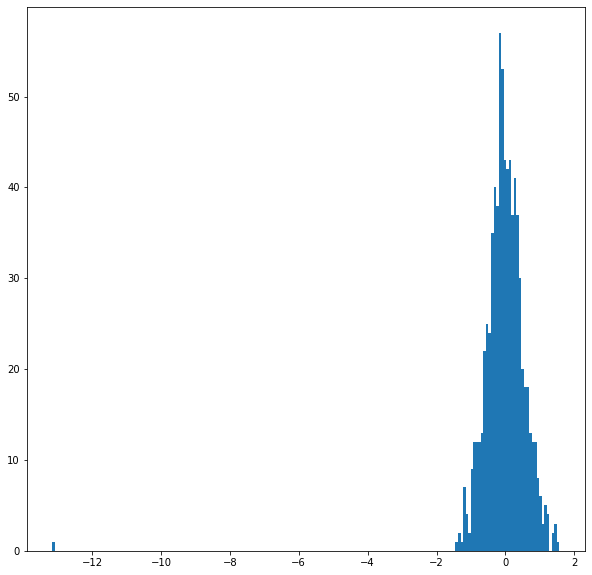
Let’s take a quick look at the range of values for a given layer and token.
You’ll find that the range is fairly similar for all layers and tokens, with the majority of values falling between [-2, 2], and a small smattering of values around -10.
# For the 5th token in our sentence, select its feature values from layer 5.
token_i = 5
layer_i = 5
vec = hidden_states[layer_i][batch_i][token_i]

# Plot the values as a histogram to show their distribution.
plt.figure(figsize=(10,10))
plt.hist(vec, bins=200)
plt.show()
Grouping the values by layer makes sense for the model, but for our purposes we want it grouped by token.
Current dimensions:
[# layers, # batches, # tokens, # features]
Desired dimensions:
[# tokens, # layers, # features]
Luckily, PyTorch includes the permute function for easily rearranging the dimensions of a tensor.
However, the first dimension is currently a Python list!
# `hidden_states` is a Python list.
print('      Type of hidden_states: ', type(hidden_states))

# Each layer in the list is a torch tensor.
print('Tensor shape for each layer: ', hidden_states[0].size())
      Type of hidden_states:  <class 'tuple'>
Tensor shape for each layer:  torch.Size([1, 22, 768])
Let’s combine the layers to make this one whole big tensor.
# Concatenate the tensors for all layers. We use `stack` here to
# create a new dimension in the tensor.
token_embeddings = torch.stack(hidden_states, dim=0)

token_embeddings.size()
torch.Size([13, 1, 22, 768])
Let’s get rid of the “batches” dimension since we don’t need it.
# Remove dimension 1, the "batches".
token_embeddings = torch.squeeze(token_embeddings, dim=1)

token_embeddings.size()
torch.Size([13, 22, 768])
Finally, we can switch around the “layers” and “tokens” dimensions with permute.
# Swap dimensions 0 and 1.
token_embeddings = token_embeddings.permute(1,0,2)

token_embeddings.size()
torch.Size([22, 13, 768])
Now, what do we do with these hidden states? We would like to get individual vectors for each of our tokens, or perhaps a single vector representation of the whole sentence, but for each token of our input we have 13 separate vectors each of length 768.
In order to get the individual vectors we will need to combine some of the layer vectors…but which layer or combination of layers provides the best representation?
Unfortunately, there’s no single easy answer… Let’s try a couple reasonable approaches, though. Afterwards, I’ll point you to some helpful resources which look into this question further.
Word Vectors
To give you some examples, let’s create word vectors two ways.
First, let’s concatenate the last four layers, giving us a single word vector per token. Each vector will have length 4 x 768 = 3,072.
# Stores the token vectors, with shape [22 x 3,072]
token_vecs_cat = []

# `token_embeddings` is a [22 x 12 x 768] tensor.

# For each token in the sentence...
for token in token_embeddings:

    # `token` is a [12 x 768] tensor

    # Concatenate the vectors (that is, append them together) from the last
    # four layers.
    # Each layer vector is 768 values, so `cat_vec` is length 3,072.
    cat_vec = torch.cat((token[-1], token[-2], token[-3], token[-4]), dim=0)

    # Use `cat_vec` to represent `token`.
    token_vecs_cat.append(cat_vec)

print ('Shape is: %d x %d' % (len(token_vecs_cat), len(token_vecs_cat[0])))
As an alternative method, let’s try creating the word vectors by summing together the last four layers.
# Stores the token vectors, with shape [22 x 768]
token_vecs_sum = []

# `token_embeddings` is a [22 x 12 x 768] tensor.

# For each token in the sentence...
for token in token_embeddings:

    # `token` is a [12 x 768] tensor

    # Sum the vectors from the last four layers.
    sum_vec = torch.sum(token[-4:], dim=0)

    # Use `sum_vec` to represent `token`.
    token_vecs_sum.append(sum_vec)

print ('Shape is: %d x %d' % (len(token_vecs_sum), len(token_vecs_sum[0])))
Sentence Vectors
To get a single vector for our entire sentence we have multiple application-dependent strategies, but a simple approach is to average the second to last hiden layer of each token producing a single 768 length vector.
# `hidden_states` has shape [13 x 1 x 22 x 768]

# `token_vecs` is a tensor with shape [22 x 768]
token_vecs = hidden_states[-2][0]

# Calculate the average of all 22 token vectors.
sentence_embedding = torch.mean(token_vecs, dim=0)
print ("Our final sentence embedding vector of shape:", sentence_embedding.size())
Our final sentence embedding vector of shape: torch.Size([768])
3.4. Confirming contextually dependent vectors
To confirm that the value of these vectors are in fact contextually dependent, let’s look at the different instances of the word “bank” in our example sentence:
“After stealing money from the bank vault, the bank robber was seen fishing on the Mississippi river bank.”
Let’s find the index of those three instances of the word “bank” in the example sentence.
for i, token_str in enumerate(tokenized_text):
  print (i, token_str)
0 [CLS]
1 after
2 stealing
3 money
4 from
5 the
6 bank
7 vault
8 ,
9 the
10 bank
11 robber
12 was
13 seen
14 fishing
15 on
16 the
17 mississippi
18 river
19 bank
20 .
21 [SEP]
They are at 6, 10, and 19.
For this analysis, we’ll use the word vectors that we created by summing the last four layers.
We can try printing out their vectors to compare them.
print('First 5 vector values for each instance of "bank".')
print('')
print("bank vault   ", str(token_vecs_sum[6][:5]))
print("bank robber  ", str(token_vecs_sum[10][:5]))
print("river bank   ", str(token_vecs_sum[19][:5]))
First 5 vector values for each instance of "bank".

bank vault    tensor([ 3.3596, -2.9805, -1.5421,  0.7065,  2.0031])
bank robber   tensor([ 2.7359, -2.5577, -1.3094,  0.6797,  1.6633])
river bank    tensor([ 1.5266, -0.8895, -0.5152, -0.9298,  2.8334])
We can see that the values differ, but let’s calculate the cosine similarity between the vectors to make a more precise comparison.
from scipy.spatial.distance import cosine

# Calculate the cosine similarity between the word bank
# in "bank robber" vs "river bank" (different meanings).
diff_bank = 1 - cosine(token_vecs_sum[10], token_vecs_sum[19])

# Calculate the cosine similarity between the word bank
# in "bank robber" vs "bank vault" (same meaning).
same_bank = 1 - cosine(token_vecs_sum[10], token_vecs_sum[6])

print('Vector similarity for  *similar*  meanings:  %.2f' % same_bank)
print('Vector similarity for *different* meanings:  %.2f' % diff_bank)
Vector similarity for  *similar*  meanings:  0.94
Vector similarity for *different* meanings:  0.69
This looks pretty good!
3.5. Pooling Strategy & Layer Choice
Below are a couple additional resources for exploring this topic.
BERT Authors
The BERT authors tested word-embedding strategies by feeding different vector combinations as input features to a BiLSTM used on a named entity recognition task and observing the resulting F1 scores.
(Image from Jay Allamar’s blog)
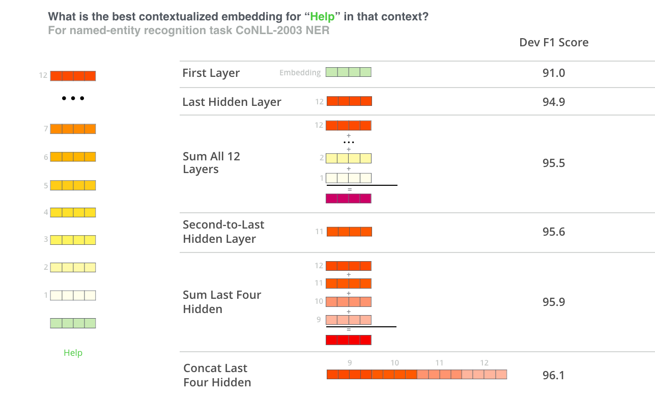
While concatenation of the last four layers produced the best results on this specific task, many of the other methods come in a close second and in general it is advisable to test different versions for your specific application: results may vary.
This is partially demonstrated by noting that the different layers of BERT encode very different kinds of information, so the appropriate pooling strategy will change depending on the application because different layers encode different kinds of information.
Han Xiao’s BERT-as-service
Han Xiao created an open-source project named bert-as-service on GitHub which is intended to create word embeddings for your text using BERT. Han experimented with different approaches to combining these embeddings, and shared some conclusions and rationale on the FAQ page of the project.
bert-as-service, by default, uses the outputs from the second-to-last layer of the model.
I would summarize Han’s perspective by the following:
- The embeddings start out in the first layer as having no contextual information (i.e., the meaning of the initial ‘bank’ embedding isn’t specific to river bank or financial bank).
- As the embeddings move deeper into the network, they pick up more and more contextual information with each layer.
- As you approach the final layer, however, you start picking up information that is specific to BERT’s pre-training tasks (the “Masked Language Model” (MLM) and “Next Sentence Prediction” (NSP)).
- What we want is embeddings that encode the word meaning well…
- BERT is motivated to do this, but it is also motivated to encode anything else that would help it determine what a missing word is (MLM), or whether the second sentence came after the first (NSP).
- The second-to-last layer is what Han settled on as a reasonable sweet-spot.
4. Appendix
4.1. Special tokens
It should be noted that although the [CLS] acts as an “aggregate representation” for classification tasks, this is not the best choice for a high quality sentence embedding vector. According to BERT author Jacob Devlin: “I’m not sure what these vectors are, since BERT does not generate meaningful sentence vectors. It seems that this is is doing average pooling over the word tokens to get a sentence vector, but we never suggested that this will generate meaningful sentence representations.”
(However, the [CLS] token does become meaningful if the model has been fine-tuned, where the last hidden layer of this token is used as the “sentence vector” for sequence classification.)
4.2. Out of vocabulary words
For out of vocabulary words that are composed of multiple sentence and character-level embeddings, there is a further issue of how best to recover this embedding. Averaging the embeddings is the most straightforward solution (one that is relied upon in similar embedding models with subword vocabularies like fasttext), but summation of subword embeddings and simply taking the last token embedding (remember that the vectors are context sensitive) are acceptable alternative strategies.
4.3. Similarity metrics
It is worth noting that word-level similarity comparisons are not appropriate with BERT embeddings because these embeddings are contextually dependent, meaning that the word vector changes depending on the sentence it appears in. This allows wonderful things like polysemy so that e.g. your representation encodes river “bank” and not a financial institution “bank”, but makes direct word-to-word similarity comparisons less valuable. However, for sentence embeddings similarity comparison is still valid such that one can query, for example, a single sentence against a dataset of other sentences in order to find the most similar. Depending on the similarity metric used, the resulting similarity values will be less informative than the relative ranking of similarity outputs since many similarity metrics make assumptions about the vector space (equally-weighted dimensions, for example) that do not hold for our 768-dimensional vector space.
4.4. Implementations
You can use the code in this notebook as the foundation of your own application to extract BERT features from text. However, official tensorflow and well-regarded pytorch implementations already exist that do this for you. Additionally, bert-as-a-service is an excellent tool designed specifically for running this task with high performance, and is the one I would recommend for production applications. The author has taken great care in the tool’s implementation and provides excellent documentation (some of which was used to help create this tutorial) to help users understand the more nuanced details the user faces, like resource management and pooling strategy.
Cite
Chris McCormick and Nick Ryan. (2019, May 14). BERT Word Embeddings Tutorial. Retrieved from http://www.mccormickml.com
BERT is an open source machine learning framework for natural language processing (NLP). BERT is designed to help computers understand the meaning of ambiguous language in text by using surrounding text to establish context. The BERT framework was pre-trained using text from Wikipedia and can be fine-tuned with question and answer datasets.
BERT, which stands for Bidirectional Encoder Representations from Transformers, is based on Transformers, a deep learning model in which every output element is connected to every input element, and the weightings between them are dynamically calculated based upon their connection. (In NLP, this process is called attention.)
Historically, language models could only read text input sequentially — either left-to-right or right-to-left — but couldn’t do both at the same time. BERT is different because it is designed to read in both directions at once. This capability, enabled by the introduction of Transformers, is known as bidirectionality.
Using this bidirectional capability, BERT is pre-trained on two different, but related, NLP tasks: Masked Language Modeling and Next Sentence Prediction.
The objective of Masked Language Model (MLM) training is to hide a word in a sentence and then have the program predict what word has been hidden (masked) based on the hidden word’s context. The objective of Next Sentence Prediction training is to have the program predict whether two given sentences have a logical, sequential connection or whether their relationship is simply random.
Background
Transformers were first introduced by Google in 2017. At the time of their introduction, language models primarily used recurrent neural networks (RNN) and convolutional neural networks (CNN) to handle NLP tasks.
Although these models are competent, the Transformer is considered a significant improvement because it doesn’t require sequences of data to be processed in any fixed order, whereas RNNs and CNNs do. Because Transformers can process data in any order, they enable training on larger amounts of data than ever was possible before their existence. This, in turn, facilitated the creation of pre-trained models like BERT, which was trained on massive amounts of language data prior to its release.
In 2018, Google introduced and open-sourced BERT. In its research stages, the framework achieved groundbreaking results in 11 natural language understanding tasks, including sentiment analysis, semantic role labeling, sentence classification and the disambiguation of polysemous words, or words with multiple meanings.
Completing these tasks distinguished BERT from previous language models such as word2vec and GloVe, which are limited when interpreting context and polysemous words. BERT effectively addresses ambiguity, which is the greatest challenge to natural language understanding according to research scientists in the field. It is capable of parsing language with a relatively human-like «common sense».
In October 2019, Google announced that they would begin applying BERT to their United States based production search algorithms.
BERT is expected to affect 10% of Google search queries. Organizations are recommended not to try and optimize content for BERT, as BERT aims to provide a natural-feeling search experience. Users are advised to keep queries and content focused on the natural subject matter and natural user experience.
In December 2019, BERT was applied to more than 70 different languages.
How BERT works
The goal of any given NLP technique is to understand human language as it is spoken naturally. In BERT’s case, this typically means predicting a word in a blank. To do this, models typically need to train using a large repository of specialized, labeled training data. This necessitates laborious manual data labeling by teams of linguists.
BERT, however, was pre-trained using only an unlabeled, plain text corpus (namely the entirety of the English Wikipedia, and the Brown Corpus). It continues to learn unsupervised from the unlabeled text and improve even as its being used in practical applications (ie Google search). Its pre-training serves as a base layer of «knowledge» to build from. From there, BERT can adapt to the ever-growing body of searchable content and queries and be fine-tuned to a user’s specifications. This process is known as transfer learning.
As mentioned above, BERT is made possible by Google’s research on Transformers. The transformer is the part of the model that gives BERT its increased capacity for understanding context and ambiguity in language. The transformer does this by processing any given word in relation to all other words in a sentence, rather than processing them one at a time. By looking at all surrounding words, the Transformer allows the BERT model to understand the full context of the word, and therefore better understand searcher intent.
This is contrasted against the traditional method of language processing, known as word embedding, in which previous models like GloVe and word2vec would map every single word to a vector, which represents only one dimension, a sliver, of that word’s meaning.
These word embedding models require large datasets of labeled data. While they are adept at many general NLP tasks, they fail at the context-heavy, predictive nature of question answering, because all words are in some sense fixed to a vector or meaning. BERT uses a method of masked language modeling to keep the word in focus from «seeing itself» — that is, having a fixed meaning independent of its context. BERT is then forced to identify the masked word based on context alone. In BERT words are defined by their surroundings, not by a pre-fixed identity. In the words of English linguist John Rupert Firth, «You shall know a word by the company it keeps.»
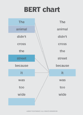
BERT is also the first NLP technique to rely solely on self-attention mechanism, which is made possible by the bidirectional Transformers at the center of BERT’s design. This is significant because often, a word may change meaning as a sentence develops. Each word added augments the overall meaning of the word being focused on by the NLP algorithm. The more words that are present in total in each sentence or phrase, the more ambiguous the word in focus becomes. BERT accounts for the augmented meaning by reading bidirectionally, accounting for the effect of all other words in a sentence on the focus word and eliminating the left-to-right momentum that biases words towards a certain meaning as a sentence progresses.
For example, in the image above, BERT is determining which prior word in the sentence the word «is» referring to, and then using its attention mechanism to weigh the options. The word with the highest calculated score is deemed the correct association (i.e., «is» refers to «animal», not «he»). If this phrase was a search query, the results would reflect this subtler, more precise understanding the BERT reached.
What is BERT used for?
BERT is currently being used at Google to optimize the interpretation of user search queries. BERT excels at several functions that make this possible, including:
- Sequence-to-sequence based language generation tasks such as:
- Question answering
- Abstract summarization
- Sentence prediction
- Conversational response generation
- Natural language understanding tasks such as:
- Polysemy and Coreference (words that sound or look the same but have different meanings) resolution
- Word sense disambiguation
- Natural language inference
- Sentiment classification
BERT is expected to have a large impact on voice search as well as text-based search, which has been error-prone with Google’s NLP techniques to date. BERT is also expected to drastically improve international SEO, because its proficiency in understanding context helps it interpret patterns that different languages share without having to understand the language completely. More broadly, BERT has the potential to drastically improve artificial intelligence systems across the board.
BERT is open source, meaning anyone can use it. Google claims that users can train a state-of-the-art question and answer system in just 30 minutes on a cloud tensor processing unit (TPU), and in a few hours using a graphic processing unit (GPU). Many other organizations, research groups and separate factions of Google are fine-tuning the BERT model architecture with supervised training to either optimize it for efficiency (modifying the learning rate, for example) or specialize it for certain tasks by pre-training it with certain contextual representations. Some examples include:
- patentBERT — a BERT model fine-tuned to perform patent classification.
- docBERT — a BERT model fine-tuned for document classification.
- bioBERT — a pre-trained biomedical language representation model for biomedical text mining.
- VideoBERT — a joint visual-linguistic model for process unsupervised learning of an abundance of unlabeled data on Youtube.
- SciBERT — a pretrained BERT model for scientific text
- G-BERT — a BERT model pretrained using medical codes with hierarchical representations using graph neural networks (GNN) and then fine-tuned for making medical recommendations.
- TinyBERT by Huawei — a smaller, «student» BERT that learns from the original «teacher» BERT, performing transformer distillation to improve efficiency. TinyBERT produced promising results in comparison to BERT-base while being 7.5 times smaller and 9.4 times faster at inference.
- DistilBERT by HuggingFace — a supposedly smaller, faster, cheaper version of BERT that is trained from BERT, and then certain architectural aspects are removed for the sake of efficiency.
This was last updated in January 2020
Continue Reading About BERT language model
- NLP uses in BI and analytics speak softly but carry a big stick
- Key considerations for operationalizing machine learning
- Wayfair takes a dip into NLP image processing technology
- AI for knowledge management boosts information accessibility
- BERT practical guide
Dig Deeper on AI technologies
-

large language model (LLM)
By: Sean Kerner
-
How to detect AI-generated content
By: Ron Karjian
-
lemmatization
By: Alexander Gillis
-
Exploring GPT-3 architecture
By: George Lawton


Trusted answers to developer questions
![]() Dian Us Suqlain
Dian Us Suqlain
Free System Design Interview Course
Many candidates are rejected or down-leveled due to poor performance in their System Design Interview. Stand out in System Design Interviews and get hired in 2023 with this popular free course.
As we all know, technological advancements and new trends are introduced daily. In 2018, Google published a paper on BERTBidirectional Encoder Representations from Transformers that totally changed Machine Learning practices and bridged a major gap.
Every word in BERT has its own importance and plays a vital role in Natural Language Processing.
Traditional models vs. BERT
Unlike other models that have previously worked unidirectionallyeither left-to-right or vice versa, BERT reads the entire sequence of sentences bidirectionallyin both directions. This is the reason for its effective and accurate results.
BERT understands the context in which the sentence is spoken
Take a look at the example above, previously, trained models couldn’t actually figure out the main context of the sentence. So, a model would have struggled with the word bank since it has two meaningsthe river bank and the bank where we handle financial matters.
BERT, on the other hand, checks both sides of the highlighted word and then generates its results accordingly. This is where the concept of transformers plays a major role.
Usage of BERT
There are multiple usages for Bert like:
- Hate speech analysis
- Text classification (Sentiment Analysis)
- Sentence Prediction
- Model training etc.
Most developers use BERT as it is pretrained on a significantly large corpus of unlabelled text including the entire Wikipedia — which alone includes 2,500 million words, and Book Corpus of 800 million words).
Architecture
There are currently two variants of BERT that are built on top of a transformer:
- 12 layers — BERT base
- 24 layers — BERT large
12 layers and 24 layers transformer blocks (BERT)
Sentiment analysis using BERT
To classify any statement, whether politically or in positive or negative remarks, every model has to understand the nature of the words spoken in it.
The BERT framework uses pre-training and fine-tuning to create tasks that include question answering systems, sentiment analysis, and language inference.
Fine-tuning and sentiment analysis
Sentence prediction with Bert
The primary objective of any NLP technique is to study human language and learn how it is spoken.
The simplest example for actual understanding of BERT can be Google searchWhenever you type something on the Google search bar, it automatically predicts the next sentence and shows a few suggestions in the dropdown.

Google search and Bert prediction
For detailed understanding
You can learn more about BERT and its implementation from the official Google blog.
CONTRIBUTOR
![]() Dian Us Suqlain
Dian Us Suqlain
Copyright ©2023 Educative, Inc. All rights reserved
Trusted Answers to Developer Questions
Learn in-demand tech skills in half the time
Copyright ©2023 Educative, Inc. All rights reserved.

Did you find this helpful?
BERT
What is BERT?
BERT, short for Bidirectional Encoder Representations from Transformers, is a machine learning (ML) framework for natural language processing. In 2018, Google developed this algorithm to improve contextual understanding of unlabeled text across a broad range of tasks by learning to predict text that might come before and after (bi-directional) other text.
Examples of BERT
BERT is used for a wide variety of language tasks. Below are examples of what the framework can help you do:
- Determine if a movie’s reviews are positive or negative
- Help chatbots answer questions
- Help predicts text when writing an email
- Can quickly summarize long legal contracts
- Differentiate words that have multiple meanings based on the surrounding text
Why is BERT important?
BERT converts words into numbers. This process is important because machine learning models use numbers, not words, as inputs. This allows you to train machine learning models on your textual data. That is, BERT models are used to transform your text data to then be used with other types of data for making predictions in a ML model.
BERT FAQs
Can BERT be used for topic modeling?
Yes. BERTopic is a topic modeling technique that uses BERT embeddings and a class-based TF-IDF to create dense clusters, allowing for easily interpretable topics while keeping important words in the topic descriptions.
What is Google BERT used for?
It’s important to note that BERT is an algorithm that can be used in many applications other than Google. When we talk about Google BERT, we are referencing its application in the search engine system. With Google, BERT is used to understand the intentions of the users’ search and the contents that are indexed by the search engine.
Is BERT a neural network?
Yes. BERT is a neural-network-based technique for language processing pre-training. It can be used to help discern the context of words in search queries.
Is BERT supervised or unsupervised?
BERT is a deep bidirectional, unsupervised language representation, pre-trained using a plain text corpus.
H2O.ai and BERT: BERT pre-trained models deliver state-of-the-art results in natural language processing (NLP). Unlike directional models that read text sequentially, BERT models look at the surrounding words to understand the context. The models are pre-trained on massive volumes of text to learn relationships, giving them an edge over other techniques. With GPU acceleration in H2O Driverless AI, using state-of-the-art techniques has never been faster or easier.
Bert vs Other Technologies & Methodologies
BERT vs GPT
Along with GPT (Generative Pre-trained Transformer), BERT receives credit as one of the earliest pre-trained algorithms to perform Natural Language Processing (NLP) tasks.
Below is a table to help you better understand the general differences between BERT and GPT.
| BERT | GPT |
|---|---|
| Bidirectional. Can process text left-to-right and right-to-left. BERT uses the encoder segment of a transformation model. | Autoregressive and unidirectional. Text is processed in one direction. GPT uses the decoder segment of a transformation model. |
| Applied in Google Docs, Gmail, smart compose, enhanced search, voice assistance, analyzing customer reviews, and so on. | Applied in application building, generating ML code, websites, writing articles, podcasts, creating legal documents, and so on. |
| GLUE score = 80.4% and 93.3% accuracy on the SQUAD dataset. | 64.3% accuracy on the TriviaAQ benchmark and 76.2% accuracy on LAMBADA, with zero-shot learning |
| Uses two unsupervised tasks, masked language modeling, fill in the blanks and next sentence prediction e.g. does sentence B come after sentence A? | Straightforward text generation using autoregressive language modeling. |
BERT vs transformer
BERT uses an encoder that is very similar to the original encoder of the transformer, this means we can say that BERT is a transformer-based model.
BERT vs word2vec
Consider the two examples sentences
- “We went to the river bank.”
- “I need to go to the bank to make a deposit.”
Word2Vec generates the same single vector for the word bank for both of the sentences. BERT will generate two different vectors for the word bank being used in two different contexts. One vector will be similar to words like money, cash, etc. The other vector would be similar to vectors like beach and coast.
BERT vs RoBERTa
Compared to RoBERTa (Robustly Optimized BERT Pretraining Approach), which was introduced and published after BERT, BERT is a significantly undertrained model and could be improved. RoBERTa uses a dynamic masking pattern instead of a static masking pattern. RoBERTa also replaces next sentence prediction objective with full sentences without NSP.
BERT Resources
BERT (англ. Bidirectional Encoder Representations from Transformers) — языковая модель, основанная на архитектуре трансформер, предназначенная для предобучения языковых представлений с целью их последующего применения в широком спектре задач обработки естественного языка.
Содержание
- 1 Модель и архитектура
- 1.1 Представление данных
- 2 Обучение
- 2.1 Предобучение
- 2.2 Точная настройка (Fine-tuning)
- 2.3 Гиперпараметры
- 2.4 Данные и оценка качества
- 3 Реализация
- 3.1 Пример использования
- 4 Возможности
- 4.1 Преимущества
- 4.2 Применение
- 5 См. также
- 6 Примечания
- 7 Источники информации
Модель и архитектура
BERT представляет собой нейронную сеть, основу которой составляет композиция кодировщиков трансформера. BERT является автокодировщиком.
В каждом слое кодировщика применяется двустороннее внимание, что позволяет модели учитывать контекст с обеих сторон от рассматриваемого токена, а значит, точнее определять значения токенов.
Представление данных
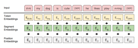
Рисунок 1. Представление входных данных модели
При подаче текста на вход сети сначала выполняется его токенизация. Токенами служат слова, доступные в словаре, или их составные части — если слово отсутствует в словаре, оно разбивается на части, которые в словаре присутствуют (см. рис. 1).
Словарь является составляющей модели — так, в BERT-Base[1] используется словарь около 30,000 слов.
В самой нейронной сети токены кодируются своими векторными представлениями (англ. embeddings), а именно, соединяются представления самого токена (предобученные), номера его предложения, а также позиции токена внутри своего предложения. Входные данные поступают на вход и обрабатываются сетью параллельно, а не последовательно, но информация о взаимном расположении слов в исходном предложении сохраняется, будучи включённой в позиционную часть эмбеддинга соответствующего токена.
Выходной слой основной сети имеет следующий вид: поле, отвечающее за ответ в задаче предсказания следующего предложения, а также токены в количестве, равном входному.
Обратное преобразование токенов в вероятностное распределение слов осуществляется полносвязным слоем с количеством нейронов, равным числу токенов в исходном словаре.
Обучение
Предобучение
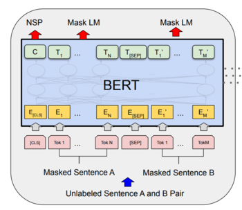
Рисунок 2. Схема этапа предобучения BERT
BERT обучается одновременно на двух задачах — предсказания следующего предложения (англ. next sentence prediction) и генерации пропущенного токена (англ. masked language modeling). На вход BERT подаются токенизированные пары предложений, в которых некоторые токены скрыты (см. рис. 2). Таким образом, благодаря маскированию токенов, сеть обучается глубокому двунаправленному представлению языка, учится понимать контекст предложения. Задача же предсказания следующего предложения есть задача бинарной классификации — является ли второе предложение продолжением первого. Благодаря ей сеть можно обучить различать наличие связи между предложениями в тексте.
Интерпретация этапа предобучения — обучение модели языку.
Точная настройка (Fine-tuning)
Этот этап обучения зависит от задачи, и выход сети, полученной на этапе предобучения, может использоваться как вход для решаемой задачи. Так, например, если решаем задачу построения вопросно-ответной системы, можем использовать в качестве ответа последовательность токенов, следующую за разделителем предложений. В общем случае дообучаем модель на данных, специфичных задаче: знание языка уже получено на этапе предобучения, необходима лишь коррекция сети.
Интерпретация этапа fine-tuning — обучение решению конкретной задачи при уже имеющейся общей модели языка.
Гиперпараметры
Гиперпараметрами модели являются — размерность скрытого пространства кодировщика, — количество слоёв-кодировщиков, — количество голов[2] в механизме внимания.
Данные и оценка качества
Предобучение ведётся на текстовых данных корпуса BooksCorpus[3] (800 млн. слов), а также на текстах англоязычной Википедии (2.5 млрд. слов).
Качество модели авторы оценивают на популярном для обучения моделей обработки естественного языка наборе задач GLUE.[4]
Реализация
В репозитории Google Research доступны для загрузки и использования несколько вариантов обученной сети в формате контрольных точек обучения модели популярного фреймворка TensorFlow[5]. В таблице в репозитории приведено соответствие параметров и и моделей. Использование моделей с малыми значениями гиперпараметров на устройствах с меньшей вычислительной мощностью позволяет сохранять баланс между производительностью и потреблением ресурсов. Также представлены модели с различным типом скрытия токенов при обучении, доступны два варианта: скрытие слова целиком (англ. whole word masking) или скрытие составных частей слов (англ. WordPiece masking).
Также модель доступна для использования с помощью популярной библиотеки PyTorch.[6]
Пример использования
Приведём пример предказания пропущенного токена при помощи BERT в составе PyTorch. Скрытый токен — первое слово второго предложения.
# Загрузка токенизатора и входные данные
tokenizer = torch.hub.load('huggingface/pytorch-transformers', 'tokenizer', 'bert-base-cased')
text_1 = "Who was Jim Henson ?"
text_2 = "Jim Henson was a puppeteer"

# Токенизация ввода, также добавляются специальные токены начала и конца предложения.
indexed_tokens = tokenizer.encode(text_1, text_2, add_special_tokens=True)
segments_ids = [0, 0, 0, 0, 0, 0, 0, 0, 1, 1, 1, 1, 1, 1, 1, 1]

# Конвертирвание ввода в формат тензоров PyTorch
segments_tensors = torch.tensor([segments_ids])
tokens_tensor = torch.tensor([indexed_tokens])
encoded_layers, _ = model(tokens_tensor, token_type_ids=segments_tensors)

# Выбираем токен, который будет скрыт и позднее предсказан моделью
masked_index = 8
indexed_tokens[masked_index] = tokenizer.mask_token_id
tokens_tensor = torch.tensor([indexed_tokens])

# Загрузка модели
masked_lm_model = torch.hub.load('huggingface/pytorch-transformers', 'modelWithLMHead', 'bert-base-cased')
predictions = masked_lm_model(tokens_tensor, token_type_ids=segments_tensors)

# Предсказание скрытого токена
predicted_index = torch.argmax(predictions[0][0], dim=1)[masked_index].item()
predicted_token = tokenizer.convert_ids_to_tokens([predicted_index])[0]
assert predicted_token == 'Jim'
Возможности
Преимущества
В отличие от прежних классических языковых моделей, BERT обучает контексто-зависимые представления. Например, word2vec[7] генерирует единственный эмбеддинг для одного слова, даже если слово многозначное и его смысл зависит от контекста. Использование BERT же позволяет учитывать окружающий контекст предложения, и генерировать различные эмбеддинги в таких случаях.
Контексто-зависимые модели в основном позволялют учитывать лишь левый или правый контекст токена. BERT же учитывает двусторонний контекст, что помогает модели лучше понимать смысл многозначных слов.
Применение
В 2019 году компания Google объявила об использовании BERT для анализа англоязычных поисковых запросов.[8] В конце того же года также было начато использование модели в алгоритме поиска на других языках.[9]
См. также
- Векторное представление слов
- Обработка естественного языка
- Автокодировщик
Примечания
- ↑ Github — Google Research — BERT
- ↑ Multi-Head Attention: Collaborate Instead of Concatenate
- ↑ Aligning Books and Movies: Towards Story-like Visual Explanations by Watching Movies and Reading Books
- ↑ GLUE: A Multi-Task Benchmark and Analysis Platform for Natural Language Understanding
- ↑ TensorFlow
- ↑ PyTorch
- ↑ word2vec
- ↑ Google Blog — Understanding searches better than ever before
- ↑ Search Engine Journal — Google’s BERT Rolls Out Worldwide
Источники информации
- BERT: Pre-training of Deep Bidirectional Transformers for Language Understanding — Оригинальная статья
- BERT (language model) — статья в англоязычной Википедии