Begins with number excel

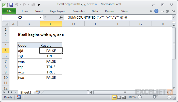
If cell begins with x, y, or z

Summary

To test values to see if they begin with one of several characters (i.e. begin with x, y, or z) , you can use the COUNTIF function together with the SUM function.

In the example shown, the formula in C5 is:

Generic formula

Explanation

The core of this formula is COUNTIF, which is configured to count three separate values using wildcards:

The asterisk (*) is a wildcard for one or more characters, so it is used to create a «begins with» test.

The values in the criteria are supplied in an «array constant», a hard-coded list of items with curly braces on either side.

When COUNTIF receives the criteria in an array constant, it will return multiple values, one per item in the list. Because we are only giving COUNTIF a one-cell range, it will only return two possible values for each criteria: 1 or 0.

In cell C5, COUNTIF evaluates to <0,0,0>. In cell C9, COUNTIF evaluates to: <0,1,0>. In each case, the first item is the result of criteria «x*», the second is from criteria «y*», and the third result is from criteria «z*».

Because we are testing for 3 criteria with OR logic, we only care if any result is not zero. To check this, we add up all items using the SUM function, and, to force a TRUE/FALSE result, we add «>0» to evaluate the result of SUM. In cell C5, we have:

Which evaluates to FALSE.

More criteria

The example shows 3 criteria (begins with x, y, or z) , but you add more criteria as needed.

Conditional formatting

Since this formula returns TRUE / FALSE, you can use it as-is to highlight values using conditional formatting.

Источник

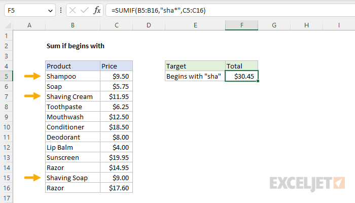
Sum if begins with

Summary

To sum numbers if values in a criteria range begin with specific text, you can use the SUMIF function or the SUMIFS function. In the example shown, the formula in F5 is:

The result is $30.45, the sum of Shampoo ($9.50), Shaving Cream (11.95), and Shaving Soap ($9.00). Note the SUMIF function is not case-sensitive.

Generic formula

Explanation

In this example, the goal is to sum the Price in column C when the Product in column B begins with «sha». To solve this problem, you can use either the SUMIF function or the SUMIFS function with the asterisk (*) wildcard, as explained below.

Wildcards

Certain Excel functions like SUMIF and SUMIFS support the wildcard characters «?» (any one character) and «*» (zero or more characters), which can be used in criteria. These wildcards allow you to create criteria such as «begins with», «ends with», «contains 3 characters», etc. as shown in the table below:

Target	Criteria
Cells with 3 characters	«. «
Cells like «bed», «bad», «bid», etc	«b?d»
Cells that begin with «xyz»	«xyz*»
Cells that end with «xyz»	«*xyz»

Note that wildcards are enclosed in double quotes («») when they appear in criteria.

SUMIF solution

The generic syntax for the SUMIF function looks like this:

In this example, the formula to sum Price when Product begins with «sha» is:

The criteria «sha*» means cells that begin with «sha». Notice you must enclose the text and the wildcard in double quotes («»). Also note that SUMIF is not case-sensitive. The criteria «sha*» will match «Shampoo», or «SHAMPOO».

SUMIFS solution

You can also use the SUMIFS function to sum if cells begin with. SUMIFS can handle multiple criteria, and the order of the arguments is different from SUMIF. The generic syntax for a single condition looks like this:

Notice that the sum range always comes first in the SUMIFS function. The equivalent SUMIFS formula for this example is:

The criteria used with SUMIFS is the same as that used in SUMIF, with the text and wildcard are both enclosed in double quotes («»). Like SUMIF, the SUMIFS function is not case-sensitive.

Источник

IF Function — Begins With

LinkBack

Thread Tools

Display

IF Function — Begins With

How do I apply the «begins with» filter to an IF statement? I would like to test a match on the first 3 characters of a string in a given cell?

This will look at the 3 leftmost characters and return a value if it is true.

Only indicate 3 characters in quotes. My last example had 4. Sorry!

Re: IF Function — Begins With

Would this formula work on numbers, or do I need to change the numbers to text first?

Re: IF Function — Begins With

What happened when you tried?

Re: IF Function — Begins With

Thanks! Long time lurker/learner from these forums, first time responding!

I got an answer, but it wasn’t the right one. It didn’t error out.
I think I’m going to try to do something along the line of the below since it is a number (once my brain can wrap around where this AND function goes along with the AND and ORs I already have going on. )

Re: IF Function — Begins With

Re: IF Function — Begins With

so I need to do something like if a3 starts with a then j3 has this output, or if a3 starts with x then j3has this output, I’m getting lost in the nesting

Re: IF Function — Begins With

Welcome to the forum.

We are happy to help, however whilst you feel your request is similar to this thread, experience has shown that things soon get confusing when answers refer to particular cells/ranges/sheets which are unique to your post and not relevant to the original.

Please see Forum Rule #4 about hijacking and start a new thread for your query.

If you are not familiar with how to start a new thread see the FAQ: How to start a new thread

1. Use code tags for VBA. [code] Your Code [/code] (or use the # button)
2. If your question is resolved, mark it SOLVED using the thread tools
3. Click on the star if you think someone helped you

Re: IF Function — Begins With

I am in need of an IF Function that will check the first three characters in Column B and Set a Text Value in Column A for that row

Example: If Cell B1 = P42ABC123N, Then cell A1 is set to «F32»

IF B1 Begins with P21, Set A1 to F21 or,
If B1 Begins with P24, Set A1 to F24 or,
If B1 Begins with P28, Set A1 to F28 or,
If B1 Begins with P12, Set A1 to F32 or,
If B1 Begins with P32, Set A1 to F32 or,
If B1 Begins with P42, Set A1 to F32 or,
If B1 Begins with P33, Set A1 to S33 or,
If B1 Begins with P46, Set A1 to S46

Re: IF Function — Begins With

Welcome to the forum.

We are happy to help, however whilst you feel your request is similar to this thread, experience has shown that things soon get confusing when answers refer to particular cells/ranges/sheets which are unique to your post and not relevant to the original.

Please see Forum Rule #4 about hijacking and start a new thread for your query.

If you are not familiar with how to start a new thread see the FAQ: How to start a new thread

Ali

Enthusiastic self-taught user of MS Excel who’s always learning!
Don’t forget to say «thank you» to anyone who has offered you help in your thread. You can reward them by clicking on * Add Reputation below theur user name on the left, if you wish.

Forum Rules (updated September 2018): please read them here.
How to use the Power Query code you’ve been given: help here. More about the Power suite here.

Источник

If number begins with excel

Подсчитайте числа, которые начинаются с определенного числа в Excel

Чтобы подсчитать количество ячеек, содержащих числа, начинающиеся с определенного числа в Excel, вы можете применить комбинацию функций СУММПРОИЗВ и ВЛЕВО.

Как подсчитать числа, начинающиеся с определенного числа в Excel?

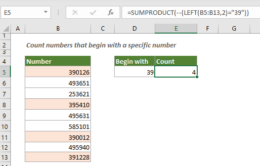
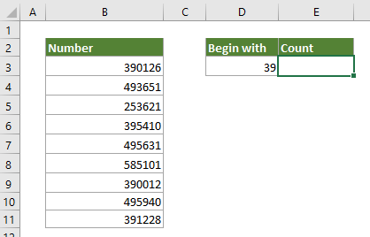
Как показано на скриншоте ниже, в столбце B есть список номеров, и вы хотите подсчитать общие числа, которые начинаются с числа «39». В этом случае следующая формула может оказать вам услугу.

Общая формула

=SUMPRODUCT(—(LEFT(range,n)=»number»))

аргументы

Как пользоваться этой формулой?

1. Выберите пустую ячейку, чтобы разместить результат.

2. Введите в нее приведенную ниже формулу и нажмите Enter ключ для получения результата.

=SUMPRODUCT(—(LEFT(B3:B11,2)=»39″))

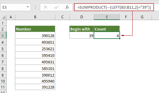
Примечание. В формуле B3: B11 — это диапазон столбцов, содержащий числа, которые вы будете подсчитывать, 39 — это заданное число, на основе которого вы будете считать числа, цифра 2 представляет количество символов, которые необходимо подсчитать. Вы можете изменить их по своему усмотрению.

Как работает эта формула?

=SUMPRODUCT(—(LEFT(B3:B11,2)=»39″))

• ЛЕВЫЙ (B3: B11,2): Функция LEFT извлекает первые две цифры из левой части чисел в диапазоне B3: B11 и возвращает массив, подобный этому: <«39»; «49»; «25»; «39»; «49»; «58 «;» 39 «;» 49 «;» 39 «>=» 39 «.
• <«39″;»49″;»25″;»39″;»49″;»58″;»39″;»49″;»39»>=»39″: Здесь сравнивайте каждое число в массиве с «39», если совпадение, возвращает ИСТИНА, в противном случае возвращает ЛОЖЬ. Вы получите массив как <ИСТИНА; ЛОЖЬ; ЛОЖЬ; ИСТИНА; ЛОЖЬ; ЛОЖЬ; ИСТИНА; ЛОЖЬ; ИСТИНА>.
• — (<ИСТИНА; ЛОЖЬ; ЛОЖЬ; ИСТИНА; ЛОЖЬ; ЛОЖЬ; ИСТИНА; ЛОЖЬ; ИСТИНА>): Эти два знака минус преобразуют «ИСТИНА» в 1 и «ЛОЖЬ» в 0. Здесь вы получите новый массив как <1; 0; 0; 1; 0; 0; 1; 0; 1>.
• =SUMPRODUCT : Функция СУММПРОИЗВ суммирует все числа в массиве и возвращает окончательный результат как 4.

Связанные функции

Функция СУММПРОИЗВ в Excel
Функцию СУММПРОИЗВ в Excel можно использовать для умножения двух или более столбцов или массивов, а затем получения суммы произведений.

Функция ВЛЕВО в Excel
Функция Excel LEFT извлекает заданное количество символов из левой части предоставленной строки.

Родственные формулы

Подсчет вхождений определенного текста во всей книге Excel
В этой статье будет продемонстрирована формула, основанная на функциях СУММПРОИЗВ, СЧЁТЕСЛИ и КОСВЕННО, для подсчета вхождений определенного текста во всей книге.

Подсчитайте несколько критериев с логикой НЕ в Excel
Эта статья покажет вам, как подсчитать количество ячеек с несколькими критериями с логикой НЕ в Excel.

Считайте или суммируйте только целые числа в Excel
В этом посте представлены две формулы на основе функции СУММПРОИЗВ и ИЗМЕНИТЬ, которые помогут вам подсчитывать и суммировать только целые числа в диапазоне ячеек в Excel.

Подсчитайте числа, где n-я цифра равна заданному числу
В этом руководстве представлена ​​формула, основанная на функциях СУММПРОИЗВ и СРЕДНЕЕ, для подсчета чисел, где n-я цифра равна заданному числу в Excel.

Kutools for Excel — поможет вам выделиться из толпы

Хотите быстро и качественно выполнять свою повседневную работу? Kutools for Excel предлагает мощные расширенные функции 300 (объединение книг, суммирование по цвету, разделение содержимого ячеек, преобразование даты и т. д.) и экономит для вас 80% времени.

• Разработан для 1500 рабочих сценариев, помогает решить 80% проблем с Excel.
• Уменьшите количество нажатий на клавиатуру и мышь каждый день, избавьтесь от усталости глаз и рук.
• Станьте экспертом по Excel за 3 минуты. Больше не нужно запоминать какие-либо болезненные формулы и коды VBA.
• 30-дневная неограниченная бесплатная пробная версия. 60-дневная гарантия возврата денег. Бесплатное обновление и поддержка 2 года.

Источник

How to count numbers that begin with specific value Excel

In this article, we will learn How to count numbers that begin with a given specific value Excel.

At instances when working with datasets. Sometimes we need to just get how many cells in the list which begins with a particular number. For Example finding the count of scores (above 10) in Exam where the student scored marks from 70 to 79 out of 100. For the above example you can use the double criteria one is number >= 70 & number

How to solve the problem?

For this, we will be using the SUMPRODUCT function and wildcard ( * ). SUMPRODUCT function counts the matched numbers. Here the criteria is the number must start with a particular given value. String can have any datatype like date, time, names or numbers. ( * ) character matches any number of uncertain characters in the string. LEFT function will extract the starting number from the string and match it with the given value in Excel.

= SUMPRODUCT (—( LEFT (range,n)=»num»)

range : list of values to match

num : given specific number

n : length of num value

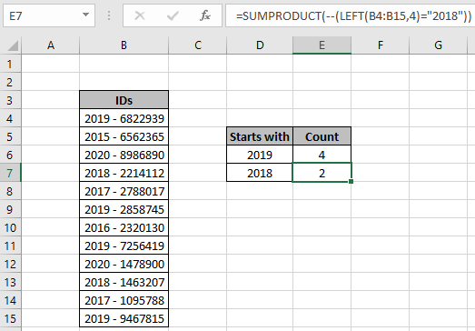
All of these might be confusing to understand. Let’s understand this formula using it in an example. Here we have a list of Ids having different year values attached as prefix. We need to find the count of IDs which start with 2019 year.

Use the formula:

= SUMPRODUCT (—( LEFT (B4:B15,4)=»2019″))

1. LEFT function extracts the first 4 characters from the list of IDs and matches it with the year value 2019.
2. The above process will create an array of TRUE and FALSE values. True value corresponding to the matched criteria.
3. SUMPRODUCT counts the number of TRUE values in the array and returns the count.

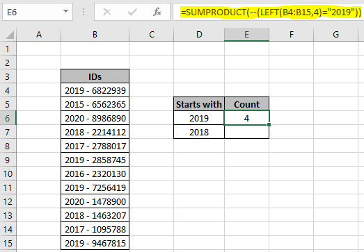
There are 4 Ids in the list (B4:B15) which lies in 2019. You can get the count of IDS having any year value from the Id list.

Now we can perform this function using the COUNTIF function. COUNTIF function returns the count of numbers using the asterisk wildcard. ( * ) wildcard matches any number of uncertain characters in length.

Use the formula:

= COUNTIF (B4:B15,»2018*»))

B3:B14 : range to match with

2018 : num value to start with

* : wildcard use to match any suffix with 2018.

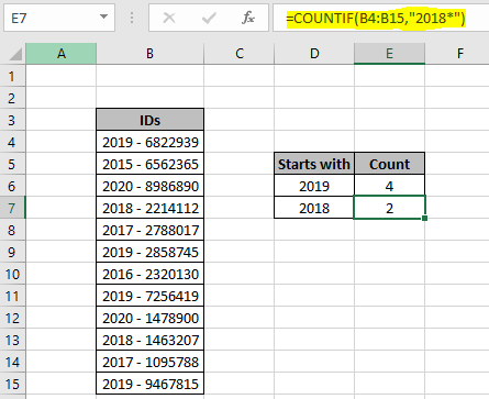
As you can see there are 2 Ids which do not lay in 2018. If you have more than one criteria to match then use the COUNTIFS function in Excel. You can also extract the count of numbers which ends with a given value using wildcard here.

Use the SUMPRODUCT function to count rows in the list. Learn more about Countif with SUMPRODUCT in Excel here .

Here are some observational notes shown below.

1. The formula works with numbers, text, date values, etc.
2. Use the same data type to match criteria in criteria list like name in names list, date in date values.
3. Lists as criteria ranges must be of same length, or the formula returns #VALUE! error.
4. Operators like equals to ( = ), less than equal to ( ), greater than ( > ) or not equals to ( <> ) can be used in criteria arguments, with numbers list only.
5. For example matching time values which have hour value 6. So you can use «06:*:*». Each ( * ) asterisk character is used for the uncertain minutes and seconds.

Hope this article about How to count numbers that begin with specific value Excel is explanatory. Find more articles on Counting values in the table using formulas here. If you liked our blogs, share it with your friends on Facebook . And also you can follow us on Twitter and Facebook . We would love to hear from you, do let us know how we can improve, complement or innovate our work and make it better for you. Write us at info@exceltip.com

How to use the COUNTIF Function in Excel : Count values with conditions using this amazing function. You don’t need to filter your data to count specific values. Countif function is essential to prepare your dashboard.

How to use the SUMPRODUCT function in Excel : Returns the SUM after multiplication of values in multiple arrays in excel.

COUNTIFS with Dynamic Criteria Range : Count cells selecting the criteria from the list of options in criteria cell in Excel using data validation tool.

COUNTIFS Two Criteria Match : multiple criteria match in different lists in table using the COUNTIFS function in Excel

COUNTIFS With OR For Multiple Criteria : match two or more names in the same list using the OR criteria applied on the list in Excel.

How to Use Countif in VBA in Microsoft Excel : Count cells with criteria using Visual Basic for Applications code in Excel macros.

How to use wildcards in excel : Count cells matching phrases in text lists using the wildcards ( * , ? ,

How to use the IF Function in Excel : The IF statement in Excel checks the condition and returns a specific value if the condition is TRUE or returns another specific value if FALSE.

How to use the VLOOKUP Function in Exceln : This is one of the most used and popular functions of excel that is used to lookup value from different ranges and sheets.

How to Use SUMIF Function in Excel : This is another dashboard essential function. This helps you sum up values on specific conditions.

The COUNTIFS Function in Excel : Learn more about COUNTIFS function in Excel here.

Источник

Предположим, есть список значений данных, которые начинаются с числовых цифр и за которыми следуют несколько букв или наоборот. И теперь вы хотите отфильтровать данные, которые начинаются с цифр или начинаются только с букв, как показано на следующих снимках экрана. Есть ли какие-нибудь хорошие приемы для решения этой задачи в Excel?

		Фильтр начинается с букв		Фильтр начинается с цифр

Отфильтровать данные, начинающиеся с буквы или цифры, с помощью вспомогательного столбца

---

Отфильтровать данные, начинающиеся с буквы или цифры, с помощью вспомогательного столбца

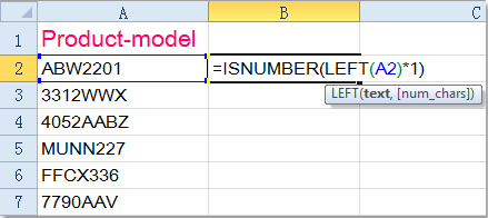
К сожалению, у вас нет прямой функции фильтрации данных, которые начинаются только с буквы или цифры. Но здесь вы можете создать вспомогательный столбец, чтобы справиться с этим.

1. Рядом со списком данных введите эту формулу: = ЕЧИСЛО (ЛЕВО (A2) * 1) (A2 указывает первые данные, исключая заголовок в вашем списке) в пустую ячейку, см. снимок экрана:

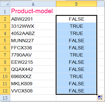
2. Затем перетащите маркер заполнения в диапазон, в котором вы хотите применить эту формулу, и все данные, начинающиеся с числа, будут отображаться как ИСТИНА, а остальные, начинающиеся с буквы, отображаются как НЕПРАВДА, см. снимок экрана:

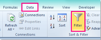
3. Затем отфильтруйте данные по этому новому столбцу, выберите ячейку B1 и щелкните Данные > Фильтр.

4. Затем щелкните рядом с ячейкой B1 и отметьте True или False, как вам нужно, см. снимок экрана:

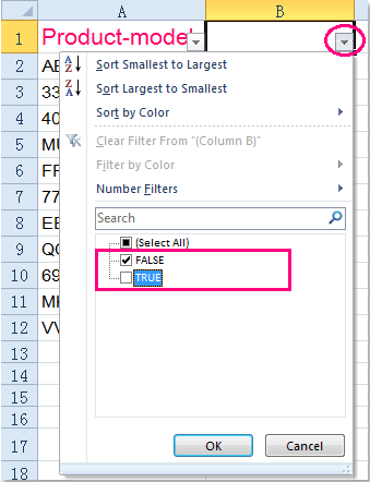
5. Затем нажмите OK, все необходимые данные были отфильтрованы. Если вы проверите Правда вариант, вы отфильтруете только данные, начинающиеся с числа, и если вы отметите Ложь вариант, вы отфильтруете все данные, которые начинаются с буквы. Смотрите скриншоты:

6. Наконец, вы можете удалить вспомогательный столбец, как хотите.

---

Статьи по теме:

Как фильтровать данные по кварталу в Excel?

Как фильтровать только целые или десятичные числа в Excel?

---

Лучшие инструменты для работы в офисе

Kutools for Excel Решит большинство ваших проблем и повысит вашу производительность на 80%

• Снова использовать: Быстро вставить сложные формулы, диаграммы и все, что вы использовали раньше; Зашифровать ячейки с паролем; Создать список рассылки и отправлять электронные письма …
• Бар Супер Формулы (легко редактировать несколько строк текста и формул); Макет для чтения (легко читать и редактировать большое количество ячеек); Вставить в отфильтрованный диапазон…
• Объединить ячейки / строки / столбцы без потери данных; Разделить содержимое ячеек; Объединить повторяющиеся строки / столбцы… Предотвращение дублирования ячеек; Сравнить диапазоны…
• Выберите Дубликат или Уникальный Ряды; Выбрать пустые строки (все ячейки пустые); Супер находка и нечеткая находка во многих рабочих тетрадях; Случайный выбор …
• Точная копия Несколько ячеек без изменения ссылки на формулу; Автоматическое создание ссылок на несколько листов; Вставить пули, Флажки и многое другое …
• Извлечь текст, Добавить текст, Удалить по позиции, Удалить пробел; Создание и печать промежуточных итогов по страницам; Преобразование содержимого ячеек в комментарии…
• Суперфильтр (сохранять и применять схемы фильтров к другим листам); Расширенная сортировка по месяцам / неделям / дням, периодичности и др .; Специальный фильтр жирным, курсивом …
• Комбинируйте книги и рабочие листы; Объединить таблицы на основе ключевых столбцов; Разделить данные на несколько листов; Пакетное преобразование xls, xlsx и PDF…
• Более 300 мощных функций. Поддерживает Office/Excel 2007-2021 и 365. Поддерживает все языки. Простое развертывание на вашем предприятии или в организации. Полнофункциональная 30-дневная бесплатная пробная версия. 60-дневная гарантия возврата денег.

---

Вкладка Office: интерфейс с вкладками в Office и упрощение работы

• Включение редактирования и чтения с вкладками в Word, Excel, PowerPoint, Издатель, доступ, Visio и проект.
• Открывайте и создавайте несколько документов на новых вкладках одного окна, а не в новых окнах.
• Повышает вашу продуктивность на 50% и сокращает количество щелчков мышью на сотни каждый день!

Комментарии (1)

Оценок пока нет. Оцените первым!

How to Filter a Column with Numbers Begins with or Starts with In Excel
Generally the Number Filters are look like as follows , where we do not have any option to Filter the Numbers starts with/begins with like «12***» or «21***» , as we have in Text Filters


Number Filters :

Text Filters :

In the above Text Filters , we have the Options like < Begins with > , < Ends with >.and we dont have any such options in Number Filters. 


But , still if we want to apply the Filter on a Numeric Column to Filter the Numbers starts with «12***» or «21***» , we have to do the following things :


First select the Numeric Column on which we want to apply the Filters.
Next , Change the data Format of Column and each Cell in Selection to Text using the below Code :


Selection.NumberFormat = «@»
For Each xCell In Selection
xCell.Value = CStr(xCell.Value)
Next xCell

Exit For
End If
Next X


Now the Numeric Column has been changed as Text based Column and we can see the Text Filters on that Column.

Example :
Suppose we have a Data follows int the < Master > Tab of a Workbook as follows :

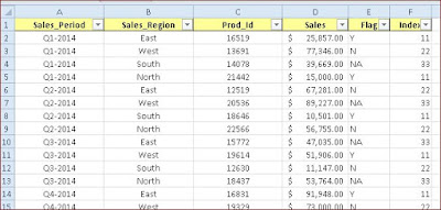
In the above data, we have a Numeric Field called < Prod_Id > , from this Field, we wish to Filter Numbers starts with «12*» or «21*» and then copy this Filtered Range to a New sheet < Filtered_Prod_Id > .
This can be done using the below Macro :


Sub Trans_Filtered_Acct()


Dim WS As Worksheet
Dim New_WS As Worksheet


Set WS = ThisWorkbook.Sheets(«Master»)
WS.Activate


For X = 1 To 20
‘Finding the <ACCT> Column Number Dynamically
If WS.Cells(1, X) = «Prod_Id» Then
C = Cells(1, X).Column
CN = Split(Cells(, c).Address, «$»)(1)


Set LastDataCell = WS.Cells.Find(«*», WS.Cells(1, 1), , , xlByRows, xlPrevious)
RC = LastDataCell.Row


‘Selecting the the <Prod_ID> Column
WS.Range(CN & «1:» & CN & RC).Select
Selection.NumberFormat = «@»


‘Converting the <Prod_ID> Column data to Text Format
For Each xCell In Selection
xCell.Value = CStr(xCell.Value)
Next xCell


Exit For
End If


Next X


‘Applying Filter on <Prod_ID> Column
WS.Range(CN & «1»).Select
Selection.AutoFilter Field:=3, Criteria1:=»=12*», Operator:=xlOr, Criteria2:=»=21*»


‘Copying the All columns data in Filtered Range
‘ActiveSheet.AutoFilter.Range.Copy


(or)


‘Copying the Specific columns data in Filtered Range
Set MyRange = WS.Range(«A1:D» & RC).SpecialCells(xlCellTypeVisible)
MyRange.Copy


‘Adding a New Sheet(Filtered_Prod_Id) and Copying the Filtered <Prod_ID> data to it.
Set New_WS = Sheets.Add(After:=Sheets(Sheets.Count))
New_WS.Name = «Filtered_Prod_Id»
ActiveSheet.Range(«A1»).Select
Selection.PasteSpecial Paste:=xlPasteValues, Operation:=xlNone, SkipBlanks _
        :=False, Transpose:=False
ActiveSheet.Range(«A1»).Select
Application.CutCopyMode = False


‘Coming back to <Prod_ID> tab and clearing the Filter
WS.Activate
WS.Range(«A1»).Select
Selection.AutoFilter
New_WS.Activate
Set WS = Nothing
Set New_WS = Nothing


MsgBox «Filtered <Prod_ID> Data has been Copied to a New Tab «, vbOKOnly, «Job Over»



End Sub


Output :

Thanks,TAMATAM

Count Number That Begin With Specific Number in Microsoft Excel

The main purpose of this formula is to count numbers in a range that begins with specific numbers. Here we will learn how to count numbers that begin with a certain number in Microsoft Excel. That implies, with the help of a formula based on the SUMPRODUCT and LEFT functions you can able to count numbers in a range that begins with specific numbers. So, with the help of this formula, you can able to count numbers that begin with a certain number.

General Formula to Count Number That Begin With Specific Number 

=SUMPRODUCT(—(LEFT(range,chars)=»xx»))

The Explanation for the Count Number That Begin With Specific Number

So we know that with the help of the given formula above you can able to count numbers in a range that begins with specific numbers. Here we will learn how to count numbers that begin with a certain number in Microsoft Excel. As we know that, the SUMPRODUCT  function is very versatile and efficient and works very well with the arrays. Here we are using the LEFT function inside the SUMPRODUCT function as shown in the above formula. So, with the help of this formula, you can able to count numbers in a range that begins with specific numbers.

Did this page help you?


|  

Yes you are correct, that is not possible in AutoFilter.
Here’s a way though if your data are numbers.

ActiveSheet.Range("$A$8:$AF$1194").AutoFilter Field:=12, Criteria1:=">=1500"

Or this if you specifically want those with 15 in it.

ActiveSheet.Range("$A$8:$AF$1194").AutoFilter Field:=12, Criteria1:=">=1500" _
    Operator:=xlAnd, Criteria2:="<1600"

Edit1: Answer to follow-up in comment

You can change all your data into Text by using Text To Columns under Data Tab.
Steps:

1. Select the entire column where you have your data in number format.
2. Then click on Text To Columns. Press Next on the 1st and 2nd dialogue box.
3. On the 3rd dialogue box, select Text instead of General.

Now, all your data are in the form of text.
You can then use below code to filter all that begins with 15.

ActiveSheet.Range("$A$8:$AF$1194").AutoFilter Field:=12, Criteria1:="15*"

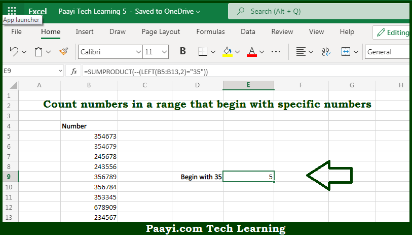
In this example, the goal is to count numbers in the range B5:B15 (named data) that begin with the numbers shown in column D. You would think this would be a good problem to solve with the COUNTIF function but for reasons explained below, COUNTIF won’t work. Instead, you can use the SUMPRODUCT and Boolean logic. See below for a full explanation.

COUNTIF function

The COUNTIF function returns the count of cells that meet one or more criteria, and supports logical operators (>,<,<>,=) and wildcards (*,?) for partial matching. You would think you could use the COUNTIF function with the asterisk wildcard (*) like this:

=COUNTIF(data,"25*") // returns 0

The problem however is using any wildcard character means criteria must be handled as a text value in double quotes («») whereas the values in column B are TRUE numbers. As a result, COUNTIF will never find a matching number and the result will always be zero. You might also think of this trick to coerce the numbers in data to text by concatenating an empty string («») to the range like this:

=COUNTIF(data&"","25*") // throws error

But this will throw an error, because COUNTIF is in a group of eight functions that require an actual range for range arguments. In other words, you can’t use an array operation in place of a range argument.

SUMPRODUCT function

Another way to solve this problem is with the SUMPRODUCT function, the LEFT function, and Boolean logic. To count numbers in data that begin with 25, we can use a formula like this:

=SUMPRODUCT(--(LEFT(data,2)="25")) // returns 5

Working from the inside out, the LEFT function is used to check all numbers in data like this:

LEFT(data,2)="25"

Because we give LEFT 11 numbers in the range B5:B15, LEFT returns an array with 11 results:

{"25";"25";"35";"45";"25";"45";"25";"45";"25";"35";"55"}="25"

We then compare each value to «25» to force a TRUE or FALSE result. Note that LEFT automatically converts the numbers to text, so we use the text value «25» for the comparison. The result is an array of TRUE and FALSE values:

{TRUE;TRUE;FALSE;FALSE;TRUE;FALSE;TRUE;FALSE;TRUE;FALSE;FALSE}

In this array, TRUE values correspond to numbers that begin with «25» and FALSE values represent numbers that don’t. We want to count these results, but first we need to convert the TRUE and FALSE values to 1s and 0s. To do this, we use a double negative (—).

--{TRUE;TRUE;FALSE;FALSE;TRUE;FALSE;TRUE;FALSE;TRUE;FALSE;FALSE}

The resulting array contains only 1s and 0s and is delivered directly to the SUMPRODUCT function:

=SUMPRODUCT({1;1;0;0;1;0;1;0;1;0;0})

With only a single array to process, SUMPRODUCT sums the items in the array and returns 5 as result. In this formula, note we are hardcoding the value «25» and the length of 2. To adapt the formula for the worksheet shown, where the numbers we want to count appear in column D, we use the LEN function and a reference to cell D5 like this:

=SUMPRODUCT(--(LEFT(data,LEN(D5))=D5))

The LEN function returns the number of characters in D5. This makes the formula more generic so it will support numbers of different lengths. Also note that the numbers in column D are entered as text values, since the result from LEFT will also be text. You can avoid this requirement by adapting the formula to coerce the value in D5 to text:

=SUMPRODUCT(--(LEFT(data,LEN(D5))=D5&""))

Here we concatenate an empty string («») to the D5, which converts any number to text. This version of the formula will work when there are numbers in column D, or text values.

Note: In Excel 365 and Excel 2021 you can use the SUM function instead of SUMPRODUCT if you prefer. This article provides more detail.

Extracting numbers from a list of cells with mixed text is a common data cleaning task.

Unfortunately, there is no direct menu or function created in Excel to help us accomplish this.

In this tutorial we will look at three cases where you might have a list of mixed text, from which you might want to extract numbers:

• When the number is always at the end of the text
• When the number is always at the beginning of the text
• When the number can be anywhere in the text

We will look at three different formulas that can be used to extract the numbers in each case.

At the end of the tutorial, we will also take a look at some VBA code that you can use to accomplish the same.

Brace yourself, this might get a little complex!

Extracting a Number from Mixed Text when Number is Always at the End of the Text

Consider the following example:

Here, each cell has a mix of text and numbers, with the number always appearing at the end of the text. In such cases, we will need to use a combination of nested Excel functions to extract the numbers.

The functions we will use are:

• FIND – This function searches for a character or string in another string and returns its position.
• MIN – This function returns the smallest value in a list.
• LEFT – This function extracts a given number of characters from the left side of a string.
• SUBSTITUTE – This function replaces a particular substring of a given text with another substring.
• IFERROR – This function returns an alternative result or formula if it finds an error in a given formula.

Essentially, we will be using the above functions altogether to perform the following sequence of tasks:

1. Find the position of the first numeric value in the given cell
2. Extract and remove the text part of the given cell (by removing everything to the left of the first numeric digit)

The formula that we will use to extract the numbers from cell A2 is as follows:

=SUBSTITUTE(A2,LEFT(A2,MIN(IFERROR(FIND({0,1,2,3,4,5,6,7,8,9},A2),""))-1),"")

Let us break down this formula to understand it better. We will go from the inner functions to the outer functions:

• FIND({0,1,2,3,4,5,6,7,8,9},A2) 

This function tries to find the positions of all the numbers (0-9) in the cell A2. Thus it returns an arrayformula:

{#VALUE!,#VALUE!,#VALUE!,#VALUE!,#VALUE!,#VALUE!,9,7,8,#VALUE!}

It returns a #VALUE! error for all digits except the 7th, 8th, and 9th digits because it was not able to find these numbers (0,1,2,3,4,5,9) in cell A2. It simply returns the positions of numbers 6,7 and 8 which are the 9th, 7th, and 8th characters respectively in A2.

• IFERROR(FIND({0,1,2,3,4,5,6,7,8,9},A2),””)

Next, the IFERROR function replaces all the error elements of the array with a blank (“”). As such it returns the arrayformula:

{“”,””,””,””,””,””,9,7,8,””}

• MIN(IFERROR(FIND({0,1,2,3,4,5,6,7,8,9},A2),””)) 

After this the MIN function finds the array element with least value. This is basically the position of the first numeric character in A2. The function now returns the value 7.

• LEFT(A2,MIN(IFERROR(FIND({0,1,2,3,4,5,6,7,8,9},A2),””))-1)

At this point we want to extract all text characters from A2 (so that we can remove them). So we want the LEFT function to extract all the characters starting backwards from the 7-1= 6th character. Thus we use the above formula. The result we get at this point is “arnold”. Notice we subtracted 1 from the second parameter of the LEFT function.

• SUBSTITUTE(A2,LEFT(A2,MIN(IFERROR(FIND({0,1,2,3,4,5,6,7,8,9},A2),””))-1),””)

Now all that’s left to do is remove the string obtained, by replacing it with a blank. This can be easily achieved by using the SUBSTITUTE function: We finally get the numeric characters in the mixed text, which is “786”.

Once you are done entering the formula, make sure you press CTRL+SHIFT+Enter, instead of just the return key. This is because the formula involves arrays.

In a nutshell, here’s what’s happening when you break down the formula:

=SUBSTITUTE(A2,LEFT(A2,MIN(IFERROR(FIND({0,1,2,3,4,5,6,7,8,9},A2),””))-1),””)

=SUBSTITUTE(A2,LEFT(A2,MIN(IFERROR({{#VALUE!,#VALUE!,#VALUE!,#VALUE!,#VALUE!,#VALUE!,9,7,8,#VALUE!}),””))-1),””)

=SUBSTITUTE(A2,LEFT(A2,MIN({“”,””,””,””,””,””,9,7,8,””}))-1),””)

=SUBSTITUTE(A2,”arnold”,””)

=786

When you drag the formula down to the rest of the cells, here’s the result you get:

Also read: How to Generate Random Letters in Excel?

Extracting a Number from Mixed Text when Number is Always at the Beginning of the Text

Now let us consider the case where the numbers are always at the beginning of the Text.

Consider the following example:

Here, each cell has a mix of text and numbers, with the number always appearing at the beginning of the text. In such cases, we will again need to use a combination of nested Excel functions to extract the numbers.

In addition to the functions we used in the previous formula, we are going to use two additional functions. These are:   

• MAX – This function returns the largest value in a list
• RIGHT – This function extracts a given number of characters from the right side of a string
• LEN – This function finds the length of (number of characters in) a given string.

Essentially, we will be using these functions altogether to perform the following sequence of tasks:

1. Find the position of the last numeric value in the given cell
2. Extract and remove the text part of the given cell (by removing everything to the right of the last numeric digit)

The formula that we will use to extract the numbers from cell A2 is as follows:

=SUBSTITUTE(A2,RIGHT(A2,LEN(A2)-MAX(IFERROR(FIND({0,1,2,3,4,5,6,7,8,9},A2),""))),"") 

Let us break down this formula to understand it better. We will go from the inner functions to the outer functions:

• FIND({0,1,2,3,4,5,6,7,8,9},A2) 

This function tries to find the positions of all the numbers (0-9) in the cell A2. Thus it returns an arrayformula:

{#VALUE!,#VALUE!,1,#VALUE!,#VALUE!,2,#VALUE!,#VALUE!,#VALUE!,#VALUE!}

It returns a #VALUE! error for all digits except the 3rd and 6th digits because it was not able to find these numbers (0,1,3,4,6,7,8,9) in cell A2. It simply returns the positions of numbers 2 and 5 which are the 1st and 2nd characters respectively in A2.

• IFERROR(FIND({0,1,2,3,4,5,6,7,8,9},A2),””)

Next, the IFERROR function replaces all the error elements of the array with a blank. As such it returns the array formula:

{“”,””,1,””,””,2,””,””,””,””}

• MAX(IFERROR(FIND({0,1,2,3,4,5,6,7,8,9},A2),””)) 

After this the MAX function finds the array element with the highest value. This is basically the position of the last numeric character in A2. The function now returns the value 2.

• LEN(A2)-MAX(IFERROR(FIND({0,1,2,3,4,5,6,7,8,9},A2),””))

At this point we want to extract all text characters from A2 (so that we can remove them). We need to specify how many characters we want to remove. This is obtained by computing the length of the string in A2 minus the position of the last numeric value.Thus we will get the value 8-2 = “6”.

• RIGHT(A2,LEN(A2)-MAX(IFERROR(FIND({0,1,2,3,4,5,6,7,8,9},A2),””)))

We can now use the RIGHT function to extract 6 characters starting from the 2nd character onwards. The result we get at this point is “arnold”.

• SUBSTITUTE(A2,RIGHT(A2,LEN(A2)-MAX(IFERROR(FIND({0,1,2,3,4,5,6,7,8,9},A2),””))),””)

Now all that’s left to do is remove this string by replacing it with a blank. This is easily achieved by using the SUBSTITUTE function. We finally get the numeric characters in the mixed text, which is “25”.

Again, once you are done entering the formula, don’t forget to press CTRL+SHIFT+Enter, instead of just the return key.

In a nutshell, here’s what’s happening when you break down the formula:

=SUBSTITUTE(A7,RIGHT(A7,LEN(A7)-MAX(IFERROR(FIND({0,1,2,3,4,5,6,7,8,9},A7),””))),””)

=SUBSTITUTE(A7,RIGHT(A7,LEN(A7)-MAX(IFERROR({#VALUE!,#VALUE!,1,#VALUE!,#VALUE!,2,#VALUE!,#VALUE!,#VALUE!,#VALUE!}

),””))),””)

=SUBSTITUTE(A7,RIGHT(A7,LEN(A7)-MAX({“”,””,1,””,””,2,””,””,””,””}

)),””)

=SUBSTITUTE(A7,RIGHT(A7,LEN(A7)-2),””)

=SUBSTITUTE(A7,RIGHT(A7,8-2),””)

=SUBSTITUTE(A7,”arnold”,””)

=25

When you drag the formula down to the rest of the cells, here’s the result you get:

Extracting a Number from Mixed Text when Number can be Anywhere in the Text

Finally let us consider the case where the numbers can be anywhere in the text, be it the beginning, end or middle part of the text.

Let’s take a look at the following example:

Here, each cell has a mix of text and numbers, where the number appears in any part of the text. In such cases, we will need to use a combination of nested Excel functions to extract the numbers.

Here are the functions that we are going to use this time:       

• INDIRECT – This function simply returns a reference to a range of values.
• ROW – This function returns a row number of a reference.
• MID – This function extracts a given number of characters from the middle of a string.
• TEXTJOIN – This function combines text from multiple ranges or strings using a specified delimiter between them.

Note that the formula discussed in this section will work only in Excel version 2016 onwards as it uses the newly introduced TEXTJOIN function. If you are using an older version of Excel, then you may consider using the VBA method instead (discussed in the next section).

In this method, we will essentially be using the above functions altogether to perform the following sequence of tasks:

1. Break up the given text into an array of individual characters
2. Find out and remove all characters that are not numbers
3. Combine the remaining characters into a full number

The formula that we will use to extract the numbers from cell A2 is as follows:

=TEXTJOIN("",TRUE,IFERROR(MID(A2,ROW(INDIRECT("1:"&LEN(A2))),1)*1,""))

Let us break down this formula to understand it better. We will go from the inner functions to the outer functions:

• LEN(A2) 

This function finds the length of the string in cell A2. In our case it returns 13.

• INDIRECT(“1:”&LEN(A2)) 

This function just returns a reference to all the rows from row 1 to row 12.

• ROW(INDIRECT(“1:”&LEN(A2))) 

Now this function returns the row numbers of each of these rows. In other words, it simply returns an array of numbers 1 to 12. This function thus returns the array:

{1;2;3;4;5;6;7;8;9;10;11;12;13}

Note: We use the ROW() function instead of simply hard-coding an array of numbers 1 to 12 because we want to be able to customize this formula depending on the size of the string being worked on. This will ensure that the function adjusts itself when copied to another cell. ·         

• MID(A2,ROW(INDIRECT(“1:”&LEN(A2))),1) 

Next the MID function extracts the character from A2 that corresponds to each position specified in the array. In other words, it returns an array containing each character of the text in A2 as a separate element, as follows:

{“a”;”r”;”n”;”o”;”l”;”d”;”1″;”4″;”3″;”b”;”l”;”u”;”e”}

• IFERROR(MID(A2,ROW(INDIRECT(“1:”&LEN(A2))),1)*1,””) 

After this, the IFERROR function replaces all the elements of the array that are non-numeric. This is because it checks if the array element can be multiplied by 1. If the element is a number, it can easily be multiplied to return the same number. But if the element is a non-numeric character, then it cannot be multiplied with 1 and thus returns an error. 

The IFERROR function here specifies that if an element gives an error on multiplication, the result returned will be blank. As such it returns the arrayformula:

{“”;””;””;””;””;””;1;4;3;””;””;””;””}

• TEXTJOIN(“”,TRUE,IFERROR(MID(A2,ROW(INDIRECT(“1:”&LEN(A2))),1)*1,””))

Finally, we can simply combine the array elements together using the TEXTJOIN function. The TEXTJOIN function here combines the string characters that remain (which are the numbers only) and ignores the empty string characters. We finally get the numeric characters in the mixed text, which is “143”.

Once you are done entering the formula, don’t forget to press CTRL+SHIFT+Enter, instead of just the return key.

In a nutshell, here’s what’s happening when you break down the formula:

=TEXTJOIN(“”,TRUE,IFERROR(MID(A2,ROW(INDIRECT(“1:”&LEN(A2))),1)*1,””))

=TEXTJOIN(“”,TRUE,IFERROR(MID(A2,ROW(INDIRECT(“1:”&13)),1)*1,””))

=TEXTJOIN(“”,TRUE,IFERROR(MID(A2,{1;2;3;4;5;6;7;8;9;10;11;12;13},1)*1,””))

=TEXTJOIN(“”,TRUE,IFERROR({“a”;”r”;”n”;”o”;”l”;”d”;”1″;”4″;”3″;”b”;”l”;”u”;”e”}

*1,””))

=TEXTJOIN(“”,TRUE,IFERROR(MID(A2,{1;2;3;4;5;6;7;8;9;10;11;12;13},1)*1,””))

=TEXTJOIN(“”,TRUE, {“”;””;””;””;””;””;1;4;3;””;””;””;””})

=143

When you drag the formula down to the rest of the cells, here’s the result you get:

Using VBA to Extract Number from Mixed Text in Excel

The above method works well enough in extracting numbers from anywhere in a mixed text.

However, it requires one to use the TEXTJOIN function, which is not available in older Excel versions (versions before Excel 2016).

If you’re on a version of Excel that does not support TEXTJOIN, then you can, instead, use a snippet of VBA code to get the job done.

If you have never used VBA before, don’t worry. All you need to do is copy the code below into your VBA developer window and run it on your worksheet data.

Here’s the code that you will need to copy:

'Code by Steve Scott from spreadsheetplanet.com 
Function ExtractNumbers(CellRef As String)
Dim StringLength As Integer
StringLength = Len(CellRef)
For i = 1 To StringLength
   If (IsNumeric(Mid(CellRef, i, 1))) Then Result = Result & Mid(CellRef, i, 1)
Next i
ExtractNumbers = Result
End Function

The above code creates a user-defined function called ExtractNumbers() that you can use in your worksheet to extract numbers from mixed text in any cell.

To get to your VBA developer window, follow these steps:

1. From the Developer tab, select Visual Basic.

1. Once your VBA window opens, Click Insert->Module. That’s it, you can now start coding.

Type or copy-paste the above lines of code into the module window. Your code is now ready to run.

Now, whenever you want to extract numbers from a cell, simply type the name of the function, passing the cell reference as a parameter. So to extract numbers from a cell A2, you will simply need to type the function as follows in a cell:

=ExtractNumbers(A2)

Explanation of the Code

Now let us take some time to understand how this code works.

• In this code, we defined a function named ExtractNumbers, that takes the string in the cell we want to work on. We assigned the name CellRef to this string.

Function ExtractNumbers(CellRef As String)

• We created a variable named StringLength, that will hold the length of the string, CellRef.

Dim StringLength As Integer

StringLength = Len(CellRef)

• Next, we loop through each character in the string CellRef and find out if it is a number. We use the function Mid(CellRef, i, 1) to extract a character from the string at each iteration of the loop. We also use the IsNumeric() function to find out if the extracted character is a number. Each extracted numeric character is combined together into a string called Result.

For i = 1 To StringLength

         If (IsNumeric(Mid(CellRef, i, 1))) Then Result = Result & Mid(CellRef, i, 1)

Next i

• This Result is then returned by the function.

ExtractNumbers = Result

Note that since the workbook now has VBA code in it, you need to save it with .xls or .xlsm extension.

You can also choose to save this to your Personal Macro Workbook, if you think you will be needing to run this code a lot. This will allow you to run the code on any Excel workbook of yours.

Well, that was a lot!

In this tutorial, we showed you how to extract numbers from mixed text in excel.

We saw three cases where the numbers are situated in different parts of the text. We also showed you how to use VBA to get the task done quickly.

Other Excel articles you may also like:

• How to Extract URL from Hyperlinks in Excel (Using VBA Formula)
• How to Reverse a Text String in Excel (Using Formula & VBA)
• How to Add Text to the Beginning or End of all Cells in Excel
• How to Remove Text after a Specific Character in Excel (3 Easy Methods)
• How to Separate Address in Excel?
• How to Extract Text After Space Character in Excel?
• How to Find the Last Space in Text String in Excel?
• How to Remove Space before Text in Excel

This article describes the formula syntax and usage of the FIND and FINDB functions in Microsoft Excel.

Description

FIND and FINDB locate one text string within a second text string, and return the number of the starting position of the first text string from the first character of the second text string.

Important: 

• These functions may not be available in all languages.

• FIND is intended for use with languages that use the single-byte character set (SBCS), whereas FINDB is intended for use with languages that use the double-byte character set (DBCS). The default language setting on your computer affects the return value in the following way:

• FIND always counts each character, whether single-byte or double-byte, as 1, no matter what the default language setting is.

• FINDB counts each double-byte character as 2 when you have enabled the editing of a language that supports DBCS and then set it as the default language. Otherwise, FINDB counts each character as 1.

The languages that support DBCS include Japanese, Chinese (Simplified), Chinese (Traditional), and Korean.

Syntax

FIND(find_text, within_text, [start_num])

FINDB(find_text, within_text, [start_num])

The FIND and FINDB function syntax has the following arguments:

• Find_text    Required. The text you want to find.

• Within_text    Required. The text containing the text you want to find.

• Start_num    Optional. Specifies the character at which to start the search. The first character in within_text is character number 1. If you omit start_num, it is assumed to be 1.

Remarks

• FIND and FINDB are case sensitive and don’t allow wildcard characters. If you don’t want to do a case sensitive search or use wildcard characters, you can use SEARCH and SEARCHB.

• If find_text is «» (empty text), FIND matches the first character in the search string (that is, the character numbered start_num or 1).

• Find_text cannot contain any wildcard characters.

• If find_text does not appear in within_text, FIND and FINDB return the #VALUE! error value.

• If start_num is not greater than zero, FIND and FINDB return the #VALUE! error value.

• If start_num is greater than the length of within_text, FIND and FINDB return the #VALUE! error value.

• Use start_num to skip a specified number of characters. Using FIND as an example, suppose you are working with the text string «AYF0093.YoungMensApparel». To find the number of the first «Y» in the descriptive part of the text string, set start_num equal to 8 so that the serial-number portion of the text is not searched. FIND begins with character 8, finds find_text at the next character, and returns the number 9. FIND always returns the number of characters from the start of within_text, counting the characters you skip if start_num is greater than 1.

Examples

Copy the example data in the following table, and paste it in cell A1 of a new Excel worksheet. For formulas to show results, select them, press F2, and then press Enter. If you need to, you can adjust the column widths to see all the data.

Data
Miriam McGovern
Formula	Description	Result
=FIND(«M»,A2)	Position of the first «M» in cell A2	1
=FIND(«m»,A2)	Position of the first «M» in cell A2	6
=FIND(«M»,A2,3)	Position of the first «M» in cell A2, starting with the third character	8

Example 2

Data
Ceramic Insulators #124-TD45-87
Copper Coils #12-671-6772
Variable Resistors #116010
Formula	Description (Result)	Result
=MID(A2,1,FIND(» #»,A2,1)-1)	Extracts text from position 1 to the position of «#» in cell A2 (Ceramic Insulators)	Ceramic Insulators
=MID(A3,1,FIND(» #»,A3,1)-1)	Extracts text from position 1 to the position of «#» in cell A3 (Copper Coils)	Copper Coils
=MID(A4,1,FIND(» #»,A4,1)-1)	Extracts text from position 1 to the position of «#» in cell A4 (Variable Resistors)	Variable Resistors

EXPLANATION
This tutorial shows how to count cells that begin with a specific value using Excel formulas and VBA.
This tutorial provides two Excel method that can be applied to count cells that begin with a specific value by using an Excel COUNTIF function and the «*» criteria. The first method references to a cell for the specific value and in the second method the specific value is directly entered into the formula. The formulas count the cells from range (B8:B14) that start with letter «b».
This tutorial provides two VBA methods that can be applied to count cells that begin with a specific value. The first method references to a cell for the specific value and in the second method the specific value is directly entered into the VBA code.

FORMULA (with value referenced to a cell)
=COUNTIF(range, value&»*»)

FORMULA (with value directly entered into the formula)
=COUNTIF(range, «value*»)

ARGUMENTS
range: The range of cells you want to count from.
value: The value that the cell begins with.