
So, you have decided that time has come to become an Excel Master. Congratulations!
Before you start with Excel functions and tools, there are some basics that need to be covered first.
Let’s start our magical journey in Excel together! 🙂
A really quick intro to Excel
Excel is the world’s most popular spreadsheet software, developed by Microsoft.
Excel debuted on September 30, 1985, and since that day, kept evolving to meet the requirements of the spreadsheet community.
Most of the Excel versions require installation on your local computer. However, In recent years, Excel can be used online, via Excel Online!
And the best thing? Excel Online is absolutely free.
This website utilizes the technology of Excel Online to help you learn and practice Excel without the need have Excel installed on your computer. Thanks Microsoft! 🙂
So, let’s finish with the talking and start practicing!
Typing in Excel
Excel can be used for complex calculations, but you can always use it to type regular text, just like you’d do in Word or any other software.
All you have to do is select one of the cells and start typing…
You can start by typing your name, your favorite pet, your favorite movie and your lucky number 🙂
When you finish typing, hit the Enter key to exit the cell edit mode.
As you can see, you can type both text and numbers in Excel.
Did you notice that certain parts of the sheets changed after you typed your details? This was done using Excel formulas, which we will cover in the next tutorials 🙂
How does Excel work?
Let’s discuss some of the basic ideas in Excel:
- Excel Cell
- Excel Range
- Excel Worksheet
- Excel Workbook
1. Excel Cell
The Excel Cell is the smallest unit in Excel. The cell is used to store data.
In the previous example, we typed our names and favorite pets, movies and numbers in different Excel Cells.
Excel is comprised of rows and columns. The rows are represented as numbers, and the columns – as letters.
In order to reference a specific cell in Excel, we will type its column letter, followed by the row number.
So, A1 will be the first cell in your worksheet – It’s in the first column (A), and in the first row (1):

Ok, now let’s practice… Type your First Name in cell C3, and your Last Name in cell C4
2. Excel Range
The Excel Range is comprised of two or more adjacent cells. These cells can be in the same row, the same column, or even in multiple rows and columns!
Each range is represented by two cells – The top-left cell, and the bottom-right cell, separated with colons.
For example, Range A3:E7 consists of the following cells:

Now, it’s your time to play with Excel ranges!
3. Excel Worksheet
The Excel Worksheet is comprised of rows and columns.
The default Excel Worksheet contains 1,048,576 rows and 16,384 columns.
In the following example, we have 4 different worksheets:

Tip – We can quickly navigate between worksheets using the shortcut Ctrl+Page Up/Ctrl+Page Down. Click here for more useful Excel shortcuts!
4. Excel Workbook
The Excel file is also called Excel Workbook. It contains one or more worksheets.
The default Excel file type has an XLSX suffix.
Excel allows the user to use data from one worksheet in another worksheet in the same workbook. It also allows connecting between different workbooks.
Basic Calculations with Excel
OK, let’s start with the fun part!
We can perform calculations in Excel easily.
In order to start a calculation in a cell, we will type the = sign (equals), and then type our calculation.
These are the basic operators which can be used:
+ Add
– Substract
/ Divide
* (Asterisk) Multiply
^ Power
So, let’s say we want to find the result of 2+2:

Ok, now let’s practice!
Cell References
Okay, now that we know how to perform basic calculations, let’s learn how we can use cell references to make our calculations much quicker, and dynamic, as well!
If we type the = (equals) sign, followed by a reference to a cell (either by typing the cell name or clicking it), we can reference the data stored in that cell. We can also perform calculations using this way – Instead of manually typing the numbers, we can just reference the cells containing these numbers!
Let’s see how it works:

You can see in the example above that each time we change the data in the referenced cell – It is automatically reflected in the second cell!
Now, time to play with Excel:
Reusing cell references & using Partial and Absolute References
One of the advantages of using cell references in Excel is that we can reuse cell references in adjacent cells by copying the cell, or by dragging the cell to adjacent cells.
Let’s see how it works:

Sometimes, we would like that a certain reference will not move if we reuse the formula in other cells.
In such cases, we can use an Absolute Reference, by hitting the F4 button (or manually typing the $ signs before the column and/or row – not recommended) after typing the cell reference.
Let’s see this in action:

In certain cases, we might prefer using a Partial Reference rather than an Absolute Reference.
A Partial Reference allows us to keep the same reference only for a part of the cell – either the row or the column.
To use Partial Reference, just hit the F4 button until the deserved result is achieved.
Let’s see how we can do the entire Multiplication Table calculation, using only one formula!

Now you are all set to continue your Excel journey and learn how to use Excel functions and tools. Good luck! 🙂
In an article written in 2018, Robert Half, a company specializing in human resources and the financial industry, wrote that 63% of financial firms continue to use Excel in a primary capacity. Granted, that is not 100% and is actually considered to be a decline in usage! But considering the software is a spreadsheet software and not designed solely as financial industry software, 63% is still a significant portion of the industry and helps to illustrate how important Excel is.
Learning how to use Excel doesn’t have to be difficult. Taking it one step at a time will help you move from a novice to an expert (or at least closer to that point) – at your pace.
As a preview of what we are going to cover in this article, think worksheets, basic usable functions and formulas, and navigating a worksheet or workbook. Granted, we will not be covering every possible Excel function but we will cover enough that it gives you an idea of how to approach the others.
Basic Definitions
It really is helpful if we cover a few definitions. More than likely, you have heard these terms (or already know what they are). But we will cover them to be sure and be all set for the rest of the process in learning how to use Excel.
Workbooks vs. Worksheets
Excel documents are called Workbooks and when you first create an Excel document (the workbook), many (not all) Excel versions will automatically include three tabs, each with its own blank worksheet. If your version of Excel doesn’t do that, don’t worry, we will learn how to create them.
The Worksheets are the actual parts where you enter the data. If it is easier to think of it visually, think of the worksheets as those tabs. You can add tabs or delete tabs by right-clicking and choosing the delete option. Those worksheets are the actual spreadsheets with which we work and they are housed in the workbook file.
The Ribbon
The Ribbon spreads across the Excel application like a row of shortcuts, but shortcuts that are represented visually (with text descriptions). This is helpful when you want to do something in short order and especially when you need help determining what you want to do.
There is a different grouping of ribbon buttons depending on which section/group you choose from the top menu options (i.e. Home, Insert, Data, Review, etc.) and the visual options presented will relate to those groupings.
Excel Shortcuts
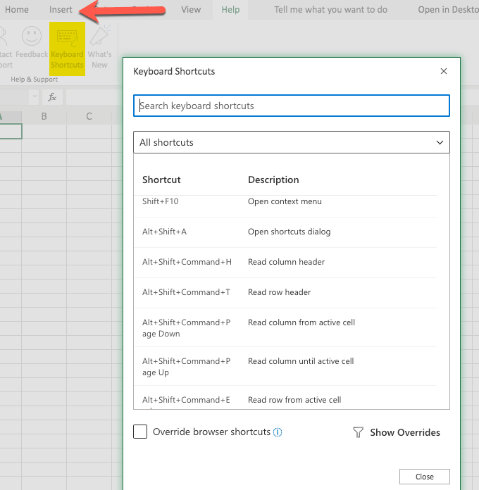
Shortcuts are helpful in navigating the Excel software quickly, so it is helpful (but not absolutely essential) to learn them. Some of them are learned by seeing the shortcuts listed in the menus of the older versions of the Excel application and then trying them out for yourself.
Another way to learn Excel shortcuts is to view a list of them on the website of the Excel developers. Even if your version of Excel doesn’t display the shortcuts, most of them still work.
Formulas vs. Functions
Functions are built-in capabilities of Excel and are used in formulas. For example, if you wanted to insert a formula that calculated the sum of numbers in different cells of a spreadsheet, you could use the function SUM() to do just that.
More on this function (and other functions) a bit further on in this article.
Formula Bar

The formula bar is an area that appears below the Ribbon. It is used for formulas and data. You enter the data in the cell and it will also appear in the formula bar if you have your mouse on that cell.
When we reference the formula bar, we are simply indicating that we should type the formula in that spot while having the appropriate cell selected (which, again, will automatically happen if you select the cell and start typing).
Creating & Formatting a Worksheet Example
There are many things you can do with your Excel Worksheet. We will give you some example steps as we go along in this article so you can try them out for yourself.
The First Workbook
It is helpful to start with a blank Workbook. So, go ahead and select New. This may vary, depending on your version of Excel, but is generally in the File area.
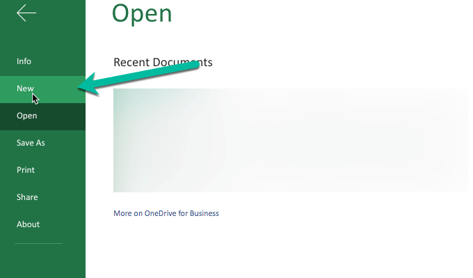
Note: The above image says Open at the top to illustrate that you can get to the New (left-hand side, pointed to with the green arrow) from anywhere. This is a screenshot of the newer Excel.
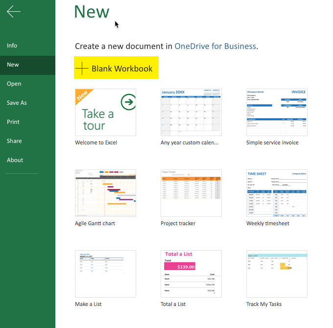
When you click on New you are more than likely going to get some example templates. The templates themselves may vary between versions of Excel, but you should get some sort of selection.
One way of learning how to use Excel is to play with those templates and see what makes them “tick”. For our article, we are starting with a blank document and playing around with data and formulas, etc.
So go ahead and select the blank document option. The interface will vary, from version to version, but should be similar enough to get the idea. A little later we will also download another sample Excel sheet.
Inserting the Data
There are many different ways to get data into your spreadsheet (a.k.a. worksheet). One way is to simply type what you want where you want it. Choose the particular cell and just start typing.
Another way is to copy data and then paste it into your Spreadsheet. Granted, if you are copying data that is not in a table format it can get a little interesting as to where it lands in your document. But fortunately we can always edit the document and recopy and paste elsewhere, as needed.
You can try the copy/paste method now by selecting a portion of this article, copying it, and then pasting into your blank spreadsheet.
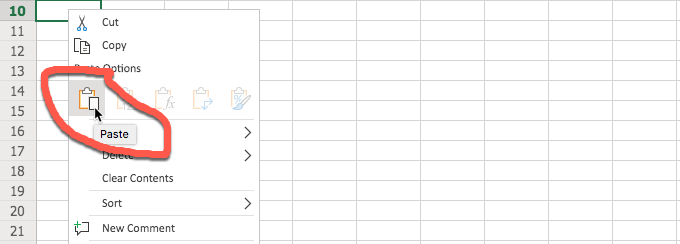
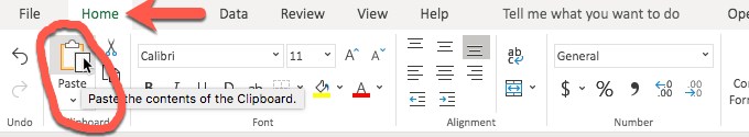
After selecting the portion of the article and copying it, go to your spreadsheet and click on the desired cell where you want to start the paste and do so. The method shown above is using the right-click menu and then selecting “Paste” in the form of the icon.
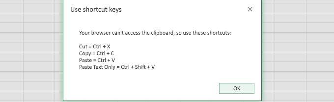
It is possible that you may get an error when using the Excel built-in paste method, even with the other Excel built-in methods as well. Fortunately, the error warning (above) helps to point you in the right direction to get the data you copied into the sheet.
When pasting the data, Excel does a pretty good job of interpreting it. In our example, I copied the first two paragraphs of this section and Excel presented it in two rows. Since there was an actual space between the paragraphs, Excel reproduced that as well (with a blank row). If you are copying a table, Excel does an even better job of reproducing it in the sheet.

Also, you can use the button in the Ribbon to paste. For visual people, this is really helpful. It is shown in the image below.
Some versions of Excel (especially the older versions) allow you to import data (which works best with similar files or CSV – comma-separated values – files). Some newer versions of Excel do not have that option but you can still open the other file (the one that you want to import), use a select all and then copy and paste it into your Excel spreadsheet.
When import is available, it is generally found under the File menu. In the new version(s) of Excel, you may be rerouted to more of a graphical user interface when you click on File. Simply click the arrow in the top left to return back to your worksheet.
Hyperlinking
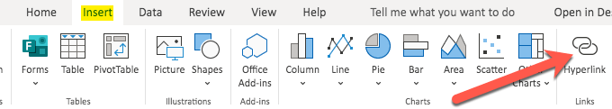
Hyperlinking is fairly easy, especially when using the Ribbon. You will find the hyperlink button under the Insert menu in the newer Excel versions. It may also be accessed via a shortcut like command-K.
Formatting Data (Example: Numbers and Dates)
Sometimes it is helpful to format the data. This is especially true with numbers. Why? Sometimes numbers automatically fall into a general format (sort of default) which is more like a text format. But often, we want our numbers to behave as numbers.
The other example would be dates, which we may want to format to ensure that all of our dates appear consistent, like 20200101 or 01/01/20 or whatever format we choose for our date format.
You can access the option to format your data in a couple of different ways, shown in the below images.
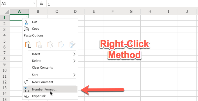
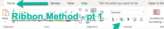
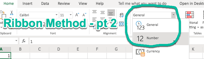
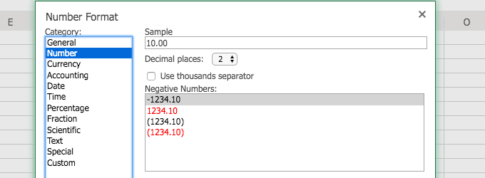
Once you have accessed, say, the Number format, you will have several options. These options appear when you use the right-click method. When you use the Ribbon, your options are right there in the Ribbon. It all depends on which is easier for you.
If you have been using Excel for a while, the right-click method, with the resulting number format dialog box (shown below) may be easier to understand. If you are newer or more visual, the Ribbon method may make more sense (and much quicker to use). Both provide you with number formatting options.
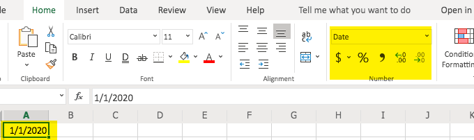
If you type anything that resembles a date, the newer versions of Excel are nice enough to reflect that in the Ribbon as shown in the below image.
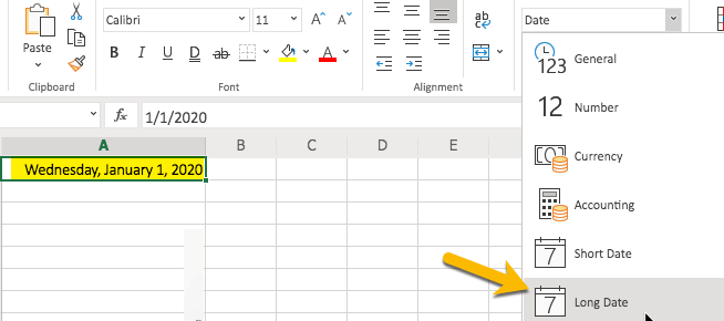
From the Ribbon you can select formats for your date. For example, you can choose a short date or a long date. Go ahead and try it and view your results.
Presentation Formatting (Example: Aligning Text)
It is also helpful to understand how to align your data, whether you want it all to line up to the left or to the right (or justified, etc). This too can be accessed via the Ribbon.
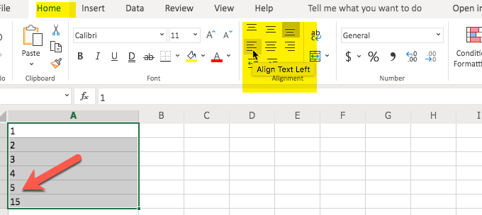
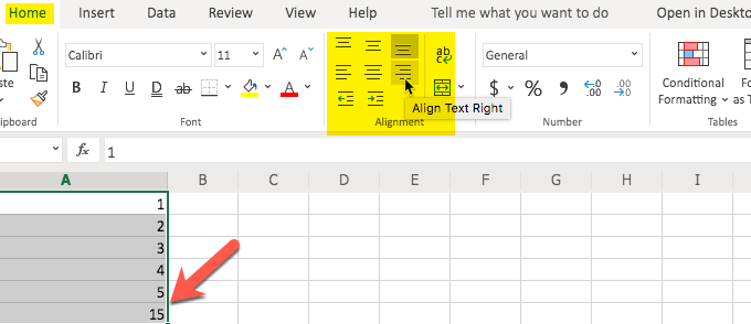
As you can see from the images above, the alignment of the text (i.e. right, left, etc.) is on the second row of the Ribbon option. You can also choose other alignment options (i.e. top, bottom) in the Ribbon.
Also, if you notice, aligning things like numbers may not look right when aligned left (where text looks better) but does look better when aligned right. The alignment is very similar to what you would see in a word processing application.
Columns & Rows
It is helpful to know how to work with, as well as adjust the width and dimensions of, columns and rows. Fortunately, once you get the hang of it, it is fairly easy to do.
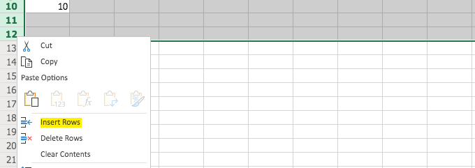
There are two parts to adding or deleting rows or columns. The first part is the selection process and the other is the right-click and choosing the insert or delete option.
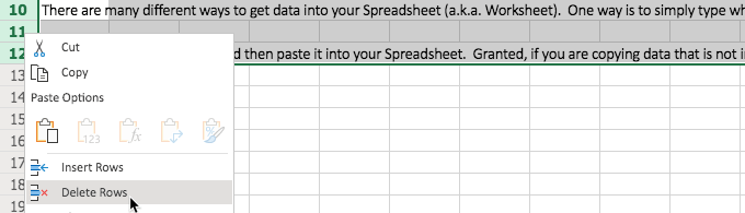
Remember the data we copied from this article and pasted into our blank Excel sheet in the above example? We probably don’t need it anymore so it is a perfect example for the process of deleting rows.
Remember our first step? We need to select the rows. Go ahead and click on the row number (to the left of the top left cell) and drag downward with your mouse to the bottom row that you want to delete. In this case, we are selecting three rows.
Then, the second part of our procedure is to click on Delete Rows and watch Excel delete those rows.

The process for inserting a row is similar but you do not have to select more than one row. Excel will determine where you click is where you want to insert the row.
To start the process, click on the row number that you want to be below the new row. This tells Excel to select the entire row for you. From the spot where you are, Excel will insert the row above that. You do so by right-clicking and choosing Insert Rows.
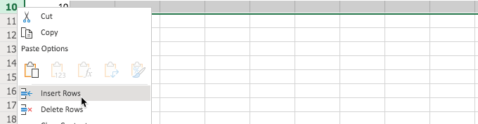
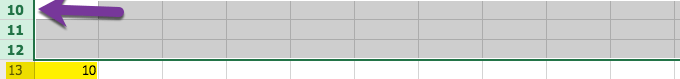
As you can see above, we typed 10 in row 10. Then, after selecting 10 (row 10), right-clicking, and choosing Insert Rows, the number 10 went down one row. It resulted in the 10 now being in row 11.
This demonstrates how the inserted row was placed above the selected row. Go ahead and try it for yourself, so you can see how the insertion process works.
If you need more than one row, you can do so by selecting more than one row and this tells Excel how many you want and that quantity will be inserted above the row number selected.
The following pictures show this in a visual format, including how the 10 went down three rows, the number of rows inserted.
Inserting and deleting columns is basically the same except that you are selecting from the top (columns) instead of the left (rows).
Filters & Duplicates
When we have a lot of data to work with it helps if we have a couple of tricks up our sleeves in order to more easily work with that data.
For example, let’s say you have a bunch of financial data but you only need to look at specific data. One way to do that is to use an Excel “Filter.”
First, let’s find an Excel Worksheet that presents a lot of data so we have something to test this on (without having to type all of the data ourselves). You can download just such a sample from Microsoft. Keep in mind that that is the direct link to the download so the Excel example file should start downloading right away when you click on that link.
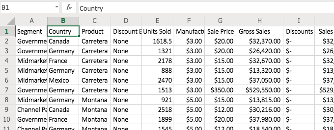
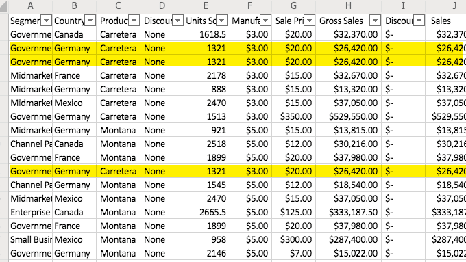
Now that we have the document, let’s look at the volume of data. Quite a bit, isn’t it? Note: the image above will look a bit different from what you have in your sample file and that is normal.
Let’s say you only wanted to see data from Germany. Use the “Filter” option in the Ribbon (under “Home”). It is combined with the “Sort” option towards the right (in the newer Excel versions).
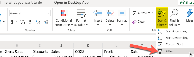
Now, tell Excel what options you want. In this case, we are looking for data on Germany as the selected country.
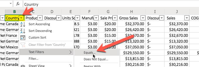
You will notice that when you select the filter option, little pull-down arrows appear in the columns. When an arrow is selected, you have several options, including the “Text Filters” option that we will be using. You have an option to sort ascending or descending.
It makes sense why Excel combines these in the Ribbon since all of these options appear in the pull-down list. We will be selecting the “Equals…” under the “Text Filters.”
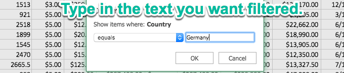
After we select what we want to do (in this case Filter), let’s provide the information/criteria. We would like to see all the data from Germany so that is what we type in the box. Then, click “OK.”
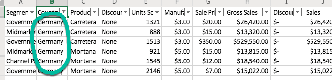
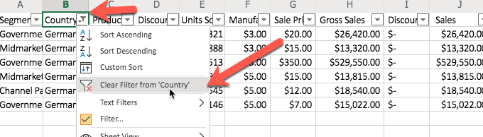
You will notice that now we only see data from Germany. The data has been filtered. The other data is still there. It is just hidden from view. There will come a time when you want to discontinue the filter and see all of the data. Simply return to the pull-down and choose to clear the filter, as shown in the below image.
Sometimes you will have data sets that include duplicate data. It is much easier if you only have singular data. For example, why would you want the exact same financial data record twice (or more) in your Excel Worksheet?
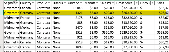
Below is an example of a data set that has some data that is repeated (shown highlighted in yellow).
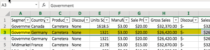
To remove duplicates (or more, as in this case), start by clicking on one of the rows that represents the duplicate data (that contains the data that is repeated). This is shown in the below image.
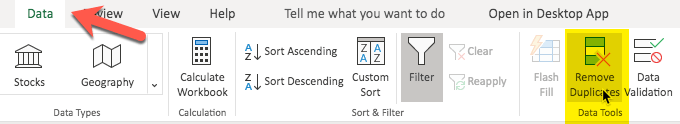
Now, visit the “Data” tab or section and from there, you can see a button on the Ribbon that says “Remove Duplicates.” Click that.
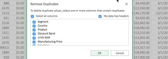
The first portion of this process presents you with a dialog box similar to what you see in the below image. Don’t let this confuse you. It is simply asking you which column to look at when identifying the duplicate data.
For example, if you had several rows with the same first and last name but basically gibberish in the other columns (like a copy/paste from a website for example) and you only needed unique rows for the first and last name, you would select those columns so that the gibberish that may not be duplicate does not come into consideration in removing the excess data.
In this case, we left the selection as “all columns” because we had duplicated rows manually so we knew that all of the columns were exactly the same in our example. (You can do the same with the Excel example file and test it.)
After you click “OK” on the above dialog box, you will see the result and in this case, three rows were identified as matching and two of them were removed.
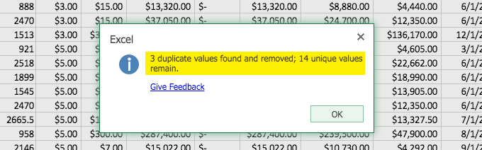
Now, the resulting data (shown below) matches the data we started with before we went through the addition and removal of duplicates.
You have just learned a couple tricks. These are especially helpful when dealing with larger data sets. Go ahead and try some other buttons that you see on the Ribbon and see what they do. You can also duplicate your Excel example file if you want to retain the original form. Rename the file you downloaded and re-download another copy. Or duplicate the file on your computer.
What I did was duplicate the tab with all of the financial data (after copying it into my other example file, the one we started with that was blank) and with the duplicate tab I had two versions to play with at will. You can try this by using the right-click on the tab and choosing “Duplicate.”
Conditional Formatting
This part of the article is included in the section on creating the Workbook because of its display benefits. If it seems a little complicated or you are looking for functions and formulas, skip this section and come back to it at your leisure.
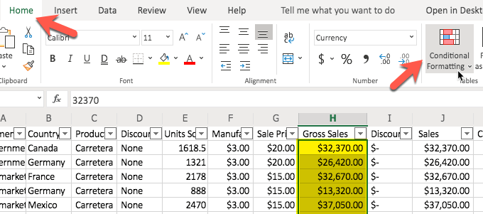
Conditional Formatting is handy if you want to highlight certain data. In this example, we are going to use our Excel Example file (with all of the financial data) and look for the “Gross Sales” that are over $25,000.
In order to do this, we first have to highlight the group of cells that we want evaluated. Now, keep in mind, you do not want to highlight the entire column or row. You only want to highlight just the cells that you want evaluated. Otherwise, the other cells (like headings) will also be evaluated and you would be surprised what Excel does with those headings (as an example).
So, we have our desired cells highlighted and now we click on the “Home” section/group and then “Conditional Formatting.”
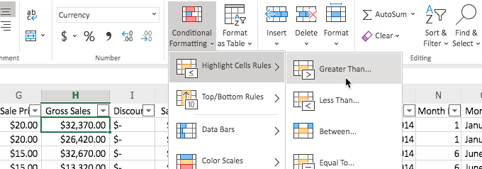
When we click on “Conditional Formatting” in the Ribbon, we have some options. In this case we want to highlight the cells that are greater than $25,000 so that is how we make our selection, as shown in the below image.
Now we will see a dialog box and we can type the value in the box. We type 25000. You don’t have to worry about commas or anything and in fact, it works better if you just type in the raw number.
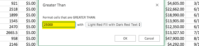
After we click “OK” we will see that the fields are automatically colored according to our choice (to the right) in our “Greater Than” above dialog box. In this case, “Light Red Fill with Dark Red Text). We could have chosen a different display option as well.
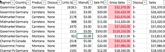
This conditional formatting is a great way to see, at a glance, data that is essential for one project or another. In this case, we could see the “Segments” (as they are referred to in the Excel Example file) that have been able to exceed $25,000 in Gross Sales.
Working With Formulas and Functions
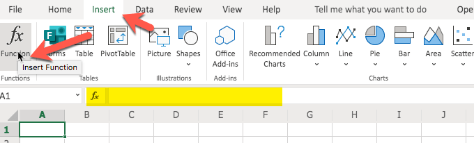
Learning how to use functions in Excel is very helpful. They are the basic guts of the formulas. If you want to see a listing of the functions to get an idea of what is available, click on the “Insert” menu/group and then at the far left, choose “Function/Functions.”
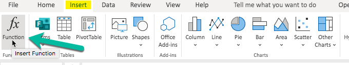
Even though the purpose of this button in the Excel Ribbon is to insert an actual function (which can also be accomplished by typing in the formula bar, starting with an equals sign and then starting to type the desired function), we can also use this to see what is available. You can scroll through the functions to get a sort of idea of what you can use in your formulas.
Granted, it is also very helpful to simply try them out and see what they do. You can select the group that you want to peruse by choosing a category, like “Commonly Used” for a shorter list of functions but a list that is often used (and for which some functions are covered in this article).
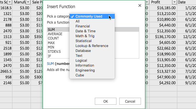
We will be using some of these functions in the examples of the formulas we discuss in this article.
The Equals = Sign
The equals sign ( = ) is very important in Excel. It plays an essential role. This is especially true in the cases of formulas. Basically, you don’t have a formula without preceding it with an equals sign. And without the formula, it is simply the data (or text) you have entered in that cell.
So just remember that before you are asking Excel to calculate or automate anything for you, that you type an equals sign ( = ) in the cell.

If you include a $ sign, that tells Excel not to move the formula. Normally, the auto adjustment of formulas (using what is called relative cell references), to changes in the worksheet, is a helpful thing but sometimes you may not want it and with that $ sign, you are able to tell Excel that. You simply insert the $ in front of the letter and number of the cell reference.
So a relative cell reference of D25 becomes $D$25. If this part is confusing, don’t worry about it. You can come back to it (or play with it with an Excel blank workbook).
The Awesome Ampersand >> &
The ampersand ( & ) is a fun little formula “tool,” allowing you to combine cells. For example, let’s say that you have a column for first names and another column for last names and you want to create a column for the full name. You can use the & to do just that.
Let’s try it in an Excel Worksheet. For this example, let’s use a blank sheet so we don’t interrupt any other project. Go ahead and type your first name in A1 and type your last name in B1. Now, to combine them, click your mouse on the C1 cell and type this formula: =A1 & “ “ & B1. Please only use the part in italics and not any of the rest of it (like not using the period).
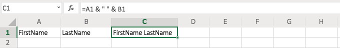
What do you see in C1? You should see your full name complete with a space between your first and last names, as would be normal in typing your full name. The & “ “ & portion of the formula is what produced that space. If you had not included “ “ you would have had your first name and last name without a space between them (go ahead and try it if you want to see the result).
Another similar formula uses CONCAT but we will learn about that a little later. For now, keep in mind what the ampersand ( & ) can do for you as this little tip comes in handy in many situations.
SUM() Function
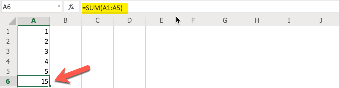
The SUM() function is very handy and it does just what it describes. It adds up the numbers you tell Excel to include and gives you the sum of their values. You can do this in a couple of different ways.
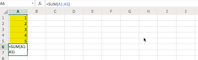
We started by typing in some numbers so we had some data to work with in the use of the function. We simply used 1, 2, 3, 4, 5 and started in A1 and typed in each cell going downward toward A5.
Now, to use the SUM() function, start by clicking in the desired cell, in this case we used A6, and typing =SUM( in the formula bar. In this example, stop when you get to the first “(.” Now, click in A1 (the top-most cell) and drag your mouse to A5 (or the bottom-most cell you want to include) and then return to the formula bar and type the closing “).” Do not include the periods or quotation marks and just the parentheses.
The other way to use this function is to manually type the information in the formula bar. This is especially helpful if you have quite a few numbers and scrolling to grab them is a bit difficult. Start this method the same way that you did for the example above, with “=SUM(.”
Then, type the top-most cell’s cell reference. In this case, that would be A1. Include a colon ( : ) and then type the bottom-most cell’s cell reference. In this case, that would be A5.
AVERAGE() Function
What if you wanted to figure out what the average of a group of numbers was? You can easily do that with the AVERAGE() function. You will notice, in the steps below, that it is basically the same as the SUM() function above but with a different function.
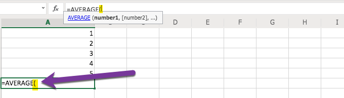
With that in mind, we start by selecting the cell we want to use for the result (in this case A6) and then start typing with an equals sign ( = ) and the word AVERAGE. You will notice that as you begin typing it you are offered suggestions and can click on AVERAGE instead of typing the full word, if you like.
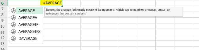
Ensure that you have an opening parenthesis in your formula before we add our cell range. Otherwise, you will receive an error.
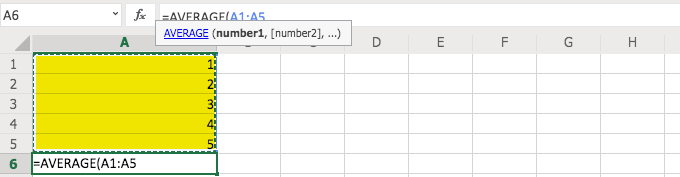
Now that we have “=AVERAGE(“ typed in our A6 cell (or whichever cell you are using for the result) we can select the cell range that we want to use. In this case we are using A1 through A5.
Keep in mind that you can also type it in manually rather than using the mouse to select the range. If you have a large data set typing in the range is probably easier than the scrolling that would be required to select it. But, of course, it is up to you.
To complete the process simply type in the closing parenthesis “)” and you will receive the average of the five numbers. As you can see, this process is very similar to the SUM() process and other functions. Once you get the hang of one function, the others will be easier.
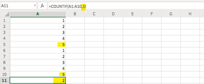
COUNTIF() Function
Let’s say we wanted to count how many times a certain number shows up in a data set. First, let’s prepare our file for this function so that we have something to count. Remove any formula that you may have in A6. Now, either copy A1 through A5 and paste starting in A6 or simply type the same numbers in the cells going downward starting with A6 and the value of 1 and then A7 with 2, etc.
Now, in A11 let’s start our function/formula. In this case, we are going to type “=COUNTIF(.” Then, we will select cells A1 through A10.
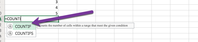
Be sure that you type or select “COUNTIF” and not one of the other COUNT-like functions or we will not get the same result.
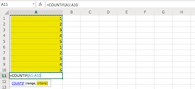
Before we do like we have with our other functions, and type the closing parenthesis “)” we need to answer the question of criteria and type that, after a comma “,” and before the parenthesis “).”
What is defined by the “criteria?” That is where we tell Excel what we want it to count (in this case). We typed a comma and then a “5” and then the closing parenthesis to obtain the count of the number of fives (5) that appear in the list of numbers. That result would be two (2) as there are two occurrences.
CONCAT or CONCANTENATE() Function
Similar to our example using just the ampersand ( & ) in our formula, you can combine cells using the CONCAT() function. Go ahead and try it, using our same example.
Type your first name in A1 and your last name in B1. Then, in C1 type CONCAT(A1, “ “ , B1).
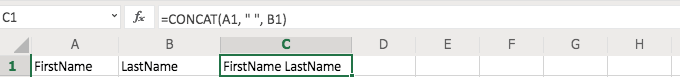
You will see that you get the same result as we did with the ampersand (&). Many people use the ampersand because it is easier and less cumbersome but now you see that you also have another option.
Note: This function may be CONCANTENATE in your version of Excel. Microsoft shortened the function name to just CONCAT and that tends to be easier to type (and remember) in the later versions of the software. Fortunately, if you start typing CONCA in your formula bar (after the equals sign), you will see which version your version of Excel uses and can select it by clicking on it with the mouse..
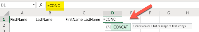
Remember that when you start to type it, to allow your version of Excel to reveal the correct function, to only type “CONCA” (or shorter) and not “CONCAN” (as the start for CONCANTENATE) or you may not see Excel’s suggestion since that is where the two functions start to differ.
Don’t be surprised if you prefer to use the merge method with the ampersand (&) instead of CONCAT(). That is normal.
If/Then Formulas
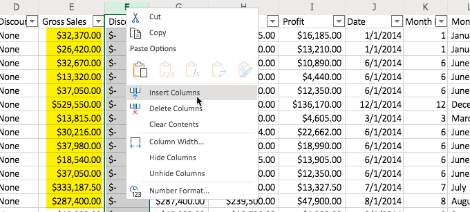
Let’s say we want to use an If/Then Formula to identify Discount (sort of a second discount) amount in a new column in our Example Excel file. In that case, first we start by adding a column and we are adding it after Column F and before Column G (again, in our downloaded example file).
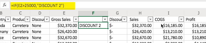
Now, we type in the formula. In this case, we type it in F2 and it is “=IF(E2>25000, “DISCOUNT 2”). This fulfills what the formula is looking for with a test (E2 greater than 25k) and then a result if the number in E2 passes that test (“DISCOUNT 2”).
Now, copy F2 and paste in the cells that follow it in the F column.
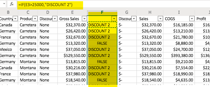
The formula will automatically adjust for each cell (relative cell referencing), with a reference to the appropriate cell. Remember that if you do not want it to automatically adjust, you can precede the cell alpha with a $ sign as well as the number, like A1 is $A$1.
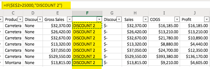
You can see, in the image above, that “DISCOUNT 2” appears in all of the cells in the F2 column. This is because the formula tells it to look at the E2 cell (represented by $E$2) and no relative cells. So, when the formula is copied to the next cell (i.e. F3) it is still looking at the E2 cell because of the dollar signs. So, all of the cells give the same result because they have the same formula referencing the same cell.
Also, if you want a value to show up instead of the word, “FALSE,” simply add a comma and then the word or number that you want to appear (text should be in quotes) at the end of the formula, before the ending parenthesis.
Pro Tip: Use VLOOKUP: Search and find a value in a different cell based on some matching text within the same row.
Managing Your Excel Projects
Fortunately, with the way that Excel documents are designed, you can do quite a bit with your Excel Workbooks. The ability to have different worksheets (tabs) in your document allows you to have related content all in one file. Also, if you feel that you are creating something that may have formulas that work better (or worse) you can copy (right-click option) your Worksheets (tabs) to have various versions of your Worksheet.
You can rename your tabs and use date codes to let you know which versions are the newest (or oldest). This is just one example of how you can use those tabs to your advantage in managing your Excel projects.
Here is an example of renaming your tabs in one of the later versions of Excel. You start by clicking on the tab and you get a result similar to the image here:
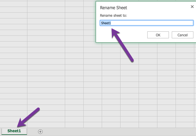

If you do not receive that response, that is ok. You may have an earlier version of Excel but it is somewhat intuitive in the way that it allows you to rename the tabs. You can right-click on the tab and get an option to “rename” in the earlier versions of Excel, as well, and sometimes simply type right in the tab.
Excel provides you with so many opportunities in your journey in learning how to use Excel. Now it is time to go out and use it! Have fun.
 |
|
A simple bar graph being created in Excel, running on Windows 11 |
|
| Developer(s) | Microsoft |
|---|---|
| Initial release | November 19, 1987; 35 years ago |
| Stable release |
2103 (16.0.13901.20400) |
| Written in | C++ (back-end)[2] |
| Operating system | Microsoft Windows |
| Type | Spreadsheet |
| License | Trialware[3] |
| Website | microsoft.com/en-us/microsoft-365/excel |
Excel for Mac (version 16.67), running on macOS Big Sur 11.5.2 |
|
| Developer(s) | Microsoft |
|---|---|
| Initial release | September 30, 1985; 37 years ago |
| Stable release |
16.70 (Build 23021201) |
| Written in | C++ (back-end), Objective-C (API/UI)[2] |
| Operating system | macOS |
| Type | Spreadsheet |
| License | Proprietary commercial software |
| Website | products.office.com/mac |
Excel for Android running on Android 13 |
|
| Developer(s) | Microsoft Corporation |
|---|---|
| Stable release |
16.0.14729.20146 |
| Operating system | Android Oreo and later |
| Type | Spreadsheet |
| License | Proprietary commercial software |
| Website | products.office.com/en-us/excel |
| Developer(s) | Microsoft Corporation |
|---|---|
| Stable release |
2.70.1 |
| Operating system | iOS 15 or later iPadOS 15 or later |
| Type | Spreadsheet |
| License | Proprietary commercial software |
| Website | products.office.com/en-us/excel |
Microsoft Excel is a spreadsheet developed by Microsoft for Windows, macOS, Android, iOS and iPadOS. It features calculation or computation capabilities, graphing tools, pivot tables, and a macro programming language called Visual Basic for Applications (VBA). Excel forms part of the Microsoft 365 suite of software.
Features
Basic operation
Microsoft Excel has the basic features of all spreadsheets,[7] using a grid of cells arranged in numbered rows and letter-named columns to organize data manipulations like arithmetic operations. It has a battery of supplied functions to answer statistical, engineering, and financial needs. In addition, it can display data as line graphs, histograms and charts, and with a very limited three-dimensional graphical display. It allows sectioning of data to view its dependencies on various factors for different perspectives (using pivot tables and the scenario manager).[8] A PivotTable is a tool for data analysis. It does this by simplifying large data sets via PivotTable fields. It has a programming aspect, Visual Basic for Applications, allowing the user to employ a wide variety of numerical methods, for example, for solving differential equations of mathematical physics,[9][10] and then reporting the results back to the spreadsheet. It also has a variety of interactive features allowing user interfaces that can completely hide the spreadsheet from the user, so the spreadsheet presents itself as a so-called application, or decision support system (DSS), via a custom-designed user interface, for example, a stock analyzer,[11] or in general, as a design tool that asks the user questions and provides answers and reports.[12][13] In a more elaborate realization, an Excel application can automatically poll external databases and measuring instruments using an update schedule,[14] analyze the results, make a Word report or PowerPoint slide show, and e-mail these presentations on a regular basis to a list of participants. Excel was not designed to be used as a database.[citation needed]
Microsoft allows for a number of optional command-line switches to control the manner in which Excel starts.[15]
Functions
Excel 2016 has 484 functions.[16] Of these, 360 existed prior to Excel 2010. Microsoft classifies these functions in 14 categories. Of the 484 current functions, 386 may be called from VBA as methods of the object «WorksheetFunction»[17] and 44 have the same names as VBA functions.[18]
With the introduction of LAMBDA, Excel will become Turing complete.[19]
Macro programming
VBA programming

Use of a user-defined function sq(x) in Microsoft Excel. The named variables x & y are identified in the Name Manager. The function sq is introduced using the Visual Basic editor supplied with Excel.

Subroutine in Excel calculates the square of named column variable x read from the spreadsheet, and writes it into the named column variable y.
The Windows version of Excel supports programming through Microsoft’s Visual Basic for Applications (VBA), which is a dialect of Visual Basic. Programming with VBA allows spreadsheet manipulation that is awkward or impossible with standard spreadsheet techniques. Programmers may write code directly using the Visual Basic Editor (VBE), which includes a window for writing code, debugging code, and code module organization environment. The user can implement numerical methods as well as automating tasks such as formatting or data organization in VBA[20] and guide the calculation using any desired intermediate results reported back to the spreadsheet.
VBA was removed from Mac Excel 2008, as the developers did not believe that a timely release would allow porting the VBA engine natively to Mac OS X. VBA was restored in the next version, Mac Excel 2011,[21] although the build lacks support for ActiveX objects, impacting some high level developer tools.[22]
A common and easy way to generate VBA code is by using the Macro Recorder.[23] The Macro Recorder records actions of the user and generates VBA code in the form of a macro. These actions can then be repeated automatically by running the macro. The macros can also be linked to different trigger types like keyboard shortcuts, a command button or a graphic. The actions in the macro can be executed from these trigger types or from the generic toolbar options. The VBA code of the macro can also be edited in the VBE. Certain features such as loop functions and screen prompt by their own properties, and some graphical display items, cannot be recorded but must be entered into the VBA module directly by the programmer. Advanced users can employ user prompts to create an interactive program, or react to events such as sheets being loaded or changed.
Macro Recorded code may not be compatible with Excel versions. Some code that is used in Excel 2010 cannot be used in Excel 2003. Making a Macro that changes the cell colors and making changes to other aspects of cells may not be backward compatible.
VBA code interacts with the spreadsheet through the Excel Object Model,[24] a vocabulary identifying spreadsheet objects, and a set of supplied functions or methods that enable reading and writing to the spreadsheet and interaction with its users (for example, through custom toolbars or command bars and message boxes). User-created VBA subroutines execute these actions and operate like macros generated using the macro recorder, but are more flexible and efficient.
History
From its first version Excel supported end-user programming of macros (automation of repetitive tasks) and user-defined functions (extension of Excel’s built-in function library). In early versions of Excel, these programs were written in a macro language whose statements had formula syntax and resided in the cells of special-purpose macro sheets (stored with file extension .XLM in Windows.) XLM was the default macro language for Excel through Excel 4.0.[25] Beginning with version 5.0 Excel recorded macros in VBA by default but with version 5.0 XLM recording was still allowed as an option. After version 5.0 that option was discontinued. All versions of Excel, including Excel 2021 are capable of running an XLM macro, though Microsoft discourages their use.[26]
Charts

Graph made using Microsoft Excel
Excel supports charts, graphs, or histograms generated from specified groups of cells. It also supports Pivot Charts that allow for a chart to be linked directly to a Pivot table. This allows the chart to be refreshed with the Pivot Table. The generated graphic component can either be embedded within the current sheet or added as a separate object.
These displays are dynamically updated if the content of cells changes. For example, suppose that the important design requirements are displayed visually; then, in response to a user’s change in trial values for parameters, the curves describing the design change shape, and their points of intersection shift, assisting the selection of the best design.
Add-ins
Additional features are available using add-ins. Several are provided with Excel, including:
- Analysis ToolPak: Provides data analysis tools for statistical and engineering analysis (includes analysis of variance and regression analysis)
- Analysis ToolPak VBA: VBA functions for Analysis ToolPak
- Euro Currency Tools: Conversion and formatting for euro currency
- Solver Add-In: Tools for optimization and equation solving
Data storage and communication
Number of rows and columns
Versions of Excel up to 7.0 had a limitation in the size of their data sets of 16K (214 = 16384) rows. Versions 8.0 through 11.0 could handle 64K (216 = 65536) rows and 256 columns (28 as label ‘IV’). Version 12.0 onwards, including the current Version 16.x, can handle over 1M (220 = 1048576) rows, and 16384 (214, labeled as column ‘XFD’) columns.[27]
File formats
| Filename extension |
.xls, (.xlsx, .xlsm, .xlsb — Excel 2007) |
|---|---|
| Internet media type |
application/vnd.ms-excel |
| Uniform Type Identifier (UTI) | com.microsoft.excel.xls |
| Developed by | Microsoft |
| Type of format | Spreadsheet |
Microsoft Excel up until 2007 version used a proprietary binary file format called Excel Binary File Format (.XLS) as its primary format.[28] Excel 2007 uses Office Open XML as its primary file format, an XML-based format that followed after a previous XML-based format called «XML Spreadsheet» («XMLSS»), first introduced in Excel 2002.[29]
Although supporting and encouraging the use of new XML-based formats as replacements, Excel 2007 remained backwards-compatible with the traditional, binary formats. In addition, most versions of Microsoft Excel can read CSV, DBF, SYLK, DIF, and other legacy formats. Support for some older file formats was removed in Excel 2007.[30] The file formats were mainly from DOS-based programs.
Binary
OpenOffice.org has created documentation of the Excel format. Two epochs of the format exist: the 97-2003 OLE format, and the older stream format.[31] Microsoft has made the Excel binary format specification available to freely download.[32]
XML Spreadsheet
The XML Spreadsheet format introduced in Excel 2002[29] is a simple, XML based format missing some more advanced features like storage of VBA macros. Though the intended file extension for this format is .xml, the program also correctly handles XML files with .xls extension. This feature is widely used by third-party applications (e.g. MySQL Query Browser) to offer «export to Excel» capabilities without implementing binary file format. The following example will be correctly opened by Excel if saved either as Book1.xml or Book1.xls:
<?xml version="1.0"?>
<Workbook xmlns="urn:schemas-microsoft-com:office:spreadsheet"
 xmlns:o="urn:schemas-microsoft-com:office:office"
 xmlns:x="urn:schemas-microsoft-com:office:excel"
 xmlns:ss="urn:schemas-microsoft-com:office:spreadsheet"
 xmlns:html="http://www.w3.org/TR/REC-html40">
 <Worksheet ss:Name="Sheet1">
  <Table ss:ExpandedColumnCount="2" ss:ExpandedRowCount="2" x:FullColumns="1" x:FullRows="1">
   <Row>
    <Cell><Data ss:Type="String">Name</Data></Cell>
    <Cell><Data ss:Type="String">Example</Data></Cell>
   </Row>
   <Row>
    <Cell><Data ss:Type="String">Value</Data></Cell>
    <Cell><Data ss:Type="Number">123</Data></Cell>
   </Row>
  </Table>
 </Worksheet>
</Workbook>
Current file extensions
Microsoft Excel 2007, along with the other products in the Microsoft Office 2007 suite, introduced new file formats. The first of these (.xlsx) is defined in the Office Open XML (OOXML) specification.
| Format | Extension | Description |
|---|---|---|
| Excel Workbook | .xlsx
|
The default Excel 2007 and later workbook format. In reality, a ZIP compressed archive with a directory structure of XML text documents. Functions as the primary replacement for the former binary .xls format, although it does not support Excel macros for security reasons. Saving as .xlsx offers file size reduction over .xls[33] |
| Excel Macro-enabled Workbook | .xlsm
|
As Excel Workbook, but with macro support. |
| Excel Binary Workbook | .xlsb
|
As Excel Macro-enabled Workbook, but storing information in binary form rather than XML documents for opening and saving documents more quickly and efficiently. Intended especially for very large documents with tens of thousands of rows, and/or several hundreds of columns. This format is very useful for shrinking large Excel files as is often the case when doing data analysis. |
| Excel Macro-enabled Template | .xltm
|
A template document that forms a basis for actual workbooks, with macro support. The replacement for the old .xlt format. |
| Excel Add-in | .xlam
|
Excel add-in to add extra functionality and tools. Inherent macro support because of the file purpose. |
Old file extensions
| Format | Extension | Description |
|---|---|---|
| Spreadsheet | .xls
|
Main spreadsheet format which holds data in worksheets, charts, and macros |
| Add-in (VBA) | .xla
|
Adds custom functionality; written in VBA |
| Toolbar | .xlb
|
The file extension where Microsoft Excel custom toolbar settings are stored. |
| Chart | .xlc
|
A chart created with data from a Microsoft Excel spreadsheet that only saves the chart. To save the chart and spreadsheet save as .XLS. XLC is not supported in Excel 2007 or in any newer versions of Excel. |
| Dialog | .xld
|
Used in older versions of Excel. |
| Archive | .xlk
|
A backup of an Excel Spreadsheet |
| Add-in (DLL) | .xll
|
Adds custom functionality; written in C++/C, Fortran, etc. and compiled in to a special dynamic-link library |
| Macro | .xlm
|
A macro is created by the user or pre-installed with Excel. |
| Template | .xlt
|
A pre-formatted spreadsheet created by the user or by Microsoft Excel. |
| Module | .xlv
|
A module is written in VBA (Visual Basic for Applications) for Microsoft Excel |
| Library | .DLL
|
Code written in VBA may access functions in a DLL, typically this is used to access the Windows API |
| Workspace | .xlw
|
Arrangement of the windows of multiple Workbooks |
Using other Windows applications
Windows applications such as Microsoft Access and Microsoft Word, as well as Excel can communicate with each other and use each other’s capabilities. The most common are Dynamic Data Exchange: although strongly deprecated by Microsoft, this is a common method to send data between applications running on Windows, with official MS publications referring to it as «the protocol from hell».[34] As the name suggests, it allows applications to supply data to others for calculation and display. It is very common in financial markets, being used to connect to important financial data services such as Bloomberg and Reuters.
OLE Object Linking and Embedding allows a Windows application to control another to enable it to format or calculate data. This may take on the form of «embedding» where an application uses another to handle a task that it is more suited to, for example a PowerPoint presentation may be embedded in an Excel spreadsheet or vice versa.[35][36][37][38]
Using external data
Excel users can access external data sources via Microsoft Office features such as (for example) .odc connections built with the Office Data Connection file format. Excel files themselves may be updated using a Microsoft supplied ODBC driver.
Excel can accept data in real-time through several programming interfaces, which allow it to communicate with many data sources such as Bloomberg and Reuters (through addins such as Power Plus Pro).
- DDE: «Dynamic Data Exchange» uses the message passing mechanism in Windows to allow data to flow between Excel and other applications. Although it is easy for users to create such links, programming such links reliably is so difficult that Microsoft, the creators of the system, officially refer to it as «the protocol from hell».[34] In spite of its many issues DDE remains the most common way for data to reach traders in financial markets.
- Network DDE Extended the protocol to allow spreadsheets on different computers to exchange data. Starting with Windows Vista, Microsoft no longer supports the facility.[39]
- Real Time Data: RTD although in many ways technically superior to DDE, has been slow to gain acceptance, since it requires non-trivial programming skills, and when first released was neither adequately documented nor supported by the major data vendors.[40][41]
Alternatively, Microsoft Query provides ODBC-based browsing within Microsoft Excel.[42][43][44]
Export and migration of spreadsheets
Programmers have produced APIs to open Excel spreadsheets in a variety of applications and environments other than Microsoft Excel. These include opening Excel documents on the web using either ActiveX controls, or plugins like the Adobe Flash Player. The Apache POI opensource project provides Java libraries for reading and writing Excel spreadsheet files.
Password protection
Microsoft Excel protection offers several types of passwords:
- Password to open a document[45]
- Password to modify a document[46]
- Password to unprotect the worksheet
- Password to protect workbook
- Password to protect the sharing workbook[47]
All passwords except password to open a document can be removed instantly regardless of the Microsoft Excel version used to create the document. These types of passwords are used primarily for shared work on a document. Such password-protected documents are not encrypted, and a data sources from a set password is saved in a document’s header. Password to protect workbook is an exception – when it is set, a document is encrypted with the standard password «VelvetSweatshop», but since it is known to the public, it actually does not add any extra protection to the document. The only type of password that can prevent a trespasser from gaining access to a document is password to open a document. The cryptographic strength of this kind of protection depends strongly on the Microsoft Excel version that was used to create the document.
In Microsoft Excel 95 and earlier versions, the password to open is converted to a 16-bit key that can be instantly cracked. In Excel 97/2000 the password is converted to a 40-bit key, which can also be cracked very quickly using modern equipment. As regards services that use rainbow tables (e.g. Password-Find), it takes up to several seconds to remove protection. In addition, password-cracking programs can brute-force attack passwords at a rate of hundreds of thousands of passwords a second, which not only lets them decrypt a document but also find the original password.
In Excel 2003/XP the encryption is slightly better – a user can choose any encryption algorithm that is available in the system (see Cryptographic Service Provider). Due to the CSP, an Excel file cannot be decrypted, and thus the password to open cannot be removed, though the brute-force attack speed remains quite high. Nevertheless, the older Excel 97/2000 algorithm is set by the default. Therefore, users who do not change the default settings lack reliable protection of their documents.
The situation changed fundamentally in Excel 2007, where the modern AES algorithm with a key of 128 bits started being used for decryption, and a 50,000-fold use of the hash function SHA1 reduced the speed of brute-force attacks down to hundreds of passwords per second. In Excel 2010, the strength of the protection by the default was increased two times due to the use of a 100,000-fold SHA1 to convert a password to a key.
Other platforms
Excel for mobile
Excel Mobile is a spreadsheet program that can edit XLSX files. It can edit and format text in cells, calculate formulas, search within the spreadsheet, sort rows and columns, freeze panes, filter the columns, add comments, and create charts. It cannot add columns or rows except at the edge of the document, rearrange columns or rows, delete rows or columns, or add spreadsheet tabs.[48][49][50][51][52][53] The 2007 version has the ability to use a full-screen mode to deal with limited screen resolution, as well as split panes to view different parts of a worksheet at one time.[51] Protection settings, zoom settings, autofilter settings, certain chart formatting, hidden sheets, and other features are not supported on Excel Mobile, and will be modified upon opening and saving a workbook.[52] In 2015, Excel Mobile became available for Windows 10 and Windows 10 Mobile on Windows Store.[54][55]
Excel for the web
Excel for the web is a free lightweight version of Microsoft Excel available as part of Office on the web, which also includes web versions of Microsoft Word and Microsoft PowerPoint.
Excel for the web can display most of the features available in the desktop versions of Excel, although it may not be able to insert or edit them. Certain data connections are not accessible on Excel for the web, including with charts that may use these external connections. Excel for the web also cannot display legacy features, such as Excel 4.0 macros or Excel 5.0 dialog sheets. There are also small differences between how some of the Excel functions work.[56]
Microsoft Excel Viewer
Microsoft Excel Viewer was a freeware program for Microsoft Windows for viewing and printing spreadsheet documents created by Excel.[57] Microsoft retired the viewer in April 2018 with the last security update released in February 2019 for Excel Viewer 2007 (SP3).[58][59]
The first version released by Microsoft was Excel 97 Viewer.[60][61] Excel 97 Viewer was supported in Windows CE for Handheld PCs.[62] In October 2004, Microsoft released Excel Viewer 2003.[63] In September 2007, Microsoft released Excel Viewer 2003 Service Pack 3 (SP3).[64] In January 2008, Microsoft released Excel Viewer 2007 (featuring a non-collapsible Ribbon interface).[65] In April 2009, Microsoft released Excel Viewer 2007 Service Pack 2 (SP2).[66] In October 2011, Microsoft released Excel Viewer 2007 Service Pack 3 (SP3).[67]
Microsoft advises to view and print Excel files for free to use the Excel Mobile application for Windows 10 and for Windows 7 and Windows 8 to upload the file to OneDrive and use Excel for the web with a Microsoft account to open them in a browser.[58][68]
Quirks
In addition to issues with spreadsheets in general, other problems specific to Excel include numeric precision, misleading statistics functions, mod function errors, date limitations and more.
Numeric precision
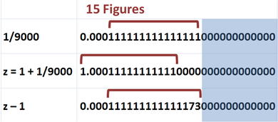
Excel maintains 15 figures in its numbers, but they are not always accurate: the bottom line should be the same as the top line.
Despite the use of 15-figure precision, Excel can display many more figures (up to thirty) upon user request. But the displayed figures are not those actually used in its computations, and so, for example, the difference of two numbers may differ from the difference of their displayed values. Although such departures are usually beyond the 15th decimal, exceptions do occur, especially for very large or very small numbers. Serious errors can occur if decisions are made based upon automated comparisons of numbers (for example, using the Excel If function), as equality of two numbers can be unpredictable.[citation needed]
In the figure, the fraction 1/9000 is displayed in Excel. Although this number has a decimal representation that is an infinite string of ones, Excel displays only the leading 15 figures. In the second line, the number one is added to the fraction, and again Excel displays only 15 figures. In the third line, one is subtracted from the sum using Excel. Because the sum in the second line has only eleven 1’s after the decimal, the difference when 1 is subtracted from this displayed value is three 0’s followed by a string of eleven 1’s. However, the difference reported by Excel in the third line is three 0’s followed by a string of thirteen 1’s and two extra erroneous digits. This is because Excel calculates with about half a digit more than it displays.
Excel works with a modified 1985 version of the IEEE 754 specification.[69] Excel’s implementation involves conversions between binary and decimal representations, leading to accuracy that is on average better than one would expect from simple fifteen digit precision, but that can be worse. See the main article for details.
Besides accuracy in user computations, the question of accuracy in Excel-provided functions may be raised. Particularly in the arena of statistical functions, Excel has been criticized for sacrificing accuracy for speed of calculation.[70][71]
As many calculations in Excel are executed using VBA, an additional issue is the accuracy of VBA, which varies with variable type and user-requested precision.[72]
Statistical functions
The accuracy and convenience of statistical tools in Excel has been criticized,[73][74][75][76][77] as mishandling missing data, as returning incorrect values due to inept handling of round-off and large numbers, as only selectively updating calculations on a spreadsheet when some cell values are changed, and as having a limited set of statistical tools. Microsoft has announced some of these issues are addressed in Excel 2010.[78]
Excel MOD function error
Excel has issues with modulo operations. In the case of excessively large results, Excel will return the error warning #NUM! instead of an answer.[79]
Fictional leap day in the year 1900
Excel includes February 29, 1900, incorrectly treating 1900 as a leap year, even though e.g. 2100 is correctly treated as a non-leap year.[80][81] The bug originated from Lotus 1-2-3 (deliberately implemented to save computer memory), and was also purposely implemented in Excel, for the purpose of bug compatibility.[82] This legacy has later been carried over into Office Open XML file format.[83]
Thus a (not necessarily whole) number greater than or equal to 61 interpreted as a date and time are the (real) number of days after December 30, 1899, 0:00, a non-negative number less than 60 is the number of days after December 31, 1899, 0:00, and numbers with whole part 60 represent the fictional day.
Date range
Excel supports dates with years in the range 1900–9999, except that December 31, 1899, can be entered as 0 and is displayed as 0-jan-1900.
Converting a fraction of a day into hours, minutes and days by treating it as a moment on the day January 1, 1900, does not work for a negative fraction.[84]
Conversion problems
Entering text that happens to be in a form that is interpreted as a date, the text can be unintentionally changed to a standard date format. A similar problem occurs when a text happens to be in the form of a floating-point notation of a number. In these cases the original exact text cannot be recovered from the result. Formatting the cell as TEXT before entering ambiguous text prevents Excel from converting to a date.
This issue has caused a well known problem in the analysis of DNA, for example in bioinformatics. As first reported in 2004,[85] genetic scientists found that Excel automatically and incorrectly converts certain gene names into dates. A follow-up study in 2016 found many peer reviewed scientific journal papers had been affected and that «Of the selected journals, the proportion of published articles with Excel files containing gene lists that are affected by gene name errors is 19.6 %.»[86] Excel parses the copied and pasted data and sometimes changes them depending on what it thinks they are. For example, MARCH1 (Membrane Associated Ring-CH-type finger 1) gets converted to the date March 1 (1-Mar) and SEPT2 (Septin 2) is converted into September 2 (2-Sep) etc.[87] While some secondary news sources[88] reported this as a fault with Excel, the original authors of the 2016 paper placed the blame with the researchers misusing Excel.[86][89]
In August 2020 the HUGO Gene Nomenclature Committee (HGNC) published new guidelines in the journal Nature regarding gene naming in order to avoid issues with «symbols that affect data handling and retrieval.» So far 27 genes have been renamed, including changing MARCH1 to MARCHF1 and SEPT1 to SEPTIN1 in order to avoid accidental conversion of the gene names into dates.[90]
Errors with large strings
The following functions return incorrect results when passed a string longer than 255 characters:[91]
type()incorrectly returns 16, meaning «Error value»IsText(), when called as a method of the VBA objectWorksheetFunction(i.e.,WorksheetFunction.IsText()in VBA), incorrectly returns «false».
Filenames
Microsoft Excel will not open two documents with the same name and instead will display the following error:
- A document with the name ‘%s’ is already open. You cannot open two documents with the same name, even if the documents are in different folders. To open the second document, either close the document that is currently open, or rename one of the documents.[92]
The reason is for calculation ambiguity with linked cells. If there is a cell ='[Book1.xlsx]Sheet1'!$G$33, and there are two books named «Book1» open, there is no way to tell which one the user means.[93]
Versions
Early history
Microsoft originally marketed a spreadsheet program called Multiplan in 1982. Multiplan became very popular on CP/M systems, but on MS-DOS systems it lost popularity to Lotus 1-2-3. Microsoft released the first version of Excel for the Macintosh on September 30, 1985, and the first Windows version was 2.05 (to synchronize with the Macintosh version 2.2) on November 19, 1987.[94][95] Lotus was slow to bring 1-2-3 to Windows and by the early 1990s, Excel had started to outsell 1-2-3 and helped Microsoft achieve its position as a leading PC software developer. This accomplishment solidified Microsoft as a valid competitor and showed its future of developing GUI software. Microsoft maintained its advantage with regular new releases, every two years or so.
Microsoft Windows
Excel 2.0 is the first version of Excel for the Intel platform. Versions prior to 2.0 were only available on the Apple Macintosh.
Excel 2.0 (1987)
The first Windows version was labeled «2» to correspond to the Mac version. It was announced on October 6, 1987, and released on November 19.[96] This included a run-time version of Windows.[97]
BYTE in 1989 listed Excel for Windows as among the «Distinction» winners of the BYTE Awards. The magazine stated that the port of the «extraordinary» Macintosh version «shines», with a user interface as good as or better than the original.
Excel 3.0 (1990)
Included toolbars, drawing capabilities, outlining, add-in support, 3D charts, and many more new features.[97]
Excel 4.0 (1992)
Introduced auto-fill.[98]
Also, an easter egg in Excel 4.0 reveals a hidden animation of a dancing set of numbers 1 through 3, representing Lotus 1-2-3, which is then crushed by an Excel logo.[99]
Excel 5.0 (1993)
With version 5.0, Excel has included Visual Basic for Applications (VBA), a programming language based on Visual Basic which adds the ability to automate tasks in Excel and to provide user-defined functions (UDF) for use in worksheets. VBA includes a fully featured integrated development environment (IDE). Macro recording can produce VBA code replicating user actions, thus allowing simple automation of regular tasks. VBA allows the creation of forms and in‑worksheet controls to communicate with the user. The language supports use (but not creation) of ActiveX (COM) DLL’s; later versions add support for class modules allowing the use of basic object-oriented programming techniques.
The automation functionality provided by VBA made Excel a target for macro viruses. This caused serious problems until antivirus products began to detect these viruses. Microsoft belatedly took steps to prevent the misuse by adding the ability to disable macros completely, to enable macros when opening a workbook or to trust all macros signed using a trusted certificate.
Versions 5.0 to 9.0 of Excel contain various Easter eggs, including a «Hall of Tortured Souls», a Doom-like minigame, although since version 10 Microsoft has taken measures to eliminate such undocumented features from their products.[100]
5.0 was released in a 16-bit x86 version for Windows 3.1 and later in a 32-bit version for NT 3.51 (x86/Alpha/PowerPC)
Excel 95 (v7.0)

Released in 1995 with Microsoft Office for Windows 95, this is the first major version after Excel 5.0, as there is no Excel 6.0 with all of the Office applications standardizing on the same major version number.
Internal rewrite to 32-bits. Almost no external changes, but faster and more stable.
Excel 95 contained a hidden Doom-like mini-game called «The Hall of Tortured Souls», a series of rooms featuring the names and faces of the developers as an easter egg.[101]
Excel 97 (v8.0)
Included in Office 97 (for x86 and Alpha). This was a major upgrade that introduced the paper clip office assistant and featured standard VBA used instead of internal Excel Basic. It introduced the now-removed Natural Language labels.
This version of Excel includes a flight simulator as an Easter Egg.
Excel 2000 (v9.0)

Included in Office 2000. This was a minor upgrade but introduced an upgrade to the clipboard where it can hold multiple objects at once. The Office Assistant, whose frequent unsolicited appearance in Excel 97 had annoyed many users, became less intrusive.
A small 3-D game called «Dev Hunter» (inspired by Spy Hunter) was included as an easter egg.[102][103]
Excel 2002 (v10.0)
Included in Office XP. Very minor enhancements.
Excel 2003 (v11.0)
Included in Office 2003. Minor enhancements.
Excel 2007 (v12.0)

Included in Office 2007. This release was a major upgrade from the previous version. Similar to other updated Office products, Excel in 2007 used the new Ribbon menu system. This was different from what users were used to, and was met with mixed reactions. One study reported fairly good acceptance by users except highly experienced users and users of word processing applications with a classical WIMP interface, but was less convinced in terms of efficiency and organization.[104] However, an online survey reported that a majority of respondents had a negative opinion of the change, with advanced users being «somewhat more negative» than intermediate users, and users reporting a self-estimated reduction in productivity.
Added functionality included Tables,[105] and the SmartArt set of editable business diagrams. Also added was an improved management of named variables through the Name Manager, and much-improved flexibility in formatting graphs, which allow (x, y) coordinate labeling and lines of arbitrary weight. Several improvements to pivot tables were introduced.
Also like other office products, the Office Open XML file formats were introduced, including .xlsm for a workbook with macros and .xlsx for a workbook without macros.[106]
Specifically, many of the size limitations of previous versions were greatly increased. To illustrate, the number of rows was now 1,048,576 (220) and columns was 16,384 (214; the far-right column is XFD). This changes what is a valid A1 reference versus a named range. This version made more extensive use of multiple cores for the calculation of spreadsheets; however, VBA macros are not handled in parallel and XLL add‑ins were only executed in parallel if they were thread-safe and this was indicated at registration.
Excel 2010 (v14.0)
Microsoft Excel 2010 running on Windows 7
Included in Office 2010, this is the next major version after v12.0, as version number 13 was skipped.
Minor enhancements and 64-bit support,[107] including the following:
- Multi-threading recalculation (MTR) for commonly used functions
- Improved pivot tables
- More conditional formatting options
- Additional image editing capabilities
- In-cell charts called sparklines
- Ability to preview before pasting
- Office 2010 backstage feature for document-related tasks
- Ability to customize the Ribbon
- Many new formulas, most highly specialized to improve accuracy[108]
Excel 2013 (v15.0)
Included in Office 2013, along with a lot of new tools included in this release:
- Improved Multi-threading and Memory Contention
- FlashFill[109]
- Power View[110]
- Power Pivot[111]
- Timeline Slicer
- Windows App
- Inquire[112]
- 50 new functions[113]
Excel 2016 (v16.0)
Included in Office 2016, along with a lot of new tools included in this release:
- Power Query integration
- Read-only mode for Excel
- Keyboard access for Pivot Tables and Slicers in Excel
- New Chart Types
- Quick data linking in Visio
- Excel forecasting functions
- Support for multiselection of Slicer items using touch
- Time grouping and Pivot Chart Drill Down
- Excel data cards[114]
Excel 2019, Excel 2021, Office 365 and subsequent (v16.0)
Microsoft no longer releases Office or Excel in discrete versions. Instead, features are introduced automatically over time using Windows Update. The version number remains 16.0. Thereafter only the approximate dates when features appear can now be given.
- Dynamic Arrays. These are essentially Array Formulas but they «Spill» automatically into neighboring cells and does not need the ctrl-shift-enter to create them. Further, dynamic arrays are the default format, with new «@» and «#» operators to provide compatibility with previous versions. This is perhaps the biggest structural change since 2007, and is in response to a similar feature in Google Sheets. Dynamic arrays started appearing in pre-releases about 2018, and as of March 2020 are available in published versions of Office 365 provided a user selected «Office Insiders».
Apple Macintosh

Microsoft Excel for Mac 2011
- 1985 Excel 1.0
- 1988 Excel 1.5
- 1989 Excel 2.2
- 1990 Excel 3.0
- 1992 Excel 4.0
- 1993 Excel 5.0 (part of Office 4.x—Final Motorola 680×0 version[115] and first PowerPC version)
- 1998 Excel 8.0 (part of Office 98)
- 2000 Excel 9.0 (part of Office 2001)
- 2001 Excel 10.0 (part of Office v. X)
- 2004 Excel 11.0 (part of Office 2004)
- 2008 Excel 12.0 (part of Office 2008)
- 2010 Excel 14.0 (part of Office 2011)
- 2015 Excel 15.0 (part of Office 2016—Office 2016 for Mac brings the Mac version much closer to parity with its Windows cousin, harmonizing many of the reporting and high-level developer functions, while bringing the ribbon and styling into line with its PC counterpart.)[116]
OS/2
- 1989 Excel 2.2
- 1990 Excel 2.3
- 1991 Excel 3.0
Summary
| Legend: | Old version, not maintained | Older version, still maintained | Current stable version |
|---|
| Year | Name | Version | Comments |
|---|---|---|---|
| 1987 | Excel 2 | 2.0 | Renumbered to 2 to correspond with contemporary Macintosh version. Supported macros (later known as Excel 4 macros). |
| 1990 | Excel 3 | 3.0 | Added 3D graphing capabilities |
| 1992 | Excel 4 | 4.0 | Introduced auto-fill feature |
| 1993 | Excel 5 | 5.0 | Included Visual Basic for Applications (VBA) and various object-oriented options |
| 1995 | Excel 95 | 7.0 | Renumbered for contemporary Word version. Both programs were packaged in Microsoft Office by this time. |
| 1997 | Excel 97 | 8.0 | |
| 2000 | Excel 2000 | 9.0 | Part of Microsoft Office 2000, which was itself part of Windows Millennium (also known as «Windows ME»). |
| 2002 | Excel 2002 | 10.0 | |
| 2003 | Excel 2003 | 11.0 | Released only 1 year later to correspond better with the rest of Microsoft Office (Word, PowerPoint, etc.). |
| 2007 | Excel 2007 | 12.0 | |
| 2010 | Excel 2010 | 14.0 | Due to superstitions surrounding the number 13, Excel 13 was skipped in version counting. |
| 2013 | Excel 2013 | 15.0 | Introduced 50 more mathematical functions (available as pre-packaged commands, rather than typing the formula manually). |
| 2016 | Excel 2016 | 16.0 | Part of Microsoft Office 2016 |
| Year | Name | Version | Comments |
|---|---|---|---|
| 1985 | Excel 1 | 1.0 | Initial version of Excel. Supported macros (later known as Excel 4 macros). |
| 1988 | Excel 1.5 | 1.5 | |
| 1989 | Excel 2 | 2.2 | |
| 1990 | Excel 3 | 3.0 | |
| 1992 | Excel 4 | 4.0 | |
| 1993 | Excel 5 | 5.0 | Only available on PowerPC-based Macs. First PowerPC version. |
| 1998 | Excel 98 | 8.0 | Excel 6 and Excel 7 were skipped to correspond with the rest of Microsoft Office at the time. |
| 2000 | Excel 2000 | 9.0 | |
| 2001 | Excel 2001 | 10.0 | |
| 2004 | Excel 2004 | 11.0 | |
| 2008 | Excel 2008 | 12.0 | |
| 2011 | Excel 2011 | 14.0 | As with the Windows version, version 13 was skipped for superstitious reasons. |
| 2016 | Excel 2016 | 16.0 | As with the rest of Microsoft Office, so it is for Excel: Future release dates for the Macintosh version are intended to correspond better to those for the Windows version, from 2016 onward. |
| Year | Name | Version | Comments |
|---|---|---|---|
| 1989 | Excel 2.2 | 2.2 | Numbered in between Windows versions at the time |
| 1990 | Excel 2.3 | 2.3 | |
| 1991 | Excel 3 | 3.0 | Last OS/2 version. Discontinued subseries of Microsoft Excel, which is otherwise still an actively developed program. |
Impact
Excel offers many user interface tweaks over the earliest electronic spreadsheets; however, the essence remains the same as in the original spreadsheet software, VisiCalc: the program displays cells organized in rows and columns, and each cell may contain data or a formula, with relative or absolute references to other cells.
Excel 2.0 for Windows, which was modeled after its Mac GUI-based counterpart, indirectly expanded the installed base of the then-nascent Windows environment. Excel 2.0 was released a month before Windows 2.0, and the installed base of Windows was so low at that point in 1987 that Microsoft had to bundle a runtime version of Windows 1.0 with Excel 2.0.[117] Unlike Microsoft Word, there never was a DOS version of Excel.
Excel became the first spreadsheet to allow the user to define the appearance of spreadsheets (fonts, character attributes, and cell appearance). It also introduced intelligent cell re-computation, where only cells dependent on the cell being modified are updated (previous spreadsheet programs recomputed everything all the time or waited for a specific user command). Excel introduced auto-fill, the ability to drag and expand the selection box to automatically copy a cell or row contents to adjacent cells or rows, adjusting the copies intelligently by automatically incrementing cell references or contents. Excel also introduced extensive graphing capabilities.
Security
Because Excel is widely used, it has been attacked by hackers. While Excel is not directly exposed to the Internet, if an attacker can get a victim to open a file in Excel, and there is an appropriate security bug in Excel, then the attacker can gain control of the victim’s computer.[118] UK’s GCHQ has a tool named TORNADO ALLEY with this purpose.[119][120]
Games
Besides the easter eggs, numerous games have been created or recreated in Excel, such as Tetris, 2048, Scrabble, Yahtzee, Angry Birds, Pac-Man, Civilization, Monopoly, Battleship, Blackjack, Space Invaders, and others.[121][122][123][124][125]
In 2020, Excel became an esport with the advent of the Financial Modeling World Cup.[126]
See also
- Comparison of spreadsheet software
- Numbers (spreadsheet)—the iWork equivalent
- Spreadmart
- Financial Modeling World Cup, online esport financial modelling competition using Excel
References
- ^ «Update history for Microsoft Office 2019». Microsoft Docs. Retrieved April 13, 2021.
- ^ a b «C++ in MS Office». cppcon. July 17, 2014. Archived from the original on November 7, 2019. Retrieved June 25, 2019.
- ^ «Microsoft Office Excel 365». Microsoft.com. Retrieved January 25, 2021.
- ^ «Update history for Office for Mac». Microsoft Docs.
- ^ «Microsoft Excel APKs». APKMirror.
- ^ «Microsoft Excel». App Store.
- ^
Harvey, Greg (2006). Excel 2007 For Dummies (1st ed.). Wiley. ISBN 978-0-470-03737-9. - ^
Harvey, Greg (2007). Excel 2007 Workbook for Dummies (2nd ed.). Wiley. p. 296 ff. ISBN 978-0-470-16937-7. - ^
de Levie, Robert (2004). Advanced Excel for scientific data analysis. Oxford University Press. ISBN 978-0-19-515275-3. - ^
Bourg, David M. (2006). Excel scientific and engineering cookbook. O’Reilly. ISBN 978-0-596-00879-6. - ^
Şeref, Michelle M. H. & Ahuja, Ravindra K. (2008). «§4.2 A portfolio management and optimization spreadsheet DSS». In Burstein, Frad & Holsapple, Clyde W. (eds.). Handbook on Decision Support Systems 1: Basic Themes. Springer. ISBN 978-3-540-48712-8. - ^
Wells, Eric & Harshbarger, Steve (1997). Microsoft Excel 97 Developer’s Handbook. Microsoft Press. ISBN 978-1-57231-359-0. Excellent examples are developed that show just how applications can be designed. - ^
Harnett, Donald L. & Horrell, James F. (1998). Data, statistics, and decision models with Excel. Wiley. ISBN 978-0-471-13398-8. - ^
Some form of data acquisition hardware is required. See, for example, Austerlitz, Howard (2003). Data acquisition techniques using PCs (2nd ed.). Academic Press. p. 281 ff. ISBN 978-0-12-068377-2. - ^
«Description of the startup switches for Excel». Microsoft Help and Support. Microsoft Support. May 7, 2007. Retrieved December 14, 2010.Microsoft Excel accepts a number of optional switches that you can use to control how the program starts. This article lists the switches and provides a description of each switch.
{{cite web}}: CS1 maint: url-status (link) - ^ «Excel functions (alphabetical)». microsoft.com. Microsoft. Retrieved November 4, 2018.
{{cite web}}: CS1 maint: url-status (link) - ^ «WorksheetFunction Object (Excel)». Office VBA Reference. Microsoft. March 30, 2022. Retrieved November 4, 2018.
{{cite web}}: CS1 maint: url-status (link) - ^ «Functions (Visual Basic for Applications)». Office VBA Reference. Microsoft. September 13, 2021. Retrieved November 4, 2018.
{{cite web}}: CS1 maint: url-status (link) - ^ Gordon, Andy (January 25, 2021). «LAMBDA: The ultimate Excel worksheet function». microsoft.com. Microsoft. Retrieved April 23, 2021.
{{cite web}}: CS1 maint: url-status (link) - ^
For example, by converting to Visual Basic the recipes in Press, William H. Press; Teukolsky, Saul A.; Vetterling, William T. & Flannery, Brian P. (2007). Numerical recipes: the art of scientific computing (3rd ed.). Cambridge University Press. ISBN 978-0-521-88068-8. Code conversion to Basic from Fortran probably is easier than from C++, so the 2nd edition (ISBN 0521437210) may be easier to use, or the Basic code implementation of the first edition: Sprott, Julien C. (1991). Numerical recipes: routines and examples in BASIC. Cambridge University Press. ISBN 978-0-521-40689-5. - ^ «Excel». Office for Mac. OfficeforMacHelp.com. Archived from the original on June 19, 2012. Retrieved July 8, 2012.
- ^ «Using Excel — PC or Mac? | Excel Lemon». www.excellemon.com. Archived from the original on September 21, 2016. Retrieved July 29, 2015.
- ^ However an increasing proportion of Excel functionality is not captured by the Macro Recorder leading to largely useless macros. Compatibility among multiple versions of Excel is also a downfall of this method. A macro recorder in Excel 2010 may not work in Excel 2003 or older. This is most common when changing colors and formatting of cells.
Walkenbach, John (2007). «Chapter 6: Using the Excel macro recorder». Excel 2007 VBA Programming for Dummies (Revised by Jan Karel Pieterse ed.). Wiley. p. 79 ff. ISBN 978-0-470-04674-6. - ^ Walkenbach, John (February 2, 2007). «Chapter 4: Introducing the Excel object model». cited work. p. 53 ff. ISBN 978-0-470-04674-6.
- ^ «The Spreadsheet Page for Excel Users and Developers». spreadsheetpage.com. J-Walk & Associates, Inc. Retrieved December 19, 2012.
- ^ «Working with Excel 4.0 macros». microsoft.com. Microsoft Office Support. Retrieved December 19, 2012.
- ^ «The «Big Grid» and Increased Limits in Excel 2007″. microsoft.com. May 23, 2014. Retrieved April 10, 2008.
{{cite web}}: CS1 maint: url-status (link) - ^ «How to extract information from Office files by using Office file formats and schemas». microsoft.com. Microsoft. February 26, 2008. Retrieved November 10, 2008.
{{cite web}}: CS1 maint: url-status (link) - ^ a b «XML Spreadsheet Reference». Microsoft Excel 2002 Technical Articles. MSDN. August 2001. Retrieved November 10, 2008.
- ^ «Deprecated features for Excel 2007». Microsoft—David Gainer. August 24, 2006. Retrieved January 2, 2009.
- ^ «OpenOffice.org’s documentation of the Microsoft Excel File Format» (PDF). August 2, 2008.
- ^ «Microsoft Office Excel 97 — 2007 Binary File Format Specification (*.xls 97-2007 format)». Microsoft Corporation. 2007.
- ^ Fairhurst, Danielle Stein (March 17, 2015). Using Excel for Business Analysis: A Guide to Financial Modelling Fundamentals. John Wiley & Sons. ISBN 978-1-119-06245-5.
- ^ a b Newcomer, Joseph M. «Faking DDE with Private Servers». Dr. Dobb’s.
- ^ Schmalz, Michael (2006). «Chapter 5: Using Access VBA to automate Excel». Integrating Excel and Access. O’Reilly Media, Inc. ISBN 978-0-596-00973-1.Schmalz, Michael (2006). «Chapter 5: Using Access VBA to automate Excel». Integrating Excel and Access. O’Reilly Media, Inc. ISBN 978-0-596-00973-1.
- ^ Cornell, Paul (2007). «Chapter 5: Connect to other databases». Excel as Your Database. Apress. p. 117 ff. ISBN 978-1-59059-751-4.
- ^ DeMarco, Jim (2008). «Excel’s data import tools». Pro Excel 2007 VBA. Apress. p. 43 ff. ISBN 978-1-59059-957-0.
- ^
Harts, Doug (2007). «Importing Access data into Excel 2007». Microsoft Office 2007 Business Intelligence: Reporting, Analysis, and Measurement from the Desktop. McGraw-Hill Professional. ISBN 978-0-07-149424-3. - ^ «About Network DDE — Win32 apps». learn.microsoft.com.
- ^ «How to set up and use the RTD function in Excel — Office». learn.microsoft.com.
- ^
DeMarco, Jim (2008). Pro Excel 2007 VBA. Berkeley, CA: Apress. p. 225. ISBN 978-1-59059-957-0.External data is accessed through a connection file, such as an Office Data Connection (ODC) file (.odc)
- ^
Bullen, Stephen; Bovey, Rob & Green, John (2009). Professional Excel Development (2nd ed.). Upper Saddle River, NJ: Addison-Wesley. p. 665. ISBN 978-0-321-50879-9.To create a robust solution, we always have to include some VBA code …
- ^ William, Wehrs (2000). «An Applied DSS Course Using Excel and VBA: IS and/or MS?» (PDF). The Proceedings of ISECON (Information System Educator Conference). p. 4. Archived from the original (PDF) on August 21, 2010. Retrieved February 5, 2010.
Microsoft Query is a data retrieval tool (i.e. ODBC browser) that can be employed within Excel 97. It allows a user to create and save queries on external relational databases for which an ODBC driver is available.
- ^ Use Microsoft Query to retrieve external data Archived March 12, 2010, at the Wayback Machine
- ^ «Password protect documents, workbooks, and presentations — Word — Office.com». Office.microsoft.com. Retrieved April 24, 2013.
- ^ «Password protect documents, workbooks, and presentations — Word — Office.com». Office.microsoft.com. Retrieved April 24, 2013.
- ^ «Password protect worksheet or workbook elements — Excel — Office.com». Office.microsoft.com. Archived from the original on March 26, 2013. Retrieved April 24, 2013.
- ^ Ralph, Nate. «Office for Windows Phone 8: Your handy starter guide». TechHive. Archived from the original on October 15, 2014. Retrieved August 30, 2014.
- ^ Wollman, Dana. «Microsoft Office Mobile for iPhone hands-on». Engadget. Retrieved August 30, 2014.
- ^ Pogue, David. «Microsoft Adds Office for iPhone. Yawn». The New York Times. Retrieved August 30, 2014.
- ^ a b Ogasawara, Todd. «What’s New in Excel Mobile». Microsoft. Archived from the original on February 8, 2008. Retrieved September 13, 2007.
- ^ a b «Unsupported features in Excel Mobile». Microsoft. Archived from the original on October 20, 2007. Retrieved September 21, 2007.
- ^ Use Excel Mobile Archived October 20, 2007, at the Wayback Machine. Microsoft. Retrieved September 21, 2007.
- ^ «Excel Mobile». Windows Store. Microsoft. Retrieved June 26, 2016.
- ^ «PowerPoint Mobile». Windows Store. Microsoft. Retrieved June 26, 2016.
- ^ «Differences between using a workbook in the browser and in Excel — Office Support». support.office.com. Archived from the original on 8 February 2017. Retrieved 7 February 2017.
- ^ «Description of the Excel Viewer». Microsoft. February 17, 2012. Archived from the original on April 6, 2013.
- ^ a b «How to obtain the latest Excel Viewer». Microsoft Docs. May 22, 2020. Retrieved January 3, 2021.
- ^ «Description of the security update for Excel Viewer 2007: February 12, 2019». Microsoft. April 16, 2020. Retrieved January 3, 2021.
- ^ «Microsoft Excel Viewer». Microsoft. 1997. Archived from the original on January 20, 1998.
- ^ «Excel 97/2000 Viewer: Spreadsheet Files». Microsoft. Archived from the original on January 13, 2004.
- ^ «New Features in Windows CE .NET 4.1». Microsoft Docs. June 30, 2006. Retrieved January 3, 2021.
- ^ «Excel Viewer 2003». Microsoft. October 12, 2004. Archived from the original on January 15, 2005.
- ^ «Excel Viewer 2003 Service Pack 3 (SP3)». Microsoft. September 17, 2007. Archived from the original on October 11, 2007.
- ^ «Excel Viewer». Microsoft. January 14, 2008. Archived from the original on September 26, 2010.
- ^ «Excel Viewer 2007 Service Pack 2 (SP2)». Microsoft. April 24, 2009. Archived from the original on April 28, 2012.
- ^ «Excel Viewer 2007 Service Pack 3 (SP3)». Microsoft. October 25, 2011. Archived from the original on December 29, 2011.
- ^ «Supported versions of the Office viewers». Microsoft. April 16, 2020. Retrieved January 3, 2021.
- ^
Microsoft’s overview is found at: «Floating-point arithmetic may give inaccurate results in Excel». Revision 8.2 ; article ID: 78113. Microsoft support. June 30, 2010. Retrieved July 2, 2010. - ^
Altman, Micah; Gill, Jeff; McDonald, Michael (2004). «§2.1.1 Revealing example: Computing the coefficient standard deviation». Numerical issues in statistical computing for the social scientist. Wiley-IEEE. p. 12. ISBN 978-0-471-23633-7. - ^ de Levie, Robert (2004). cited work. pp. 45–46. ISBN 978-0-19-515275-3.
- ^
Walkenbach, John (2010). «Defining data types». Excel 2010 Power Programming with VBA. Wiley. pp. 198 ff and Table 8–1. ISBN 978-0-470-47535-5. - ^ McCullough, Bruce D.; Wilson, Berry (2002). «On the accuracy of statistical procedures in Microsoft Excel 2000 and Excel XP». Computational Statistics & Data Analysis. 40 (4): 713–721. doi:10.1016/S0167-9473(02)00095-6.
- ^ McCullough, Bruce D.; Heiser, David A. (2008). «On the accuracy of statistical procedures in Microsoft Excel 2007». Computational Statistics & Data Analysis. 52 (10): 4570–4578. CiteSeerX 10.1.1.455.5508. doi:10.1016/j.csda.2008.03.004.
- ^ Yalta, A. Talha (2008). «The accuracy of statistical distributions in Microsoft Excel 2007». Computational Statistics & Data Analysis. 52 (10): 4579–4586. doi:10.1016/j.csda.2008.03.005.
- ^ Goldwater, Eva. «Using Excel for Statistical Data Analysis—Caveats». University of Massachusetts School of Public Health. Retrieved November 10, 2008.
- ^
Heiser, David A. (2008). «Microsoft Excel 2000, 2003 and 2007 faults, problems, workarounds and fixes». Archived from the original on April 18, 2010. Retrieved April 8, 2010. - ^
Function improvements in Excel 2010 Archived April 6, 2010, at the Wayback Machine Comments are provided from readers that may illuminate some remaining problems. - ^ «The MOD bug». Byg Software. Archived from the original on January 11, 2016. Retrieved November 10, 2008.
- ^ «Days of the week before March 1, 1900 are incorrect in Excel». Microsoft. Archived from the original on July 14, 2012. Retrieved November 10, 2008.
- ^ «Excel incorrectly assumes that the year 1900 is a leap year». Microsoft. Retrieved May 1, 2019.
- ^ Spolsky, Joel (June 16, 2006). «My First BillG Review». Joel on Software. Retrieved November 10, 2008.
- ^ «The Contradictory Nature of OOXML». ConsortiumInfo.org. January 17, 2007.
- ^ «Negative date and time value are displayed as pound signs (###) in Excel». Microsoft. Retrieved March 26, 2012.
- ^ Zeeberg, Barry R; Riss, Joseph; Kane, David W; Bussey, Kimberly J; Uchio, Edward; Linehan, W Marston; Barrett, J Carl; Weinstein, John N (2004). «Mistaken Identifiers: Gene name errors can be introduced inadvertently when using Excel in bioinformatics». BMC Bioinformatics. 5 (1): 80. doi:10.1186/1471-2105-5-80. PMC 459209. PMID 15214961.
- ^ a b Ziemann, Mark; Eren, Yotam; El-Osta, Assam (2016). «Gene name errors are widespread in the scientific literature». Genome Biology. 17 (1): 177. doi:10.1186/s13059-016-1044-7. PMC 4994289. PMID 27552985.
- ^ Anon (2016). «Microsoft Excel blamed for gene study errors». bbc.co.uk. London: BBC News.
- ^ Cimpanu, Catalin (August 24, 2016). «One in Five Scientific Papers on Genes Contains Errors Because of Excel». Softpedia. SoftNews.
- ^ Ziemann, Mark (2016). «Genome Spot: My personal thoughts on gene name errors». genomespot.blogspot.co.uk. Archived from the original on August 30, 2016.
- ^ Vincent, James (August 6, 2020). «Scientists rename human genes to stop Microsoft Excel from misreading them as dates». The Verge. Retrieved October 9, 2020.
- ^ «Excel: type() and
WorksheetFunction.IsText()fail for long strings». Stack Overflow. November 3, 2018. - ^ Rajah, Gary (August 2, 2004). «Trouble with macros». The Hindu Business Line. Retrieved March 19, 2019.
- ^ Chirilov, Joseph (January 8, 2009). «Microsoft Excel — Why Can’t I Open Two Files With the Same Name?». MSDN Blogs. Microsoft Corporation. Archived from the original on July 29, 2010. Retrieved March 19, 2019.
- ^ Infoworld Media Group, Inc. (July 7, 1986). InfoWorld First Look: Supercalc 4 challenging 1-2-3 with new tactic.
- ^ «The History of Microsoft — 1987». channel9.msdn.com. Archived from the original on September 27, 2010. Retrieved October 7, 2022.
- ^ «The History of Microsoft — 1987». learn.microsoft.com. Retrieved October 7, 2022.
- ^ a b Walkenbach, John (December 4, 2013). «Excel Version History». The Spreadsheet Page. John Walkenbach. Retrieved July 12, 2020.
- ^ Lewallen, Dale (1992). PC/Computing guide to Excel 4.0 for Windows. Ziff Davis. p. 13. ISBN 9781562760489. Retrieved July 27, 2013.
- ^ Lake, Matt (April 6, 2009). «Easter Eggs we have loved: Excel 4». crashreboot.blogspot.com. Retrieved November 5, 2013.
- ^ Osterman, Larry (October 21, 2005). «Why no Easter Eggs?». Larry Osterman’s WebLog. MSDN Blogs. Retrieved July 29, 2006.
- ^ «Excel 95 Hall of Tortured Souls». Retrieved July 7, 2006.
- ^ «Excel Oddities: Easter Eggs». Archived from the original on August 21, 2006. Retrieved August 10, 2006.
- ^ «Car Game In Ms Excel». Totalchoicehosting.com. September 6, 2005. Retrieved January 28, 2014.
- ^ Dostál, M (December 9, 2010). User Acceptance of the Microsoft Ribbon User Interface (PDF). Palacký University of Olomouc. ISBN 978-960-474-245-5. ISSN 1792-6157. Retrieved May 28, 2013.
- ^ [Using Excel Tables to
Manipulate Billing Data https://mooresolutionsinc.com/downloads/Billing_MJ12.pdf] - ^ Dodge, Mark; Stinson, Craig (2007). «Chapter 1: What’s new in Microsoft Office Excel 2007». Microsoft Office Excel 2007 inside out. Microsoft Press. p. 1 ff. ISBN 978-0-7356-2321-7.
- ^ «What’s New in Excel 2010 — Excel». Archived from the original on December 2, 2013. Retrieved September 23, 2010.
- ^ Walkenbach, John (2010). «Some Essential Background». Excel 2010 Power Programming with VBA. Indianapolis, Indiana: Wiley Publishing, Inc. p. 20. ISBN 9780470475355.
- ^ Harris, Steven (October 1, 2013). «Excel 2013 — Flash Fill». Experts-Exchange.com. Experts Exchange. Retrieved November 23, 2013.
- ^ «What’s new in Excel 2013». Office.com. Microsoft. Retrieved January 25, 2014.
- ^ K., Gasper (October 10, 2013). «Does a PowerPivot Pivot Table beat a regular Pivot Table». Experts-Exchange.com. Experts Exchange. Retrieved November 23, 2013.
- ^ K., Gasper (May 20, 2013). «Inquire Add-In for Excel 2013». Experts-Exchange.com. Experts Exchange. Retrieved November 23, 2013.
- ^ «New functions in Excel 2013». Office.com. Microsoft. Retrieved November 23, 2013.
- ^ «What’s new in Office 2016». Office.com. Microsoft. Retrieved August 16, 2015.
- ^ «Microsoft Announces March Availability of Office 98 Macintosh Edition». Microsoft. January 6, 1998. Retrieved December 29, 2017.
- ^ «Office for Mac Is Finally a ‘First-Class Citizen’«. Re/code. July 16, 2015. Retrieved July 29, 2015.
- ^ Perton, Marc (November 20, 2005). «Windows at 20: 20 things you didn’t know about Windows 1.0». switched.com. Archived from the original on April 11, 2013. Retrieved August 1, 2013.
- ^ Keizer, Gregg (February 24, 2009). «Attackers exploit unpatched Excel vulnerability». Computerworld. IDG Communications, Inc. Retrieved March 19, 2019.
- ^ «JTRIG Tools and Techniques». The Intercept. First Look Productions, Inc. July 14, 2014. Archived from the original on July 14, 2014. Retrieved March 19, 2019.
- ^ Cook, John. «JTRIG Tools and Techniques». The Intercept. p. 4. Retrieved March 19, 2019 – via DocumentCloud.
- ^ Phillips, Gavin (December 11, 2015). «8 Legendary Games Recreated in Microsoft Excel». MUO.
- ^ «Excel Games – Fun Things to Do With Spreadsheets». November 10, 2021.
- ^ «Unusual Uses of Excel». techcommunity.microsoft.com. August 5, 2022.
- ^ «Someone made a version of ‘Civilization’ that runs in Microsoft Excel». Engadget.
- ^ Dalgleish, Debra. «Have Fun Playing Games in Excel». Contextures Excel Tips.
- ^ «Microsoft Excel esports is real and it already has an international tournament». ONE Esports. June 9, 2021.
References
- Bullen, Stephen; Bovey, Rob; Green, John (2009). Professional Excel Development: The Definitive Guide to Developing Applications Using Microsoft Excel and VBA (2nd ed.). Boston: Addison Wesley. ISBN 978-0-321-50879-9.
- Dodge, Mark; Stinson, Craig (2007). Microsoft Office Excel 2007 Inside Out. Redmond, Wash.: Microsoft Press. ISBN 978-0-7356-2321-7.
- Billo, E. Joseph (2011). Excel for Chemists: A Comprehensive Guide (3rd ed.). Hoboken, N.J.: John Wiley & Sons. ISBN 978-0-470-38123-6.
- Gordon, Andy (January 25, 2021). «LAMBDA: The ultimate Excel worksheet function». microsoft.com. Microsoft. Retrieved April 23, 2021.
External links
![]()
Wikibooks has a book on the topic of: Excel
- Microsoft Excel – official site
The best way to learn about Excel 2013 is to start using it. Create a blank workbook and learn the basics of working with columns, cells, and data.
Start using Excel
-
The best way to learn about Excel 2013 is to start using it.
-
You can open an existing workbook, or start with a template. Then, add some data into cells, use the ribbon, use the mini toolbar.
Want more?
What’s new in Excel 2013
Basic tasks in Excel
The best way to learn about Excel 2013 is to start using it.
This is what you see when you start Excel for the first time.
You can open an existing workbook over here or start with a template.
Since this is our first time, let’s keep it simple and select Blank workbook.
The area down here is where you create your worksheet.
And you’ll find all the tools you need to work on it, up here, in this area called the ribbon.
In this area, you’ll find the name box and formula bar.
You’ll see what those do as we go along. Now click somewhere in the work area.
These little rectangles, called cells, each hold one piece of information: some text, a number, or a formula.
Let’s say we want to create a worksheet to track expenses on an expansion project.
Type the first budget item, and press Enter.
There are literally millions of cells in a worksheet, but each one can be identified using this grid system of rows and columns.
For example, the address of this cell is C6; column C, row 6.
The name box shows which cell is selected. You’ll see why addresses are important later. Next, type the other budget items.
This is a breakdown of the work required for the expansion project.
If the text doesn’t fit in the cells, come up here, and hold the mouse over the column border until you see a double-headed arrow.
Then, click and drag the border to widen the column.
Now to make our worksheet more interesting, let’s add rough estimates for each work item in the next column.
To make the numbers look like $ amounts, we’ll add some formatting.
First, select the numbers by clicking the first number and dragging the mouse down the list.
The gray highlighting and green border mean the cells are selected.
Right-click the selection, and the right-click menu opens along with this box up here called the mini-toolbar.
The mini-toolbar changes depending on what you select.
In this case, it contains commands for formatting the cells.
Click the $ sign to format the numbers as $ amounts.
Now it is beginning to look more like a worksheet.
To make it official, let’s add a header row up here, so that anyone who looks at the worksheet will know what the data means in each column.
Next, let’s do something to the data to make it easier to work with.
Select the header and data. Click the top left corner, and drag the mouse to the bottom right.
This time, instead of right-clicking, just hold the mouse over the selection, and a button appears.
Click it and the Quick Analysis lens opens.
This contains a set of tools for helping you analyze your data.
Click TABLES, and then click Table. The data is converted to a table.
You don’t have to do this, but working with data as a table has certain advantages.
For example, you can click these arrows to quickly sort or filter the data.
You also have a lot of commands and options to choose from, up here on the ribbon.
For example, we can add a Total Row to the table or remove the Banded Rows.
While we’re up here, let’s take a closer look at the ribbon.
The commands and options you can work with are organized into these tabs.
Most of the commands, you’ll need are on the HOME tab.
For example, you can come here to format text and numbers, or change a Cell Style.
The INSERT tab has commands for inserting things, like pictures and charts.
We’ll look at some of the other tabs later in the course.
The TABLE TOOLS DESIGN tab is called a contextual tab because it appears only when you are working on the table.
When you select a cell outside the table, the tab goes away.
You’ll also see contextual tabs when you are working with other insertable objects, like Sparklines and Pivot Charts.
Our worksheet is pretty small now, but there’s plenty of room to grow in Excel as your project expands.
However, before we do any more work, let’s save the workbook.