
Excel for Microsoft 365 Excel for the web Excel 2021 Excel 2019 Excel 2016 Excel 2013 Excel 2010 Excel 2007 Excel Starter 2010 More…Less
In Microsoft Excel, you can use a picture as a sheet background for display purposes only. A sheet background is not printed, and it is not retained in an individual worksheet or in an item that you save as a Web page.
Because a sheet background is not printed, it cannot be used as a watermark. However, you can mimic a watermark that will be printed by inserting a graphic in a header or footer.
-
Click the worksheet that you want to display with a sheet background. Make sure that only one worksheet is selected.
-
On the Page Layout tab, in the Page Setup group, click Background.

-
Select the picture that you want to use for the sheet background, and then click Insert.
The selected picture is repeated to fill the sheet.
-
To improve readability, you can hide cell gridlines and apply solid color shading to cells that contain data.
-
A sheet background is saved with the worksheet data when you save the workbook.
To use a solid color as a sheet background, you can apply cell shading to all cells in the worksheet.
-
Click the worksheet that is displayed with a sheet background. Make sure that only one worksheet is selected.
-
On the Page Layout tab, in the Page Setup group, click Delete Background.
Delete Background is available only when a worksheet has a sheet background.
Watermark functionality is not available in Microsoft Excel. However, you can mimic a watermark in one of two ways.
You can display watermark information on every printed page — for example, to indicate that the worksheet data is confidential or a draft copy — by inserting a picture that contains the watermark information in a header or footer. That picture then appears behind the worksheet data, starting at the top or bottom of every page. You can also resize or scale the picture to fill the whole page.
You can also use WordArt on top of the worksheet data to indicate that the data is confidential or a draft copy.
-
Click the worksheet location where you want to display the watermark.
-
On the Insert tab, in the Text group, click WordArt.
-
Click the WordArt style that you want to use.
For example, use Fill — White, Drop Shadow, Fill — Text 1, Inner Shadow, or Fill — White, Warm Matte Bevel.
-
Type the text that you want to use for the watermark.
-
To change the size of the WordArt, do the following:
-
Click the WordArt.
-
On the Format tab, in the Size group, in the Shape Height and Shape Width boxes, enter the size that you want . Note that this only changes the size of the box that contains the WordArt.
You can also drag the sizing handles on the WordArt to the size that you want.
-
Select the text inside the WordArt, and then on the Home tab, in the Font group, select the size you want in the Font Size box.
-
-
To add transparency so that you can see more of the worksheet data underneath the WordArt, do the following:
-
Right-click the WordArt, and click Format Shape.
-
In the Fill category, under Fill, click Solid fill.
-
Drag the Transparency slider to the percentage of transparency that you want, or enter the percentage in the Transparency box.
-
-
If you want to rotate the WordArt, do the following:
-
Click the WordArt.
-
On the Format tab, in the Arrange group, click Rotate.
-
Click More Rotation Options.
-
On the Size tab, under Size and rotate, in the Rotation box, enter the degree of rotation that you want.
-
Click Close.
You can also drag the rotation handle in the direction that you want to rotate the WordArt.
-
Note: You cannot use WordArt in a header or footer to display it in the background. However, if you create the WordArt in an empty worksheet that does not display gridlines (clear the Gridlines check box in the Show/Hide group on the View tab), you can press PRINT SCREEN to capture the WordArt, and then paste the captured WordArt into a drawing program. You can then insert the picture that you created in the drawing program into a header and footer as described in Use a picture in a header or footer to mimic a watermark.
This feature is not available in Excel for the web.
If you have the Excel desktop application, you can use the Open in Excel button to open the workbook and add a sheet background.
Need more help?
You can always ask an expert in the Excel Tech Community or get support in the Answers community.
Need more help?
Want more options?
Explore subscription benefits, browse training courses, learn how to secure your device, and more.
Communities help you ask and answer questions, give feedback, and hear from experts with rich knowledge.
Содержание
- Use an Image as a Background in Excel
- Option 1: Adding a Background Image to your worksheet
- For Excel 2003
- For Excel 2007, 2010 and 2013
- Few Important tips about spreadsheet backgrounds
- How to Remove the Background Image in Excel
- For Excel 2003:
- For Excel 2007, 2010 and 2013
- Option 2: Adding a Printable image to your worksheet
- Subscribe and be a part of our 15,000+ member family!
- Add or remove a sheet background
- Need more help?
- Add or remove a sheet background
- Need more help?
Use an Image as a Background in Excel
Generally, most of us have seen Excel as a plain and monotonous piece of software.
But have you ever thought about how you can use your creativity to create amazing and attractive spreadsheets?
In this post, I am going to share one such technique, here we are going to learn how to add background images in your Excel worksheets.
So grab a cup of coffee, get relaxed, and read on:
Table of Contents
Option 1: Adding a Background Image to your worksheet
For Excel 2003
- First of all, open the worksheet where you wish to add the background.

- After this navigate to ‘Format’ > ‘Sheet’ > ‘Background’.
- Now, browse through all the available images, select the image that you wish to add and click the insert button as shown in the below image.

- This will add the picture that you just selected as the sheet background.
For Excel 2007, 2010 and 2013
- First, open the worksheet where you have to add the background.
- Next, navigate to the ‘Page Layout’ tab in the ribbon and click the ‘Background’ option.

- This will open a sheet background window, select the image that you wish to use as a background and then click the insert button.

- Now the image that you just selected will be used in the background of your worksheet.

- The resultant will look somewhat like the above image.
Few Important tips about spreadsheet backgrounds
- Try to use contrast colors to make your spreadsheets more readable. For example- if you use a dark color font on a light color background image, it will be easier to read.
- You can also use the shortcut Alt + P G to add an image background to your worksheets.
- The image in your spreadsheet background can increase the overall size of the spreadsheet. So, only select those images that have small sizes.
- You cannot add a background image to multiple worksheets at once. You can only add the background to one worksheet at a time.
- Remove gridlines on your spreadsheets when you are using a background image, this makes them look smooth.
- It should be noted that when you add an image background to your spreadsheet using the above method then it won’t show up when you print the sheet. To add printable backgrounds to your spreadsheet use the second option.
How to Remove the Background Image in Excel
To remove the background in the image follows the below steps:
For Excel 2003:
- First open the spreadsheet, where you have already added an image as background.
- Next, navigate to ‘Format’ > ‘Sheet’ > ‘Delete Background’.

- This will delete the image from the background.
For Excel 2007, 2010 and 2013
- First of all open the spreadsheet, where you have already added an image as background.
- After this, navigate to the ‘Page Layout’ tab in the ribbon and click the ‘Delete Background’ option.

- Now, the image in the background of your worksheet will be deleted.
Option 2: Adding a Printable image to your worksheet
In this method, we will are not going to add the image as a background but instead, we will add the image on top of another object. And then we will adjust the object so that it fits in the whole printable area. To use the method follow the below steps:
- Open the worksheet where you wish to add your image background. Before proceeding further make sure that you have filled the required data to your spreadsheet.

- Next, navigate to ‘Insert’ Tab > ‘Shapes’ > ‘Rectangle’, and draw a rectangle on your sheet.

- After this, right-click on the rectangle and select the option ‘Format Shape’ as shown in the image.

- This will open the ‘Format Shape’ options, click the ‘Fill’ option, in the ‘Fill’ type select the ‘Gradient or Texture’ radio button. Then using the ‘File’ button select the picture of your choice as the background and set its transparency according to your needs.

- Now adjust the image such that it shows in the printable area and then print the sheet.
So, this was all from my side. Hope you would have liked this post. 🙂
Subscribe and be a part of our 15,000+ member family!
Now subscribe to Excel Trick and get a free copy of our ebook «200+ Excel Shortcuts» (printable format) to catapult your productivity.
Источник
Add or remove a sheet background
In Microsoft Excel, you can use a picture as a sheet background for display purposes only. A sheet background is not printed, and it is not retained in an individual worksheet or in an item that you save as a Web page.
Because a sheet background is not printed, it cannot be used as a watermark. However, you can mimic a watermark that will be printed by inserting a graphic in a header or footer.
Click the worksheet that you want to display with a sheet background. Make sure that only one worksheet is selected.
On the Page Layout tab, in the Page Setup group, click Background.
Select the picture that you want to use for the sheet background, and then click Insert.
The selected picture is repeated to fill the sheet.
To improve readability, you can hide cell gridlines and apply solid color shading to cells that contain data.
A sheet background is saved with the worksheet data when you save the workbook.
To use a solid color as a sheet background, you can apply cell shading to all cells in the worksheet.
Click the worksheet that is displayed with a sheet background. Make sure that only one worksheet is selected.
On the Page Layout tab, in the Page Setup group, click Delete Background.
Delete Background is available only when a worksheet has a sheet background.
Watermark functionality is not available in Microsoft Excel. However, you can mimic a watermark in one of two ways.
You can display watermark information on every printed page — for example, to indicate that the worksheet data is confidential or a draft copy — by inserting a picture that contains the watermark information in a header or footer. That picture then appears behind the worksheet data, starting at the top or bottom of every page. You can also resize or scale the picture to fill the whole page.
You can also use WordArt on top of the worksheet data to indicate that the data is confidential or a draft copy.
In a drawing program, such as Paintbrush, create a picture that you want to use as a watermark.
In Excel, click the worksheet that you want to display with the watermark.
Note: Make sure that only one worksheet is selected.
On the Insert tab, in the Text group, click Header & Footer.
Under Header, click either the left, center, or right header selection box.
On the Design tab of the Header & Footer Tools, in the Header & Footer Elements group, click Picture  and then find the picture that you want to insert.
Double-click the picture. &[Picture] appears in the header selection box.
Click in the worksheet. The picture you selected will appear in place of &[Picture].
To resize or scale the picture, click the header selection box that contains the picture, click Format Picture in the Header & Footer Elements group, and then, in the Format Picture dialog box, select the options that you want on the Size tab.
Changes to the picture or picture format take effect immediately and cannot be undone.
If you want to add blank space above or below a picture, in the header selection box that contains the picture, click before or after &[Picture], and then press ENTER to start a new line.
To replace a picture in the header section box that contains the picture, select &[Picture], click Picture , and then click Replace.
Before printing, make sure that the header or footer margin has sufficient space for the custom header or footer.
To delete a picture in the header section box that contains the picture, select &[Picture], press DELETE, and then click in the worksheet.
To switch from Page Layout view to Normal view, select any cell, click the View tab, and then, in the Workbook Views group, click Normal.
Click the worksheet location where you want to display the watermark.
On the Insert tab, in the Text group, click WordArt.
Click the WordArt style that you want to use.
For example, use Fill — White, Drop Shadow, Fill — Text 1, Inner Shadow, or Fill — White, Warm Matte Bevel.
Type the text that you want to use for the watermark.
To change the size of the WordArt, do the following:
Click the WordArt.
On the Format tab, in the Size group, in the Shape Height and Shape Width boxes, enter the size that you want . Note that this only changes the size of the box that contains the WordArt.
You can also drag the sizing handles on the WordArt to the size that you want.
Select the text inside the WordArt, and then on the Home tab, in the Font group, select the size you want in the Font Size box.
To add transparency so that you can see more of the worksheet data underneath the WordArt, do the following:
Right-click the WordArt, and click Format Shape.
In the Fill category, under Fill, click Solid fill.
Drag the Transparency slider to the percentage of transparency that you want, or enter the percentage in the Transparency box.
If you want to rotate the WordArt, do the following:
Click the WordArt.
On the Format tab, in the Arrange group, click Rotate.
Click More Rotation Options.
On the Size tab, under Size and rotate, in the Rotation box, enter the degree of rotation that you want.
You can also drag the rotation handle in the direction that you want to rotate the WordArt.
Note: You cannot use WordArt in a header or footer to display it in the background. However, if you create the WordArt in an empty worksheet that does not display gridlines (clear the Gridlines check box in the Show/Hide group on the View tab), you can press PRINT SCREEN to capture the WordArt, and then paste the captured WordArt into a drawing program. You can then insert the picture that you created in the drawing program into a header and footer as described in Use a picture in a header or footer to mimic a watermark.
This feature is not available in Excel for the web.
If you have the Excel desktop application, you can use the Open in Excel button to open the workbook and add a sheet background.
Need more help?
You can always ask an expert in the Excel Tech Community or get support in the Answers community.
Источник
Add or remove a sheet background
In Microsoft Excel, you can use a picture as a sheet background for display purposes only. A sheet background is not printed, and it is not retained in an individual worksheet or in an item that you save as a Web page.
Because a sheet background is not printed, it cannot be used as a watermark. However, you can mimic a watermark that will be printed by inserting a graphic in a header or footer.
Click the worksheet that you want to display with a sheet background. Make sure that only one worksheet is selected.
On the Page Layout tab, in the Page Setup group, click Background.
Select the picture that you want to use for the sheet background, and then click Insert.
The selected picture is repeated to fill the sheet.
To improve readability, you can hide cell gridlines and apply solid color shading to cells that contain data.
A sheet background is saved with the worksheet data when you save the workbook.
To use a solid color as a sheet background, you can apply cell shading to all cells in the worksheet.
Click the worksheet that is displayed with a sheet background. Make sure that only one worksheet is selected.
On the Page Layout tab, in the Page Setup group, click Delete Background.
Delete Background is available only when a worksheet has a sheet background.
Watermark functionality is not available in Microsoft Excel. However, you can mimic a watermark in one of two ways.
You can display watermark information on every printed page — for example, to indicate that the worksheet data is confidential or a draft copy — by inserting a picture that contains the watermark information in a header or footer. That picture then appears behind the worksheet data, starting at the top or bottom of every page. You can also resize or scale the picture to fill the whole page.
You can also use WordArt on top of the worksheet data to indicate that the data is confidential or a draft copy.
In a drawing program, such as Paintbrush, create a picture that you want to use as a watermark.
In Excel, click the worksheet that you want to display with the watermark.
Note: Make sure that only one worksheet is selected.
On the Insert tab, in the Text group, click Header & Footer.
Under Header, click either the left, center, or right header selection box.
On the Design tab of the Header & Footer Tools, in the Header & Footer Elements group, click Picture and then find the picture that you want to insert.
Double-click the picture. &[Picture] appears in the header selection box.
Click in the worksheet. The picture you selected will appear in place of &[Picture].
To resize or scale the picture, click the header selection box that contains the picture, click Format Picture in the Header & Footer Elements group, and then, in the Format Picture dialog box, select the options that you want on the Size tab.
Changes to the picture or picture format take effect immediately and cannot be undone.
If you want to add blank space above or below a picture, in the header selection box that contains the picture, click before or after &[Picture], and then press ENTER to start a new line.
To replace a picture in the header section box that contains the picture, select &[Picture], click Picture , and then click Replace.
Before printing, make sure that the header or footer margin has sufficient space for the custom header or footer.
To delete a picture in the header section box that contains the picture, select &[Picture], press DELETE, and then click in the worksheet.
To switch from Page Layout view to Normal view, select any cell, click the View tab, and then, in the Workbook Views group, click Normal.
Click the worksheet location where you want to display the watermark.
On the Insert tab, in the Text group, click WordArt.
Click the WordArt style that you want to use.
For example, use Fill — White, Drop Shadow, Fill — Text 1, Inner Shadow, or Fill — White, Warm Matte Bevel.
Type the text that you want to use for the watermark.
To change the size of the WordArt, do the following:
Click the WordArt.
On the Format tab, in the Size group, in the Shape Height and Shape Width boxes, enter the size that you want . Note that this only changes the size of the box that contains the WordArt.
You can also drag the sizing handles on the WordArt to the size that you want.
Select the text inside the WordArt, and then on the Home tab, in the Font group, select the size you want in the Font Size box.
To add transparency so that you can see more of the worksheet data underneath the WordArt, do the following:
Right-click the WordArt, and click Format Shape.
In the Fill category, under Fill, click Solid fill.
Drag the Transparency slider to the percentage of transparency that you want, or enter the percentage in the Transparency box.
If you want to rotate the WordArt, do the following:
Click the WordArt.
On the Format tab, in the Arrange group, click Rotate.
Click More Rotation Options.
On the Size tab, under Size and rotate, in the Rotation box, enter the degree of rotation that you want.
You can also drag the rotation handle in the direction that you want to rotate the WordArt.
Note: You cannot use WordArt in a header or footer to display it in the background. However, if you create the WordArt in an empty worksheet that does not display gridlines (clear the Gridlines check box in the Show/Hide group on the View tab), you can press PRINT SCREEN to capture the WordArt, and then paste the captured WordArt into a drawing program. You can then insert the picture that you created in the drawing program into a header and footer as described in Use a picture in a header or footer to mimic a watermark.
This feature is not available in Excel for the web.
If you have the Excel desktop application, you can use the Open in Excel button to open the workbook and add a sheet background.
Need more help?
You can always ask an expert in the Excel Tech Community or get support in the Answers community.
Источник

By default, when you print an Excel spreadsheet, it only includes cells that contain data. Extra content is typically excluded, but it is possible to add a background to your Excel printouts—here’s how to do it.
While you can use the “background” option (Page Layout > Background) to add a background image to your spreadsheet, Excel won’t allow you to print backgrounds that are applied this way. You have to use shapes, images, or cell colors as a work-around to achieve the same effect.
These instructions apply to recent versions of Excel, including 2016, 2019, and Microsoft 365.
Insert a Shape
The easiest way to add a quick, printable background to a worksheet in Excel is to insert an object, like a shape, to cover your data or fill the entire page.
You can then alter the transparency of the object so you can see any data beneath it. You can also use the “Picture Fill” formatting option to fill the shape with an image.
RELATED: How to Insert a Picture or Other Object in Microsoft Office
To get started, open your Excel spreadsheet and click the “Insert” tab in the ribbon. From there, you can click “Pictures” or “Shapes” in the “Illustrations” section.

When you click “Shapes,” a drop-down menu with various options appears. Select the shape you want, like a rectangle or square.
Use your mouse to drag and drop and create a shape that fills the page or your data. After you create it, you can hold and drag the circular buttons around the shape to resize it.
After you have it sized and positioned the way you want, right-click, and then select “Format Shape” from the pop-up menu.
In the menu that appears, click the arrow next to “Fill” to open the submenu.
You can select a color from the “Color” drop-down menu, and then use the slider to set the transparency to the appropriate level (like 75 percent).
Your changes are applied automatically. When you’re done, you can close the “Format Shape” menu.
Add an Image
Thanks to the “Pattern Fill” option, you can also fill your shape with an image instead of a color. This means you can add an image background to your Excel worksheet.
Add your shape first (Insert > Shapes) and use your mouse to draw it, as we covered above. Make sure it fills enough of your worksheet to cover a suitable printout area. Right-click your shape, and then click “Format Shape.”
Click the arrow next to “Fill” to open the options, and then select the “Picture or Texture Fill” radio button. To add your image, click “Insert.”
To use an image from your computer, click “From a File” in the “Insert Pictures” pop-up menu.
Click “Online Pictures” if you want to search for an image on Bing or click “From Icons” to use one of Excel’s preset images.
After you insert it, the image fills the shape. Use the “Transparency” slider to set a percentage that allows you to see the data underneath the image-filled shape.
Add a Background with the Fill Color Tool
To add a color to all the cells on your Excel worksheet simultaneously, press Ctrl+A or click the vertical arrow in the top-left corner under the cell selection menu.
Click the “Home” tab, and then click the Fill Color icon. Select the color you want the background of your spreadsheet to be—keep in mind it needs to be light enough that the data on your worksheet can be seen when you print it.
Change the Print Area
By default, Excel won’t include empty cells in the print area (the area that appears on a printout). However, you can alter the print area to include the entire page (or multiple pages), regardless of whether the cells are empty.
To change the print area to include empty cells, make sure you’re in the “Page Layout” view. Click the Page Layout icon in the bottom-right corner of Excel. This allows you to see the rows and columns that will fill a single, printed page.
Click the “Page Layout” tab on the ribbon, and then click the Page Setup icon (the diagonal arrow at the bottom-right of the “Page Setup” category).
Click the “Sheet” tab, and then click the up-arrow next to “Print Area.” Use your mouse to select a cell range that fills the area you want to print, including any empty cells.
To make sure the right cells were selected, click File > Print to see a print preview.
If the cell range you chose doesn’t fill the page, repeat the steps above to alter it, so it includes more cells.
READ NEXT
- › How to Make a Family Tree in Microsoft Excel
- › How to Save an Excel Sheet as a PDF
- › How to Insert a Picture in Microsoft Excel
- › How to Set the Print Area in Microsoft Excel
- › BLUETTI Slashed Hundreds off Its Best Power Stations for Easter Sale
- › Expand Your Tech Career Skills With Courses From Udemy
- › The New NVIDIA GeForce RTX 4070 Is Like an RTX 3080 for $599
- › Microsoft Is Testing Windows 11 Changes for the Steam Deck
В данном материале вы узнаете два простых способа изменения фона клеток на базе их содержания в Excel последних версий. Также вы поймете, какие формулы применять для смены оттенка клеток или ячеек, где формулы прописаны неправильно, или где вообще отсутствует информация.
Каждый знает, что редактирование фона простой клетки является простой процедурой. Необходимо нажать на «цвет фона». Но что делать, если требуется коррекция цвета исходя из определенного содержания ячейки? Как сделать, чтобы это происходило автоматически? Далее вы узнаете ряд полезных сведений, которые дадут вам возможность найти верный способ для выполнения всех этих задач.
Содержание
- Динамическое изменение цвета фона клетки
- Как оставить цвет ячейки таким же, даже если меняется значение?
- Выбрать все клетки, которые содержат определенное условие
- Изменение фона выбранных клеток через окно «Форматировать ячейки»
- Редактирование цвета фона для особенных ячеек (пустых или с ошибками при написании формулы)
- Применение формулы для редактирования фона
- Статическое изменение фонового цвета специальных ячеек
- Как выжать максимум из Excel?
Динамическое изменение цвета фона клетки
Задача: Вы имеете таблицу или набор значений, и вам надо отредактировать цвет фона клеток, основываясь на том, какая цифра там вписана. Также вам необходимо добиться того, чтобы оттенок реагировал на изменение значений.
Решение: Для этой задачи предусмотрена функция Excel «условное форматирование», чтобы окрашивать клетки с числами, больше чем X, меньше чем Y или в диапазоне между X и Y.
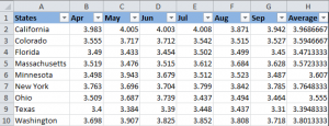
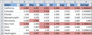
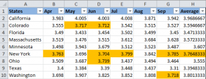
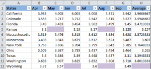
Представим, у вас имеется набор товаров в разных штатах с их ценами, и необходимо знать, какие из них по стоимости превышают 3,7 долларов. Поэтому мы решили те товары, которые находятся выше этого значения, подсвечивать красным цветом. А клетки, имеющие аналогичное или большее значение, решено окрашивать в зеленый оттенок.
Примечание: Скриншот был сделан в программе 2010 версии. Но это не влияет ни на что, поскольку последовательность действий одинаковая, независимо от того, какую версию — последнюю, или нет — использует человек.
Итак, что нужно сделать (пошагово):
1. Выбрать клетки, в которых следует отредактировать оттенок. Например, диапазон $B$2:$H$10 (наименования колонок и первая колонка, в которой приводятся названия штатов, исключены из выборки).
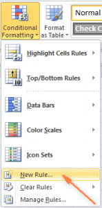
2. Нажать на «Главная» в группе «Стили». Там будет находиться пункт «Условное форматирование». Там же нужно выбрать пункт «Новое правило». В английской версии Excel последовательность шагов следующая: “Home”, “Styles group”, “Conditional Formatting > New Rule».
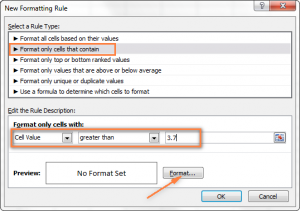
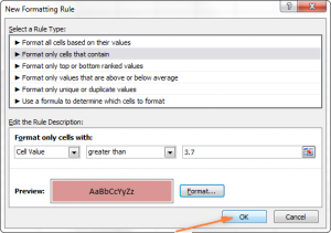
3. В открывшемся окне следует поставить галочку «Форматировать только ячейки, которые содержат» (“Format only cells that contain” в английской версии).
4. Внизу этого окна под надписью «Форматировать только ячейки, для которых выполняется следующее условие» (Format only cells with) можно назначить правила, по которым и будет выполняться форматирование. Мы выбрали формат для указанного значения в клетках, которое должно превышать 3.7, как видно со скриншота:
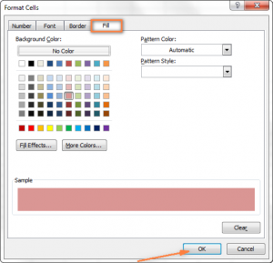
5. Далее следует кликнуть по кнопке «Формат». Появится окно, где слева находится область выбора фонового цвета. Но перед этим следует открыть вкладку “Заполнить” («Fill»). В данном случае это красный оттенок. После этого следует кликнуть по кнопке «ОК».
6. Затем вы возвратитесь в окно «Новое правило форматирования», но уже внизу этого окна можно предварительно посмотреть, как будет выглядеть эта клетка. Если все отлично, нужно нажать на кнопку «ОК».
В результате, получится что-то вроде этого:
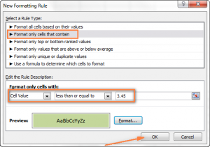
Далее нам необходимо добавить еще одно условие, то есть, поменять фон клеток со значениями меньше 3.45, на зеленый цвет. Для выполнения этой задачи необходимо снова кликнуть на «Новое правило форматирования» и повторить описанные выше шаги, только условие нужно поставить как «меньше чем, или эквивалентно» (в английской версии «less than or equal to», а далее прописать значение. В конце нужно нажать кнопку «ОК».
Теперь таблица отформатирована таким способом.
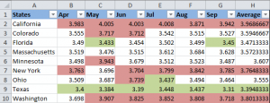
На ней отображаются самые высокие и низкие котировки на топливо в различных штатах, и можно сразу определить, где ситуация наиболее оптимистичная (в Техасе, конечно же).
Рекомендация: Если будет необходимость, можно воспользоваться похожим методом форматирования, редактируя не фон, а шрифт. Для этого в окне форматирования, который появился на пятом этапе, нужно выбрать вкладку «Font» и руководствоваться подсказками, приводимыми в окне. Там все интуитивно понятно, и разобраться может даже новичок.
В результате, получится такая табличка:
Как оставить цвет ячейки таким же, даже если меняется значение?
Задача: Вам необходимо окрасить фон так, чтобы он не менялся никогда, даже если в будущем фон изменится.
Решение: найдите все клетки с определенным числом, используя функцию Excel “Найти все” «Find All» или дополнением “Выбрать особые ячейки” («Select Special Cells»), а после этого отредактировать формат ячейки, пользуясь функцией “Форматировать ячейки” («Format Cells»).
Это одна из тех нечастых ситуаций, которые не предусмотрены в руководстве Excel, и даже в интернете решение этой проблемы можно встретить довольно редко. Что неудивительно, поскольку данная задача не является стандартной. Если необходимо отредактировать фон навсегда, чтобы он никогда не менялся, пока не будет скорректирован пользователем программы вручную, необходимо следовать приведенной выше инструкции.
Выбрать все клетки, которые содержат определенное условие
Существует несколько возможных методов, зависящих от того, какие виды конкретного значения следует найти.
Если надо обозначить особым фоном клетки с определенным значением, необходимо перейти к вкладке «Главная» и выбрать «Найти и выделить” – «Найти».
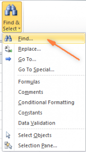
Введите нужные значения и кликните на «Найти все».

Подсказка: Можно кликнуть на кнопку «Параметры» справа, чтобы воспользоваться некоторыми дополнительными настройками: где искать, как просматривать, учитывать ли большие и маленькие буквы, и так далее. Также можно прописывать дополнительные символы, например, звездочку (*), чтобы найти все строки, содержащие эти значения. Если использовать знак вопроса, можно отыскать какой угодно единичный символ.
В нашем прошлом примере, если необходимо найти все котировки на топливо между 3,7 и 3,799 долларов, мы можем уточнить наш поисковой запрос.
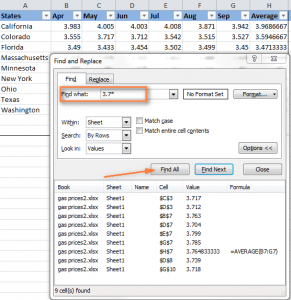
Теперь выберите какое угодно из значений, которые нашла программа, внизу диалогового окна и кликните по одному из них. После этого следует нажать на комбинацию клавиш «Ctrl-A» для выделения всех результатов. Далее нажмите на кнопку «Закрыть».
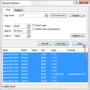
Вот как можно выбрать все клетки с определенными значениями, используя функцию «Найти все». В нашем примере нам необходимо найти все цены на топливо выше 3,7 долларов и, к сожалению, Excel не позволяет делать это с помощью функции «Найти и заменить».
“Бочка меда” здесь обнаруживается благодаря тому, что есть другой инструмент, который поможет в выполнении таких сложных задач. Называется он «Select Special Cells». Это дополнение (которое нужно устанавливать к Excel отдельн), которое поможет:
- найти все значения в определенном диапазоне, например, между -1 и 45,
- получить максимальное или минимальное значение в колонке,
- найти строку или диапазон,
- отыскать клетки по окраске фона и многое другое.
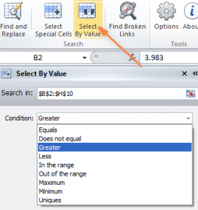
После установки дополнения просто нажмите кнопку “Выбрать по значению” («Select by Value») и потом уточните поисковый запрос в окне аддона. В нашем примере мы ищем числа больше 3,7. Нажмите на “Выбрать” («Select»), и через секунду получите результат наподобие такого:
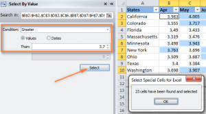
Если дополнение вас заинтересовало, вы можете скачать пробную версию по ссылке.
Изменение фона выбранных клеток через окно «Форматировать ячейки»
Теперь, после того, как все клетки с определенным значением были выделены одним из описанных выше методов, осталось указать цвет фона для них.
Чтобы сделать это, необходимо открыть окно «Формат ячеек», нажав на клавишу Ctrl + 1 (также можно нажать правой кнопкой мышки по выделенным клеткам и кликнуть левой кнопки мыши по пункту «форматирование ячеек») и настроить такое форматирование, которое необходимо.
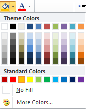
Мы выберем оранжевый оттенок, но можно выбрать любой другой.
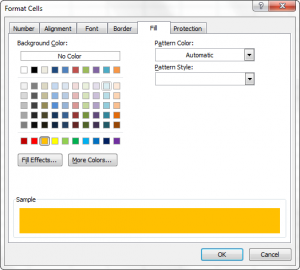
Если надо отредактировать цвет фона, не меняя других параметров внешнего вида, можно просто кликнуть на «заливка цветом» и выбрать цвет, который идеально подходит.
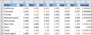
В результате, получится такая таблица:
В отличие от предыдущей техники, здесь цвет клетки не будет изменяться, даже если будет редактироваться значение. Это можно использовать, например, для отслеживания динамики товаров определенной ценовой группы. Их стоимость изменилась, а цвет остался прежним.
Редактирование цвета фона для особенных ячеек (пустых или с ошибками при написании формулы)
Аналогично предыдущему примеру, у пользователя есть возможность редактировать цвет фона специальных клеток двумя способами. Бывает статический и динамический варианты.
Применение формулы для редактирования фона
Здесь окрас ячейки будет редактироваться автоматически, исходя из ее значения. Этот метод во многом помогает пользователям и востребован в 99% ситуаций.
В качестве примера можно использовать прежнюю таблицу, но сейчас часть клеток будет пустой. Нам нужно определить, какие не содержат никаких показаний, и отредактировать цвет фона.
1. На вкладке «Главная» необходимо кликнуть на «Условное форматирование» –> «Новое правило» (так, как в шаге 2 первого раздела «Динамическое изменение цвета фона».
2. Далее необходимо выбрать пункт «Использовать формулу для определения…».
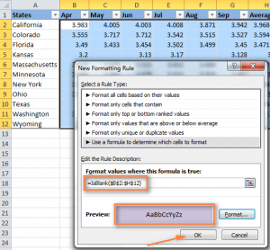
3. Ввести формулу =IsBlank() (ЕПУСТО в русскоязычной версии), если требуется отредактировать фон пустой клетки, или =IsError() (ЕОШИБКА в русскоязычной версии), если надо найти клетку, где есть ошибочно написанная формула. Поскольку в данном случае нам необходимо отредактировать пустые ячейки, вводим формулу =IsBlank(), а потом размещаем курсор между круглыми скобками и нажимаем на кнопку рядом с полем ввода формулы. После этих манипуляций следует выбрать вручную диапазон клеток. Кроме этого, можно указать диапазон самостоятельно, например, =IsBlank(B2:H12).
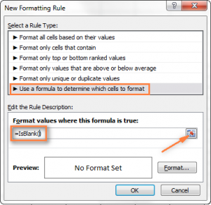
4. Кликнуть по кнопке «Форматировать» и выбрать подходящий фоновый цвет и сделать все так, как описано в пункте 5 раздела «Динамическое изменение цвета фона клетки», а потом нажать «ОК». Там же можно посмотреть, какой будет цвет клетки. Окно будет выглядеть приблизительно так.
5. Если вам понравился фон ячейки, надо нажать на кнопку «ОК», и изменения сразу будут внесены в таблицу.
Статическое изменение фонового цвета специальных ячеек
В данной ситуации единожды назначенный цвет фона продолжит оставаться таким, независимо от того, как клетка будет меняться.
Если необходимо перманентное изменение специальных клеток (пустых или содержащих ошибки), следуйте этой инструкции:
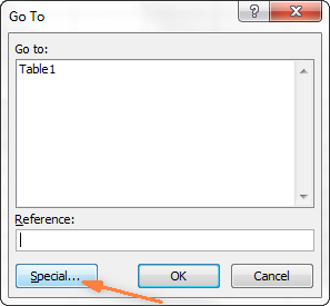
- Выберите ваш документ или несколько ячеек и нажмите на F5 для открытия окна «Переход», а потом нажмите на кнопку «Выделить».

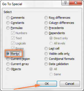
- В открывшемся диалоговом окне выберите кнопку «Blanks» или «Пустые ячейки» (исходя из версии программы — рус. или англ.) для выделения пустых клеток.

- Если вам следует подсветить клетки, имеющие формулы с ошибками, следует выбрать пункт «Формулы» и оставить единственный флажок возле слова «Ошибки». Как следует из скриншота выше, выделять можно клетки по любым параметрам, и каждая из описанных настроек доступна при необходимости.
- Напоследок необходимо изменить цвет фона выделенных ячеек или кастомизировать их любым другим способом. Для этого нужно воспользоваться методом, описанным выше.
Просто помните, что форматирование изменений, выполненное этим способом, будет сохраняться, даже если заполнить пропуски или изменить тип специальной клетки. Конечно, маловероятно, что кто-то захочет применять этот метод, но на практике может быть всякое.
Как выжать максимум из Excel?
Как активные пользователи Microsoft Excel, вы должны знать, что он содержит множество возможностей. Некоторые из них мы знаем и любим, другие же остаются таинственными для среднестатистического пользователя, и большое количество блогеров пытаются пролить хотя бы немного света на них. Но бывают распространенные задачи, которые придется выполнять каждому из нас, а Excel не вводит некоторые возможности или инструменты, чтобы автоматизировать некоторые сложные действия.
И решением этой проблемы становятся дополнения (аддоны). Некоторые из них распространяются бесплатно, другие – за деньги. Существует множество подобных инструментов, которые могут выполнять разные функции. Например, находить дубликаты в двух файлах без загадочных формул или макросов.
Если совмещать эти инструменты с основным функционалом Excel, можно добиться очень больших результатов. Например, можно узнать, какие цены на топливо изменились, а потом обнаружить дубликаты в файле за прошлый год.
Видим, что условное форматирование – это удобный инструмент, который позволяет автоматизировать работу над таблицами без каких-то специфических навыков. Вы теперь умеете несколькими способами заливать клетки, исходя из их содержимого. Теперь осталось только это воплотить на практике. Удачи!
Оцените качество статьи. Нам важно ваше мнение: