
I am using the averageifs function, and have one column where I need to calculate the average if either of the criteria are true.
I have tried using the OR function, and tried the curly brackets, but both give me errors.
=AVERAGEIFS(N1:N612,I1:I612,{«FL»,»IF»})
There are more ranges, but the coding for those is fine.
To be clear, I want to return an average if column «I» contains (specifically) the letters FL, OR the letters IF. Any other letters should mean that entry is not averaged.
TIA!
asked May 27, 2015 at 16:37
![]()
AVERAGEIFS extra criteria is a boolean AND operator, it can’t perform OR operations. But since your columns do not change we can somewhat implement this ourselves:
Here is a simple way using an array formula (entered with ctrl + shift + enter):
=AVERAGE(IF((I1:I612="IF")+(I1:I612="FL"),N1:N612))
Or if you don’t like using array formulas you basically do this manually using SUMPRODUCT and COUNTIF:
=SUMPRODUCT((I1:I612="IF")*(N1:N612)+(I1:I612="FL")*(N1:N612))/(COUNTIF(I1:I612,"IF")+COUNTIF(I1:I612,"FL"))
answered May 27, 2015 at 17:01
![]()
chanceachancea
5,8083 gold badges28 silver badges39 bronze badges
Chancea has given some good techniques I will list one more that avoids array formulas as many will find it easier to read avoiding the sumproduct.
=(SUMIF(I1:I612,"FL",N1:N612)+SUMIF(I1:I612,"IF",N1:N612))/(COUNTIF(I1:I612,"FL")+COUNTIF(I1:I612,"IF"))
answered May 27, 2015 at 18:02
![]()
gtwebbgtwebb
2,9713 gold badges13 silver badges22 bronze badges
1
Do not think Excel has this feature, but in Google Sheets, I’ve been using the below to achieve similar results
=average(filter($A:$A,($C:$C=$E$6)+($C:$C=$E$7)))
giving me an average of the values in A:A where C:C matches the value in either E6 or E7
unlike an ifs / sumifs etc., the filter uses =, not a comma, thus $C:$C=$E$6 is used, not $C:$C,$E$6
Mathematical symbols are just entered ( so <> rather than "<>"& )
![]()
answered Feb 6, 2018 at 14:45
![]()
1
Another way to solve this would be to create an additional column (let’s call it column J) that returns TRUE if column I contains either «FL» or «IF»:
J1 = IF(OR(I1="FL",I1="IF"),TRUE,FALSE)
Then you can reference that column in your AVERAGEIFS formula instead:
=AVERAGEIFS(N1:N612,J1:JI612,TRUE)
answered May 13, 2022 at 23:06
![]()
A solution to your question is:
=AVERAGE(Maxifs(N1:N612,I1:I612,{«FL»;»IF»}))
answered Nov 20, 2022 at 17:04
![]()
Содержание
- AVERAGEIFS function
- Description
- Syntax
- Remarks
- Examples
- AVERAGEIFS Function
- Related functions
- Summary
- Purpose
- Return value
- Arguments
- Syntax
- Usage notes
- Syntax
- Applying criteria
- Multiple criteria
- Value from another cell
- Wildcards
AVERAGEIFS function
This article describes the formula syntax and usage of the AVERAGEIFS function in Microsoft Excel.
Description
Returns the average (arithmetic mean) of all cells that meet multiple criteria.
Syntax
AVERAGEIFS(average_range, criteria_range1, criteria1, [criteria_range2, criteria2], . )
The AVERAGEIFS function syntax has the following arguments:
Average_range Required. One or more cells to average, including numbers or names, arrays, or references that contain numbers.
Criteria_range1, criteria_range2, … Criteria_range1 is required, subsequent criteria_ranges are optional. 1 to 127 ranges in which to evaluate the associated criteria.
Criteria1, criteria2, . Criteria1 is required, subsequent criteria are optional. 1 to 127 criteria in the form of a number, expression, cell reference, or text that define which cells will be averaged. For example, criteria can be expressed as 32, «32», «>32», «apples», or B4.
If average_range is a blank or text value, AVERAGEIFS returns the #DIV0! error value.
If a cell in a criteria range is empty, AVERAGEIFS treats it as a 0 value.
Cells in range that contain TRUE evaluate as 1; cells in range that contain FALSE evaluate as 0 (zero).
Each cell in average_range is used in the average calculation only if all of the corresponding criteria specified are true for that cell.
Unlike the range and criteria arguments in the AVERAGEIF function, in AVERAGEIFS each criteria_range must be the same size and shape as sum_range.
If cells in average_range cannot be translated into numbers, AVERAGEIFS returns the #DIV0! error value.
If there are no cells that meet all the criteria, AVERAGEIFS returns the #DIV/0! error value.
You can use the wildcard characters, question mark (?) and asterisk (*), in criteria. A question mark matches any single character; an asterisk matches any sequence of characters. If you want to find an actual question mark or asterisk, type a tilde (
) before the character.
Note: The AVERAGEIFS function measures central tendency, which is the location of the center of a group of numbers in a statistical distribution. The three most common measures of central tendency are:
Average which is the arithmetic mean, and is calculated by adding a group of numbers and then dividing by the count of those numbers. For example, the average of 2, 3, 3, 5, 7, and 10 is 30 divided by 6, which is 5.
Median which is the middle number of a group of numbers; that is, half the numbers have values that are greater than the median, and half the numbers have values that are less than the median. For example, the median of 2, 3, 3, 5, 7, and 10 is 4.
Mode which is the most frequently occurring number in a group of numbers. For example, the mode of 2, 3, 3, 5, 7, and 10 is 3.
For a symmetrical distribution of a group of numbers, these three measures of central tendency are all the same. For a skewed distribution of a group of numbers, they can be different.
Examples
Copy the example data in the following table, and paste it in cell A1 of a new Excel worksheet. For formulas to show results, select them, press F2, and then press Enter. If you need to, you can adjust the column widths to see all the data.
Источник
AVERAGEIFS Function
Summary
The Excel AVERAGEIFS function calculates the average of numbers in a range that meet one or more criteria. The criteria used for AVERAGEIFS can include logical operators (>, ,=) and wildcards (*,?) for partial matching.
Purpose
Return value
Arguments
- avg_rng — The range to average.
- range1 — The first range to evaulate.
- criteria1 — The criteria to use on range1.
- range2 — [optional] The second range to evaluate.
- criteria2 — [optional] The criteria to use on range2.
Syntax
Usage notes
The AVERAGEIFS function calculates the average of cells in a range that meet one or more conditions, referred to as criteria. To apply criteria, the AVERAGEIFS function supports logical operators (>, ,=) and wildcards (*,?) for partial matching. AVERAGEIFS can be used to average cells based on dates, text values, and numbers.
Syntax
The syntax for the AVERAGEIFS function depends on the criteria being evaluated. Each separate condition will require a range and a criteria. The generic syntax for AVERAGEIFS looks like this:
The first argument, avg_range, is the range of cells to average, which should contain numeric values. The second argument, range1, is the range to which the first condition should be applied. The third argument, criteria1, contains the condition that should be applied to range1, along with any logical operators. Additional conditions are applied by providing additional range/criteria arguments. When using AVERAGEIFS, keep the following in mind:
- Only values that meet all conditions will be included in the final result.
- All ranges must be the same size or AVERAGEIFS will return a #VALUE! error.
- AVERAGEIFS will not include empty cells in the average, even when criteria match.
- AVERAGEIFS will return a #DIV/0! error if no cells meet criteria.
Applying criteria
The AVERAGEIFS function supports logical operators (>, ,=) and wildcards (*,?) for partial matching. Because AVERAGEIFS is in a group of eight functions that split logical criteria into two parts, the syntax is a bit tricky. Each condition requires a separate range and criteria, and operators need to be enclosed in double quotes («»). The table below shows some common examples:
| Target | Criteria |
|---|---|
| Cells greater than 75 | «>75» |
| Cells equal to 100 | 100 or «100» |
| Cells less than or equal to 100 | » red» |
| Cells that are blank «» | «» |
| Cells that are not blank | «<>« |
| Cells that begin with «X» | «x*» |
| Cells less than A1 | » =), the operator and number are both enclosed in double quotes.
Double quotes are also used for text values. For example, to average values in B1:B10 when values in A1:A10 equal «red», you can use a formula like this: Multiple criteriaEnter criteria in pairs [range, criteria]. For example, to average values in A1:A10, where B1:B10 = «A», and C1:C10 > 5, use: Value from another cellA value from another cell can be included in criteria using concatenation. In the example below, AVERAGEIFS will return the average of numbers in A1:A10 that are less than the value in cell B1. Notice the less than operator (which is text) is enclosed in quotes. WildcardsThe wildcard characters question mark (?), asterisk(*), or tilde ( ) can be used in criteria. A question mark (?) matches any one character and an asterisk (*) matches zero or more characters of any kind. For example, to average values in B1:B10 when values in A1:A10 contain the text «red», you can use a formula like this: ) is an escape character to allow you to find literal wildcards. For example, to match a literal question mark (?), asterisk(*), or tilde ( ), add a tilde in front of the wildcard (i.e. Note: the order of arguments is different between AVERAGEIFS and AVERAGEIF. The range to average is always the first argument in AVERAGEIFS. Источник Adblock |
This article describes the formula syntax and usage of the AVERAGEIFS function in Microsoft Excel.
Description
Returns the average (arithmetic mean) of all cells that meet multiple criteria.
Syntax
AVERAGEIFS(average_range, criteria_range1, criteria1, [criteria_range2, criteria2], …)
The AVERAGEIFS function syntax has the following arguments:
-
Average_range Required. One or more cells to average, including numbers or names, arrays, or references that contain numbers.
-
Criteria_range1, criteria_range2, … Criteria_range1 is required, subsequent criteria_ranges are optional. 1 to 127 ranges in which to evaluate the associated criteria.
-
Criteria1, criteria2, … Criteria1 is required, subsequent criteria are optional. 1 to 127 criteria in the form of a number, expression, cell reference, or text that define which cells will be averaged. For example, criteria can be expressed as 32, «32», «>32», «apples», or B4.
Remarks
-
If average_range is a blank or text value, AVERAGEIFS returns the #DIV0! error value.
-
If a cell in a criteria range is empty, AVERAGEIFS treats it as a 0 value.
-
Cells in range that contain TRUE evaluate as 1; cells in range that contain FALSE evaluate as 0 (zero).
-
Each cell in average_range is used in the average calculation only if all of the corresponding criteria specified are true for that cell.
-
Unlike the range and criteria arguments in the AVERAGEIF function, in AVERAGEIFS each criteria_range must be the same size and shape as sum_range.
-
If cells in average_range cannot be translated into numbers, AVERAGEIFS returns the #DIV0! error value.
-
If there are no cells that meet all the criteria, AVERAGEIFS returns the #DIV/0! error value.
-
You can use the wildcard characters, question mark (?) and asterisk (*), in criteria. A question mark matches any single character; an asterisk matches any sequence of characters. If you want to find an actual question mark or asterisk, type a tilde (~) before the character.
Note: The AVERAGEIFS function measures central tendency, which is the location of the center of a group of numbers in a statistical distribution. The three most common measures of central tendency are:
-
Average which is the arithmetic mean, and is calculated by adding a group of numbers and then dividing by the count of those numbers. For example, the average of 2, 3, 3, 5, 7, and 10 is 30 divided by 6, which is 5.
-
Median which is the middle number of a group of numbers; that is, half the numbers have values that are greater than the median, and half the numbers have values that are less than the median. For example, the median of 2, 3, 3, 5, 7, and 10 is 4.
-
Mode which is the most frequently occurring number in a group of numbers. For example, the mode of 2, 3, 3, 5, 7, and 10 is 3.
For a symmetrical distribution of a group of numbers, these three measures of central tendency are all the same. For a skewed distribution of a group of numbers, they can be different.
Examples
Copy the example data in the following table, and paste it in cell A1 of a new Excel worksheet. For formulas to show results, select them, press F2, and then press Enter. If you need to, you can adjust the column widths to see all the data.
|
Student |
First |
Second |
Final |
|---|---|---|---|
|
Quiz |
Quiz |
Exam |
|
|
Grade |
Grade |
Grade |
|
|
Emilio |
75 |
85 |
87 |
|
Julie |
94 |
80 |
88 |
|
Hans |
86 |
93 |
Incomplete |
|
Frederique |
Incomplete |
75 |
75 |
|
Formula |
Description |
Result |
|
|
=AVERAGEIFS(B2:B5, B2:B5, «>70», B2:B5, «<90») |
Average first quiz grade that falls between 70 and 90 for all students (80.5). The score marked «Incomplete» is not included in the calculation because it is not a numerical value. |
75 |
|
|
=AVERAGEIFS(C2:C5, C2:C5, «>95») |
Average second quiz grade that is greater than 95 for all students. Because there are no scores greater than 95, #DIV0! is returned. |
#DIV/0! |
|
|
=AVERAGEIFS(D2:D5, D2:D5, «<>Incomplete», D2:D5, «>80») |
Average final exam grade that is greater than 80 for all students (87.5). The score marked «Incomplete» is not included in the calculation because it is not a numerical value. |
87.5 |
Example 2
|
Type |
Price |
Town |
Number of Bedrooms |
Garage? |
|---|---|---|---|---|
|
Cozy Rambler |
230000 |
Issaquah |
3 |
No |
|
Snug Bungalow |
197000 |
Bellevue |
2 |
Yes |
|
Cool Cape Codder |
345678 |
Bellevue |
4 |
Yes |
|
Splendid Split Level |
321900 |
Issaquah |
2 |
Yes |
|
Exclusive Tudor |
450000 |
Bellevue |
5 |
Yes |
|
Classy Colonial |
395000 |
Bellevue |
4 |
No |
|
Formula |
Description |
Result |
||
|
=AVERAGEIFS(B2:B7, C2:C7, «Bellevue», D2:D7, «>2»,E2:E7, «Yes») |
Average price of a home in Bellevue that has at least 3 bedrooms and a garage |
397839 |
||
|
=AVERAGEIFS(B2:B7, C2:C7, «Issaquah», D2:D7, «<=3»,E2:E7, «No») |
Average price of a home in Issaquah that has up to 3 bedrooms and no garage |
230000 |
I’ve got a series of blood pressure measurements. I want to determine the average pressures during the day and during the night.

The first half of the problem is trivial:
=AVERAGEIFS(B17:B71;A17:A71;">="&I16;A17:A71;"<="&I17)
builds the average over all cells in column B («Sys») if the corresponding value of column A («Time») is greater than 7:00 and less than 22:00 (those time values are in cells I16/17).
My problem is how to calculate the average for the hours outside that range. I would have to check if the time is smaller than 7:00 or greater than 22:00, but AVERAGEIFS conditions are combined by AND.
I obviously can’t use NOT() because I would have to apply it to the result of both comparisons at once, and there doesn’t seem to be a way to do that.
Conditional highlighting is not a problem as you can see above — there I can enter several conditions that are tested sequentially, effectively giving me an OR operator…
Is there maybe a function I can use to get a subset of cells from a range that I can apply another function to? I’ll probably need something like that anyway when I want to determined blood pressure maxima and minima for day/night — Excel doesn’t have a MAXIFS() function…
The AVERAGEIFS function calculates the average of cells in a range that meet one or more conditions, referred to as criteria. To apply criteria, the AVERAGEIFS function supports logical operators (>,<,<>,=) and wildcards (*,?) for partial matching. AVERAGEIFS can be used to average cells based on dates, text values, and numbers.
Syntax
The syntax for the AVERAGEIFS function depends on the criteria being evaluated. Each separate condition will require a range and a criteria. The generic syntax for AVERAGEIFS looks like this:
=AVERAGEIFS(avg_range,range1,criteria1) // 1 condition
=AVERAGEIFS(avg_range,range1,criteria1,range2,criteria2) // 2 conditions
The first argument, avg_range, is the range of cells to average, which should contain numeric values. The second argument, range1, is the range to which the first condition should be applied. The third argument, criteria1, contains the condition that should be applied to range1, along with any logical operators. Additional conditions are applied by providing additional range/criteria arguments. When using AVERAGEIFS, keep the following in mind:
- Only values that meet all conditions will be included in the final result.
- All ranges must be the same size or AVERAGEIFS will return a #VALUE! error.
- AVERAGEIFS will not include empty cells in the average, even when criteria match.
- AVERAGEIFS will return a #DIV/0! error if no cells meet criteria.
Applying criteria
The AVERAGEIFS function supports logical operators (>,<,<>,=) and wildcards (*,?) for partial matching. Because AVERAGEIFS is in a group of eight functions that split logical criteria into two parts, the syntax is a bit tricky. Each condition requires a separate range and criteria, and operators need to be enclosed in double quotes («»). The table below shows some common examples:
| Target | Criteria |
|---|---|
| Cells greater than 75 | «>75» |
| Cells equal to 100 | 100 or «100» |
| Cells less than or equal to 100 | «<=100» |
| Cells equal to «Red» | «red» |
| Cells not equal to «Red» | «<>red» |
| Cells that are blank «» | «» |
| Cells that are not blank | «<>» |
| Cells that begin with «X» | «x*» |
| Cells less than A1 | «<«&A1 |
| Cells less than today | «<«&TODAY() |
Notice the last two examples use concatenation with the ampersand (&) character. When a criteria argument includes a value from another cell, or the result of a formula, logical operators like «<» must be joined with concatenation. This is because Excel needs to evaluate cell references and formulas first in order to get a value, before that value can be joined with an operator.
Examples
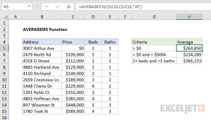
In the example shown, the formulas in H5:H7 are:
=AVERAGEIFS(C5:C15,C5:C15,">0")
=AVERAGEIFS(C5:C15,C5:C15,">0",C5:C15,"<500000")
=AVERAGEIFS(C5:C15,D5:D15,">=2",E5:E15,">1")
These formulas return the average price of properties where:
- prices are greater than zero
- prices are greater than zero and less than $500,000
- properties have at least 2 bedrooms and more than 1 bathroom
Double quotes («») in criteria
In general, text values in criteria are enclosed in double quotes («»), and numbers are not. However, when a logical operator is included with a number, the number and operator must be enclosed in quotes. Note the difference in the two examples below. Because the second formula uses the greater than or equal to operator (>=), the operator and number are both enclosed in double quotes.
=AVERAGEIFS(C5:C15,D5:D15,2) // 2 bedrooms
=AVERAGEIFS(C5:C15,D5:D15,">=2") // 2+ bedrooms
Double quotes are also used for text values. For example, to average values in B1:B10 when values in A1:A10 equal «red», you can use a formula like this:
=AVERAGEIFS(B1:B10,A1:A10,"red")
Multiple criteria
Enter criteria in pairs [range, criteria]. For example, to average values in A1:A10, where B1:B10 = «A», and C1:C10 > 5, use:
=AVERAGEIFS(A1:A10,B1:B10,"A",C1:C10,">5")
Value from another cell
A value from another cell can be included in criteria using concatenation. In the example below, AVERAGEIFS will return the average of numbers in A1:A10 that are less than the value in cell B1. Notice the less than operator (which is text) is enclosed in quotes.
=AVERAGEIFS(A1:A10,A1:A10,"<"&B1) // average values less than B1
Wildcards
The wildcard characters question mark (?), asterisk(*), or tilde (~) can be used in criteria. A question mark (?) matches any one character and an asterisk (*) matches zero or more characters of any kind. For example, to average values in B1:B10 when values in A1:A10 contain the text «red», you can use a formula like this:
=AVERAGEIFS(B1:B10,A1:A10,"*red*")
The tilde (~) is an escape character to allow you to find literal wildcards. For example, to match a literal question mark (?), asterisk(*), or tilde (~), add a tilde in front of the wildcard (i.e. ~?, ~*, ~~).
Note: the order of arguments is different between AVERAGEIFS and AVERAGEIF. The range to average is always the first argument in AVERAGEIFS.
Notes
- All ranges must be the same size or AVERAGEIFS will return a #VALUE! error.
- Only values that meet all conditions will be included in the final result.
- AVERAGEIFS will not include empty cells in the average, even when criteria match.
- TRUE and FALSE values ignored when calculating an average.
- AVERAGEIFS will return a #DIV/0! error if no cells meet criteria.
- AVERAGEIFS requires a range, you can’t substitute an array.
- Logical operators and text values should be enclosed in double quotes («»).
- AVERAGEIFS supports wildcards but is not case-sensitive.