
AVERAGEIF and AVERAGEIFS are both Statistical functions n Microsoft Excel. In this post, we will take a look at their syntax and how to use them.
The AVERAGEIF function evaluates the average of all numbers in a range that meet a given criterion. The formula for the AVERAGEIF is:
Averageif (Range, criteria, [average_range])
The AVERAGEIFS function returns the average of all numbers in a range that meets multiple criteria. The formula for AVERAGEIFS is:
Averageifs (average_range, criteria_range1, criteria1[criteria_ range2, criteria2] …)
Syntax of AVERAGEIF and AVERAGEIFS
AVERAGEIF
- Range: is the group of cells you want to average. The Range is required.
- Criteria: The Criteria is used to verify which cells to average. Criteria are required.
- Average_range: The Range of cells to average. When absent, the range parameter will be average instead. Average_range is optional.
AVERAGEIFS
- Average_range: The Average_ Range is one or more cells to average. Average_range is required.
- Range: the group of cells you want to average. The Range is required.
- Criteria_range1: The first Range to evaluate the related criteria. The first Criteria_range1 is required, but the second criteria_ range is optional.
- Criteria 1: The Criteria verify which cells to average. The first criteria are required. The second criteria or any criteria after is optional.
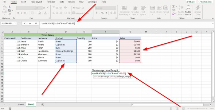
First, we are going to click the cell where we want the Average. Then type =Averageif bracket.
Inside the bracket, we will type the Range because the Range of cells contains the data we want to average.
In this tutorial, we will type the cell (D3:D9), or we can click on the cell in the column that we want to average and drag it to the end; this will automatically place the range of cells in the formula.
Now, we are going to enter the Criteria; the criteria validate which cells to average. We are going to use Bread in this tutorial because it is what we are looking for.
We are going to enter the Average_ range. We will type G3:G9 because these cells contain the sales we want to average; then close the bracket.
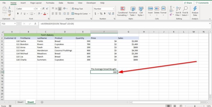
Press Enter, you will see the result.
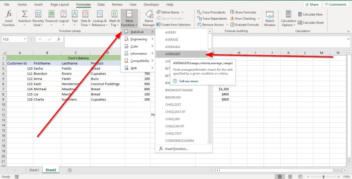
The other option is to go to Formulas. In the Function Library group, select More Functions. In the drop-down menu list, select Statistical in its menu choose AVERAGEIF. A Function Argument dialog box will appear.
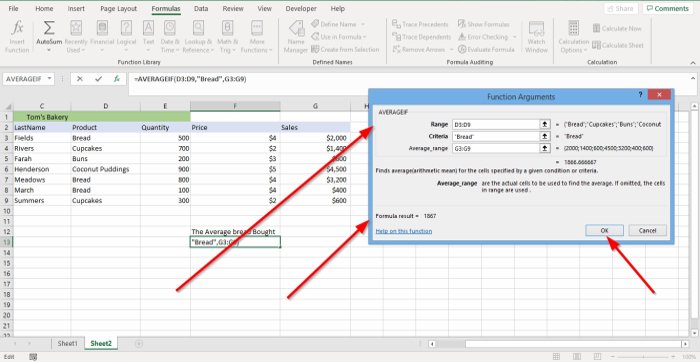
In the Function Arguments dialog box, where you see Range, type D3:D9 into its entry box.
In the Function Arguments dialog box, where you see Criteria, type “Bread” into the criteria entry box.
In the Function Arguments dialog box, where you see Average_range, type G3:G9 into its entry box.
Click OK and you will see your result.
Read: How to use SUMIF and SUMIFS Functions in Excel
How to use AVERAGEIFS in Excel
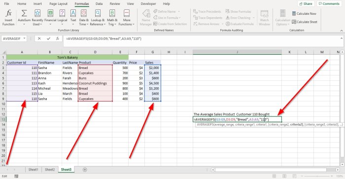
In this tutorial, we are going to look up the average sale of products bought by customer 110.
Click the cell where you want the result in, then type =Averageif, bracket.
In the bracket type G3:G9, this is the Average_range.
Now we are going to type the Criteria_range1. Type D3:D9, this range of cells contain the data we are looking for.
We will type the Criteria1, which is” Bread” because it is the product we are looking for.
We are going to fine Criteria_range2, which is A3:A9 because we want to identify the customer.
We will enter Criteria2, which is“110,” because this is the ID number of the customer we are looking for.

Press Enter and you will see your result.
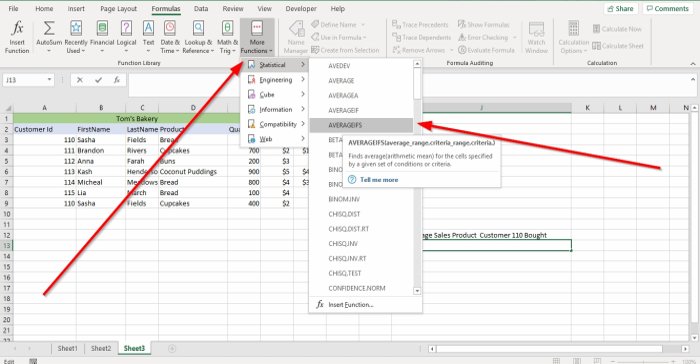
The other option is to go to Formulas. In the Function Library group, select More Functions. In the drop-down menu list, select Statistical in its menu select AVERAGEIFS; and a Function Argument dialog box will appear.

In the Function Arguments dialog box, where you see Average_range. Type G3:G9 in its entry box.
In the Function Arguments dialog box, where you see Criteria_range1. Type D3:D9 in its entry box.
In the Criteria1 entry box, type Bread.
In the Criteria_range2 entry box, type A3:A9.
In the Criteria2 entry box, type “110” because we are looking for the customer id 110.
Click OK. You will see the result.
Read next: How to use the IF Function in Excel.
This article describes the formula syntax and usage of the AVERAGEIFS function in Microsoft Excel.
Description
Returns the average (arithmetic mean) of all cells that meet multiple criteria.
Syntax
AVERAGEIFS(average_range, criteria_range1, criteria1, [criteria_range2, criteria2], …)
The AVERAGEIFS function syntax has the following arguments:
-
Average_range Required. One or more cells to average, including numbers or names, arrays, or references that contain numbers.
-
Criteria_range1, criteria_range2, … Criteria_range1 is required, subsequent criteria_ranges are optional. 1 to 127 ranges in which to evaluate the associated criteria.
-
Criteria1, criteria2, … Criteria1 is required, subsequent criteria are optional. 1 to 127 criteria in the form of a number, expression, cell reference, or text that define which cells will be averaged. For example, criteria can be expressed as 32, «32», «>32», «apples», or B4.
Remarks
-
If average_range is a blank or text value, AVERAGEIFS returns the #DIV0! error value.
-
If a cell in a criteria range is empty, AVERAGEIFS treats it as a 0 value.
-
Cells in range that contain TRUE evaluate as 1; cells in range that contain FALSE evaluate as 0 (zero).
-
Each cell in average_range is used in the average calculation only if all of the corresponding criteria specified are true for that cell.
-
Unlike the range and criteria arguments in the AVERAGEIF function, in AVERAGEIFS each criteria_range must be the same size and shape as sum_range.
-
If cells in average_range cannot be translated into numbers, AVERAGEIFS returns the #DIV0! error value.
-
If there are no cells that meet all the criteria, AVERAGEIFS returns the #DIV/0! error value.
-
You can use the wildcard characters, question mark (?) and asterisk (*), in criteria. A question mark matches any single character; an asterisk matches any sequence of characters. If you want to find an actual question mark or asterisk, type a tilde (~) before the character.
Note: The AVERAGEIFS function measures central tendency, which is the location of the center of a group of numbers in a statistical distribution. The three most common measures of central tendency are:
-
Average which is the arithmetic mean, and is calculated by adding a group of numbers and then dividing by the count of those numbers. For example, the average of 2, 3, 3, 5, 7, and 10 is 30 divided by 6, which is 5.
-
Median which is the middle number of a group of numbers; that is, half the numbers have values that are greater than the median, and half the numbers have values that are less than the median. For example, the median of 2, 3, 3, 5, 7, and 10 is 4.
-
Mode which is the most frequently occurring number in a group of numbers. For example, the mode of 2, 3, 3, 5, 7, and 10 is 3.
For a symmetrical distribution of a group of numbers, these three measures of central tendency are all the same. For a skewed distribution of a group of numbers, they can be different.
Examples
Copy the example data in the following table, and paste it in cell A1 of a new Excel worksheet. For formulas to show results, select them, press F2, and then press Enter. If you need to, you can adjust the column widths to see all the data.
|
Student |
First |
Second |
Final |
|---|---|---|---|
|
Quiz |
Quiz |
Exam |
|
|
Grade |
Grade |
Grade |
|
|
Emilio |
75 |
85 |
87 |
|
Julie |
94 |
80 |
88 |
|
Hans |
86 |
93 |
Incomplete |
|
Frederique |
Incomplete |
75 |
75 |
|
Formula |
Description |
Result |
|
|
=AVERAGEIFS(B2:B5, B2:B5, «>70», B2:B5, «<90») |
Average first quiz grade that falls between 70 and 90 for all students (80.5). The score marked «Incomplete» is not included in the calculation because it is not a numerical value. |
75 |
|
|
=AVERAGEIFS(C2:C5, C2:C5, «>95») |
Average second quiz grade that is greater than 95 for all students. Because there are no scores greater than 95, #DIV0! is returned. |
#DIV/0! |
|
|
=AVERAGEIFS(D2:D5, D2:D5, «<>Incomplete», D2:D5, «>80») |
Average final exam grade that is greater than 80 for all students (87.5). The score marked «Incomplete» is not included in the calculation because it is not a numerical value. |
87.5 |
Example 2
|
Type |
Price |
Town |
Number of Bedrooms |
Garage? |
|---|---|---|---|---|
|
Cozy Rambler |
230000 |
Issaquah |
3 |
No |
|
Snug Bungalow |
197000 |
Bellevue |
2 |
Yes |
|
Cool Cape Codder |
345678 |
Bellevue |
4 |
Yes |
|
Splendid Split Level |
321900 |
Issaquah |
2 |
Yes |
|
Exclusive Tudor |
450000 |
Bellevue |
5 |
Yes |
|
Classy Colonial |
395000 |
Bellevue |
4 |
No |
|
Formula |
Description |
Result |
||
|
=AVERAGEIFS(B2:B7, C2:C7, «Bellevue», D2:D7, «>2»,E2:E7, «Yes») |
Average price of a home in Bellevue that has at least 3 bedrooms and a garage |
397839 |
||
|
=AVERAGEIFS(B2:B7, C2:C7, «Issaquah», D2:D7, «<=3»,E2:E7, «No») |
Average price of a home in Issaquah that has up to 3 bedrooms and no garage |
230000 |
На чтение 2 мин
Функция СРЗНАЧЕСЛИМН (AVERAGEIFS) в Excel используется для вычисления среднего арифметического значения по заданному диапазону и нескольким критериям.
Содержание
- Что возвращает функция
- Синтаксис
- Аргументы функции
- Дополнительная информация
- Примеры использования функции СРЗНАЧЕСЛИМН в Excel
Что возвращает функция
Возвращает число, обозначающее среднее арифметическое по заданному диапазону ячеек, отвечающих заданным нескольким критериям.
 Больше лайфхаков в нашем Telegram Подписаться
Синтаксис
=AVERAGEIFS(average_range, criteria_range1, criteria1, [criteria_range2, criteria2], …) — английская версия
=СРЗНАЧЕСЛИМН(диапазон_усреднения;диапазон_условий1;условие1;[диапазон_условий2;условие2];…) — русская версия
Аргументы функции
- average_range (диапазон_усреднения) — диапазон ячеек, по которому будет осуществлена проверка на соответствие заданному критерию;
- criteria_range1, criteria_range2,.. (диапазон_условий) — диапазон ячеек, по которому с помощью заданного критерия функция определит, для каких ячеек требуется провести вычисление среднего арифметического;
- criteria1, criteria 2,..(условие) — критерий, по которому функция определяет, для каких ячеек требуется проводить вычисления.
Дополнительная информация
- если в диапазоне ячеек атрибута average_range есть текстовые значения или пустые ячейки, функция выдаст ошибку;
- критерием могут быть числа, выражения, ссылка на ячейку, текст или формула;
- критерий указанный в качестве текста, математического или логического символа (=,+,-,/,*) должны быть указаны в двойных кавычках;
- в качестве критерия могут использоваться подстановочные знаки;
вычисление среднего арифметического по атрибуту функции average_range (диапазон_усреднения) вычисляются только при соблюдении всех выше описанных требований; - размер диапазона атрибута average_range (диапазон_усреднения) и criteria_range (диапазон_условий) должны быть равны;
Примеры использования функции СРЗНАЧЕСЛИМН в Excel
Содержание
- Обзор функции СРЗНАЧЕСЛИ
- Синтаксис и аргументы функции СРЗНАЧЕСЛИ:
- Что такое функция СРЗНАЧЕСЛИ?
- AVERAGEIF в Google Таблицах
В этом руководстве показано, как использовать функции Excel AVERAGEIF и AVERAGEIFS в Excel и Google Sheets для усреднения данных, соответствующих определенным критериям.

Обзор функции СРЗНАЧЕСЛИ
Вы можете использовать функцию СРЗНАЧЕСЛИ в Excel для подсчета ячеек, содержащих определенное значение, подсчета ячеек, которые больше или равны значению и т. Д.
Чтобы использовать функцию рабочего листа Excel СРЗНАЧЕСЛИ, выберите ячейку и введите:

(Обратите внимание, как появляются входные данные формулы)
Синтаксис и аргументы функции СРЗНАЧЕСЛИ:
= СРЗНАЧЕСЛИ (диапазон; критерии; [средний_ диапазон])
диапазон — Диапазон подсчитываемых ячеек.
критерии — Критерии, определяющие, какие ячейки следует подсчитывать.
средний_ диапазон — [необязательно] Ячейки для усреднения. Если не указано, используется диапазон.
Что такое функция СРЗНАЧЕСЛИ?
Функция СРЗНАЧЕСЛИ — одна из старых функций, используемых в электронных таблицах. Он используется для сканирования диапазона ячеек, проверяя определенный критерий, а затем выдает среднее значение (также называемое математическим средним) для значений в диапазоне, которые соответствуют этим значениям. Исходная функция СРЗНАЧЕСЛИ ограничивалась только одним критерием. После 2007 года была создана функция СРЗНАЧЕСЛИМН, которая позволяет использовать множество критериев. В основном они используются одинаково, но есть некоторые важные различия в синтаксисе, которые мы обсудим в этой статье.
Если вы еще этого не сделали, вы можете просмотреть большую часть аналогичной структуры и примеры в статье СЧЁТЕСЛИМН.
Базовый пример
Давайте рассмотрим этот список зарегистрированных продаж, и мы хотим знать средний доход.

Поскольку у нас были расходы, отрицательное значение, мы не можем просто вычислить базовое среднее значение. Вместо этого мы хотим усреднить только те значения, которые больше 0. «Больше 0» — это то, что будет нашим критерием в функции СРЗНАЧЕСЛИ. Наша формула для утверждения, что это
= СРЗНАЧЕСЛИ (A2: A7; "> 0")

Пример с двумя столбцами
Хотя исходная функция СРЗНАЧЕСЛИ была разработана, чтобы позволить вам применить критерий к диапазону чисел, которые вы хотите суммировать, большую часть времени вам потребуется применить один или несколько критериев к другим столбцам. Рассмотрим эту таблицу:

Теперь, если мы воспользуемся исходной функцией СРЗНАЧЕСЛИ, чтобы узнать, сколько бананов у нас в среднем. Мы поместим наши критерии в ячейку D1, и нам нужно будет указать диапазон, который мы хотим в среднем в качестве последнего аргумента, и поэтому наша формула будет
= СРЗНАЧЕСЛИ (A2: A7; D1; B2: B7)

Однако, когда программисты в конце концов поняли, что пользователи хотят давать более одного критерия, была создана функция СРЗНАЧЕСЛИМН. Чтобы создать одну структуру, которая будет работать для любого количества критериев, для СРЕДНЕЛИН необходимо, чтобы диапазон сумм был указан первым. В нашем примере это означает, что формула должна быть
= СРЕДНЕЛИН (B2: B7; A2: A7; D1)

ПРИМЕЧАНИЕ. Эти две формулы дают одинаковый результат и могут выглядеть примерно одинаково, поэтому обратите особое внимание на то, какая функция используется, чтобы убедиться, что вы перечислили все аргументы в правильном порядке.
Работа с датами, несколько критериев
При работе с датами в электронной таблице, хотя можно ввести дату непосредственно в формулу, лучше всего иметь дату в ячейке, чтобы вы могли просто ссылаться на ячейку в формуле. Например, это помогает компьютеру понять, что вы хотите использовать дату 27.05.2020, а не число 5, разделенное на 27, разделенное на 2022 год.
Давайте посмотрим на нашу следующую таблицу, в которой регистрируется количество посетителей сайта каждые две недели.

Мы можем указать начальную и конечную точки диапазона, который мы хотим посмотреть в D2 и E2. Наша формула для определения среднего числа посетителей в этом диапазоне может быть:
= AVERAGEIFS (B2: B7, A2: A7, "> =" & D2, A2: A7, "<=" & E2)

Обратите внимание, как мы смогли объединить сравнения «=» со ссылками на ячейки для создания критериев. Кроме того, хотя оба критерия применялись к одному и тому же диапазону ячеек (A2: A7), вам необходимо записать диапазон дважды, по одному разу для каждого критерия.
Несколько столбцов
При использовании нескольких критериев вы можете применить их к тому же диапазону, что и в предыдущем примере, или вы можете применить их к разным диапазонам. Давайте объединим наши образцы данных в эту таблицу:

Мы настроили несколько ячеек, чтобы пользователь мог вводить то, что он хочет искать, в ячейках с E2 по G2. Таким образом, нам нужна формула, которая суммирует общее количество яблок, собранных в феврале. Наша формула выглядит так:
= AVERAGEIFS (C2: C7, B2: B7, "> =" & F2, B2: B7, "<=" & G2, A2: A7, E2)

AVERAGEIFS с логикой типа ИЛИ
До этого момента все примеры, которые мы использовали, основывались на сравнении на основе И, когда мы ищем строки, соответствующие всем нашим критериям. Теперь рассмотрим случай, когда вы хотите найти возможность строки, соответствующей тому или иному критерию.
Давайте посмотрим на этот список продаж:

Мы хотели бы сложить средние продажи для Адама и Боба. Во-первых, быстрое обсуждение усреднения. Если у вас нечетное количество вещей, например 3 записи для Адама и 2 для Боба, вы не можете просто взять среднее значение продаж каждого человека. Это называется усреднением средних значений, и в итоге вы придаете несправедливый вес элементу, в котором мало записей. Если это так с вашими данными, вам нужно будет вычислить среднее значение «вручную»: возьмите сумму всех ваших товаров, разделенную на количество ваших товаров. Чтобы узнать, как это сделать, вы можете ознакомиться со статьями здесь:
Теперь, если количество записей такое же, как в нашей таблице, у вас есть несколько вариантов, которые вы можете сделать. Самый простой — сложить два СРЗНАЧЕСЛИМН вместе, вот так, а затем разделить на 2 (количество элементов в нашем списке).
= (СРЕДНЕНОМН (B2: B7; A2: A7; «Адам») + СРЕДНЕМН (B2: B7; A2: A7; «Боб»)) / 2

Здесь компьютер подсчитывает наши индивидуальные баллы, а затем мы складываем их.
Наш следующий вариант подходит, когда у вас больше диапазонов критериев, так что вам не нужно повторно переписывать всю формулу. В предыдущей формуле мы вручную приказали компьютеру сложить два разных СРЕДНЕГО РАЗМНЕНИЯ. Однако вы также можете сделать это, записав свои критерии внутри массива, например:
= СРЕДНИЙ (СРЕДНЕЛИ (B2: B7; A2: A7; {"Адам"; "Боб"}))

Посмотрите, как построен массив в фигурных скобках. Когда компьютер вычисляет эту формулу, он будет знать, что мы хотим вычислить функцию СРЗНАЧЕСЛИМН для каждого элемента в нашем массиве, создав таким образом массив чисел. Затем внешняя функция AVERAGE возьмет этот массив чисел и превратит его в одно число. Пошаговая оценка формулы будет выглядеть так:
= СРЕДНИЙ (СРЕДНИЙ (B2: B7, A2: A7, {"Адам", "Боб"})) = СРЕДНИЙ (13701, 21735) = 17718
Получаем тот же результат, но формулу удалось записать более лаконично.
Работа с пробелами
Иногда в вашем наборе данных есть пустые ячейки, которые вам нужно либо найти, либо избежать. Настройка критериев для них может быть немного сложной, поэтому давайте рассмотрим другой пример.

Обратите внимание, что ячейка A3 действительно пуста, а в ячейке A5 есть формула, возвращающая строку нулевой длины «». Если мы хотим найти общее среднее значение действительно пустые ячейки, мы использовали бы критерий «=», и наша формула выглядела бы так:
= СРЗНАЧЕСЛИМН (B2: B7; A2: A7; "=")

С другой стороны, если мы хотим получить среднее значение для всех ячеек, которые визуально выглядят пустыми, мы изменим критерий на «», и формула будет выглядеть так:
= СРЗНАЧЕСЛИМН (B2: B7; A2: A7; "")

Давайте перевернем: что, если вы хотите найти среднее значение непустых ячеек? К сожалению, текущий дизайн не позволяет избежать строки нулевой длины. Вы можете использовать критерий «», но, как вы можете видеть в примере, он по-прежнему включает значение из строки 5.
= СРЗНАЧЕСЛИМН (B2: B7; A2: A7; "")

Если вам нужно не подсчитывать ячейки, содержащие строки нулевой длины, вы можете рассмотреть возможность использования функции LEN внутри СУММПРОИЗВ.
AVERAGEIF в Google Таблицах
Функция СРЗНАЧЕСЛИ работает в Google Таблицах точно так же, как и в Excel:

Содержание
- AVERAGEIFS function
- Description
- Syntax
- Remarks
- Examples
- AVERAGEIFS function
- Description
- Syntax
- Remarks
- Examples
- AVERAGEIF function
- Description
- Syntax
- Remarks
- Examples
- Метод WorksheetFunction.AverageIfs (Excel)
- Синтаксис
- Параметры
- Возвращаемое значение
- Замечания
- Поддержка и обратная связь
- AVERAGEIFS function
- Description
- Syntax
- Remarks
- Examples
AVERAGEIFS function
This article describes the formula syntax and usage of the AVERAGEIFS function in Microsoft Excel.
Description
Returns the average (arithmetic mean) of all cells that meet multiple criteria.
Syntax
AVERAGEIFS(average_range, criteria_range1, criteria1, [criteria_range2, criteria2], . )
The AVERAGEIFS function syntax has the following arguments:
Average_range Required. One or more cells to average, including numbers or names, arrays, or references that contain numbers.
Criteria_range1, criteria_range2, … Criteria_range1 is required, subsequent criteria_ranges are optional. 1 to 127 ranges in which to evaluate the associated criteria.
Criteria1, criteria2, . Criteria1 is required, subsequent criteria are optional. 1 to 127 criteria in the form of a number, expression, cell reference, or text that define which cells will be averaged. For example, criteria can be expressed as 32, «32», «>32», «apples», or B4.
If average_range is a blank or text value, AVERAGEIFS returns the #DIV0! error value.
If a cell in a criteria range is empty, AVERAGEIFS treats it as a 0 value.
Cells in range that contain TRUE evaluate as 1; cells in range that contain FALSE evaluate as 0 (zero).
Each cell in average_range is used in the average calculation only if all of the corresponding criteria specified are true for that cell.
Unlike the range and criteria arguments in the AVERAGEIF function, in AVERAGEIFS each criteria_range must be the same size and shape as sum_range.
If cells in average_range cannot be translated into numbers, AVERAGEIFS returns the #DIV0! error value.
If there are no cells that meet all the criteria, AVERAGEIFS returns the #DIV/0! error value.
You can use the wildcard characters, question mark (?) and asterisk (*), in criteria. A question mark matches any single character; an asterisk matches any sequence of characters. If you want to find an actual question mark or asterisk, type a tilde (
) before the character.
Note: The AVERAGEIFS function measures central tendency, which is the location of the center of a group of numbers in a statistical distribution. The three most common measures of central tendency are:
Average which is the arithmetic mean, and is calculated by adding a group of numbers and then dividing by the count of those numbers. For example, the average of 2, 3, 3, 5, 7, and 10 is 30 divided by 6, which is 5.
Median which is the middle number of a group of numbers; that is, half the numbers have values that are greater than the median, and half the numbers have values that are less than the median. For example, the median of 2, 3, 3, 5, 7, and 10 is 4.
Mode which is the most frequently occurring number in a group of numbers. For example, the mode of 2, 3, 3, 5, 7, and 10 is 3.
For a symmetrical distribution of a group of numbers, these three measures of central tendency are all the same. For a skewed distribution of a group of numbers, they can be different.
Examples
Copy the example data in the following table, and paste it in cell A1 of a new Excel worksheet. For formulas to show results, select them, press F2, and then press Enter. If you need to, you can adjust the column widths to see all the data.
Источник
AVERAGEIF function
This article describes the formula syntax and usage of the AVERAGEIF function in Microsoft Excel.
Description
Returns the average (arithmetic mean) of all the cells in a range that meet a given criteria.
Syntax
AVERAGEIF(range, criteria, [average_range])
The AVERAGEIF function syntax has the following arguments:
Range Required. One or more cells to average, including numbers or names, arrays, or references that contain numbers.
Criteria Required. The criteria in the form of a number, expression, cell reference, or text that defines which cells are averaged. For example, criteria can be expressed as 32, «32», «>32», «apples», or B4.
Average_range Optional. The actual set of cells to average. If omitted, range is used.
Cells in range that contain TRUE or FALSE are ignored.
If a cell in average_range is an empty cell, AVERAGEIF ignores it.
If range is a blank or text value, AVERAGEIF returns the #DIV0! error value.
If a cell in criteria is empty, AVERAGEIF treats it as a 0 value.
If no cells in the range meet the criteria, AVERAGEIF returns the #DIV/0! error value.
You can use the wildcard characters, question mark (?) and asterisk (*), in criteria. A question mark matches any single character; an asterisk matches any sequence of characters. If you want to find an actual question mark or asterisk, type a tilde (
) before the character.
Average_range does not have to be the same size and shape as range. The actual cells that are averaged are determined by using the top, left cell in average_range as the beginning cell, and then including cells that correspond in size and shape to range. For example:
And average_range is
Then the actual cells evaluated are
Note: The AVERAGEIF function measures central tendency, which is the location of the center of a group of numbers in a statistical distribution. The three most common measures of central tendency are:
Average which is the arithmetic mean, and is calculated by adding a group of numbers and then dividing by the count of those numbers. For example, the average of 2, 3, 3, 5, 7, and 10 is 30 divided by 6, which is 5.
Median which is the middle number of a group of numbers; that is, half the numbers have values that are greater than the median, and half the numbers have values that are less than the median. For example, the median of 2, 3, 3, 5, 7, and 10 is 4.
Mode which is the most frequently occurring number in a group of numbers. For example, the mode of 2, 3, 3, 5, 7, and 10 is 3.
For a symmetrical distribution of a group of numbers, these three measures of central tendency are all the same. For a skewed distribution of a group of numbers, they can be different.
Examples
Copy the example data in the following table, and paste it in cell A1 of a new Excel worksheet. For formulas to show results, select them, press F2, and then press Enter. If you need to, you can adjust the column widths to see all the data.
Источник
Метод WorksheetFunction.AverageIfs (Excel)
Возвращает среднее (среднее арифметическое) для всех ячеек, соответствующих нескольким критериям.
Синтаксис
Выражение Переменная, представляющая объект WorksheetFunction .
Параметры
| Имя | Обязательный или необязательный | Тип данных | Описание |
|---|---|---|---|
| Arg1 — Arg30 | Обязательный | Range | Один или несколько диапазонов, в которых вычисляется связанный критерий. |
Возвращаемое значение
Double
Замечания
Если ячейка в average_range является пустой ячейкой, AverageIfs игнорирует ее.
Если ячейка в диапазоне условий пуста, AverageIfs обрабатывает ее как значение 0.
Ячейки в диапазоне, содержащие Значение True , оцениваются как 1; ячейки в диапазоне, содержащие значение False , оцениваются как 0 (ноль).
Каждая ячейка в average_range используется при вычислении среднего значения только в том случае, если для этой ячейки соответствуют все указанные условия.
Если ячейки в average_range пустые или содержат текстовые значения, которые не могут быть преобразованы в числа, AverageIfs создает ошибку.
Если нет ячеек, соответствующих всем критериям, AverageIfs создает значение ошибки.
Используйте подстановочные знаки, вопросительный знак (?) и звездочку (*) в критериях. Вопросительный знак соответствует любому одному символу; звездочка соответствует любой последовательности символов. Если вы хотите найти фактический вопросительный знак или звездочку, введите тильду (
Каждый criteria_range не обязательно должен иметь тот же размер и форму, что и average_range. Фактические усредненные ячейки определяются с помощью верхней левой ячейки в этой criteria_range в качестве начальной ячейки, а затем включает ячейки, соответствующие по размеру и форме диапазону. Например:
| Если average_range имеет значение | И criteria_range | Фактические вычисляемые ячейки: |
|---|---|---|
| A1:A5 | B1:B5 | B1:B5 |
| A1:A5 | B1:B3 | B1:B5 |
| A1:B4 | C1:D4 | C1:D4 |
| A1:B4 | C1:C2 | C1:D4 |
Метод AverageIfs измеряет центральную тенденцию, которая является расположением центра группы чисел в статистическом распределении. Три наиболее распространенных показателя центральной тенденции:
- Среднее значение, которое является средним арифметическим и вычисляется путем сложения группы чисел, а затем деления на количество этих чисел. Например, среднее значение 2, 3, 3, 5, 7 и 10 равно 30, разделенное на 6, то есть 5.
- Median— среднее число группы чисел; то есть половина чисел имеет значения, превышающие медиану, а половина чисел — значения, которые меньше медианы. Например, медиана 2, 3, 3, 5, 7 и 10 — 4.
- Режим — наиболее часто встречающееся число в группе чисел. Например, режим 2, 3, 3, 5, 7 и 10 — 3.
Для симметричного распределения группы чисел эти три меры центральной тенденции являются одинаковыми. При неравномерном распределении группы чисел они могут быть разными.
Поддержка и обратная связь
Есть вопросы или отзывы, касающиеся Office VBA или этой статьи? Руководство по другим способам получения поддержки и отправки отзывов см. в статье Поддержка Office VBA и обратная связь.
Источник
AVERAGEIFS function
This article describes the formula syntax and usage of the AVERAGEIFS function in Microsoft Excel.
Description
Returns the average (arithmetic mean) of all cells that meet multiple criteria.
Syntax
AVERAGEIFS(average_range, criteria_range1, criteria1, [criteria_range2, criteria2], . )
The AVERAGEIFS function syntax has the following arguments:
Average_range Required. One or more cells to average, including numbers or names, arrays, or references that contain numbers.
Criteria_range1, criteria_range2, … Criteria_range1 is required, subsequent criteria_ranges are optional. 1 to 127 ranges in which to evaluate the associated criteria.
Criteria1, criteria2, . Criteria1 is required, subsequent criteria are optional. 1 to 127 criteria in the form of a number, expression, cell reference, or text that define which cells will be averaged. For example, criteria can be expressed as 32, «32», «>32», «apples», or B4.
If average_range is a blank or text value, AVERAGEIFS returns the #DIV0! error value.
If a cell in a criteria range is empty, AVERAGEIFS treats it as a 0 value.
Cells in range that contain TRUE evaluate as 1; cells in range that contain FALSE evaluate as 0 (zero).
Each cell in average_range is used in the average calculation only if all of the corresponding criteria specified are true for that cell.
Unlike the range and criteria arguments in the AVERAGEIF function, in AVERAGEIFS each criteria_range must be the same size and shape as sum_range.
If cells in average_range cannot be translated into numbers, AVERAGEIFS returns the #DIV0! error value.
If there are no cells that meet all the criteria, AVERAGEIFS returns the #DIV/0! error value.
You can use the wildcard characters, question mark (?) and asterisk (*), in criteria. A question mark matches any single character; an asterisk matches any sequence of characters. If you want to find an actual question mark or asterisk, type a tilde (
) before the character.
Note: The AVERAGEIFS function measures central tendency, which is the location of the center of a group of numbers in a statistical distribution. The three most common measures of central tendency are:
Average which is the arithmetic mean, and is calculated by adding a group of numbers and then dividing by the count of those numbers. For example, the average of 2, 3, 3, 5, 7, and 10 is 30 divided by 6, which is 5.
Median which is the middle number of a group of numbers; that is, half the numbers have values that are greater than the median, and half the numbers have values that are less than the median. For example, the median of 2, 3, 3, 5, 7, and 10 is 4.
Mode which is the most frequently occurring number in a group of numbers. For example, the mode of 2, 3, 3, 5, 7, and 10 is 3.
For a symmetrical distribution of a group of numbers, these three measures of central tendency are all the same. For a skewed distribution of a group of numbers, they can be different.
Examples
Copy the example data in the following table, and paste it in cell A1 of a new Excel worksheet. For formulas to show results, select them, press F2, and then press Enter. If you need to, you can adjust the column widths to see all the data.
Источник