Averageif and averageifs in excel

This article describes the formula syntax and usage of the AVERAGEIF
 function in Microsoft Excel.

Description

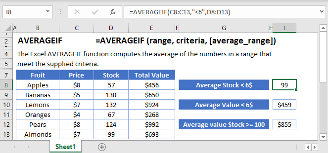
Returns the average (arithmetic mean) of all the cells in a range that meet a given criteria.

Syntax

AVERAGEIF(range, criteria, [average_range])

The AVERAGEIF function syntax has the following arguments:

• Range    Required. One or more cells to average, including numbers or names, arrays, or references that contain numbers.

• Criteria    Required. The criteria in the form of a number, expression, cell reference, or text that defines which cells are averaged. For example, criteria can be expressed as 32, «32», «>32», «apples», or B4.

• Average_range    Optional. The actual set of cells to average. If omitted, range is used.

Remarks

• Cells in range that contain TRUE or FALSE are ignored.

• If a cell in average_range is an empty cell, AVERAGEIF ignores it.

• If range is a blank or text value, AVERAGEIF returns the #DIV0! error value.

• If a cell in criteria is empty, AVERAGEIF treats it as a 0 value.

• If no cells in the range meet the criteria, AVERAGEIF returns the #DIV/0! error value.

• You can use the wildcard characters, question mark (?) and asterisk (*), in criteria. A question mark matches any single character; an asterisk matches any sequence of characters. If you want to find an actual question mark or asterisk, type a tilde (~) before the character.

• Average_range does not have to be the same size and shape as range. The actual cells that are averaged are determined by using the top, left cell in average_range as the beginning cell, and then including cells that correspond in size and shape to range. For example:

If range is	And average_range is	Then the actual cells evaluated are
A1:A5	B1:B5	B1:B5
A1:A5	B1:B3	B1:B5
A1:B4	C1:D4	C1:D4
A1:B4	C1:C2	C1:D4

Note: The AVERAGEIF function measures central tendency, which is the location of the center of a group of numbers in a statistical distribution. The three most common measures of central tendency are:

• Average     which is the arithmetic mean, and is calculated by adding a group of numbers and then dividing by the count of those numbers. For example, the average of 2, 3, 3, 5, 7, and 10 is 30 divided by 6, which is 5.

• Median     which is the middle number of a group of numbers; that is, half the numbers have values that are greater than the median, and half the numbers have values that are less than the median. For example, the median of 2, 3, 3, 5, 7, and 10 is 4.

• Mode     which is the most frequently occurring number in a group of numbers. For example, the mode of 2, 3, 3, 5, 7, and 10 is 3.

For a symmetrical distribution of a group of numbers, these three measures of central tendency are all the same. For a skewed distribution of a group of numbers, they can be different.

Examples

Copy the example data in the following table, and paste it in cell A1 of a new Excel worksheet. For formulas to show results, select them, press F2, and then press Enter. If you need to, you can adjust the column widths to see all the data.

Property Value	Commission
100000	7000
200000	14000
300000	21000
400000	28000
Formula	Description	Result
=AVERAGEIF(B2:B5,»<23000″)	Average of all commissions less than 23000. Three of the four commissions meet this condition, and their total is 42000.	14000
=AVERAGEIF(A2:A5,»<250000″)	Average of all property values less than 250000. Two of the four property values meet this condition, and their total is 300000.	150000
=AVERAGEIF(A2:A5,»<95000″)	Average of all property values less than 95000. Because there are 0 property values that meet this condition, the AVERAGEIF function returns the #DIV/0! error because it tries to divide by 0.	#DIV/0!
=AVERAGEIF(A2:A5,»>250000″,B2:B5)	Average of all commissions with a property value greater than 250000. Two commissions meet this condition, and their total is 49000.	24500

Example 2

Region	Profits (Thousands)
East	45678
West	23789
North	-4789
South (New Office)	0
MidWest	9678
Formula	Description	Result
=AVERAGEIF(A2:A6,»=*West»,B2:B6)	Average of all profits for the West and MidWest regions.	16733.5
=AVERAGEIF(A2:A6,»<>*(New Office)»,B2:B6)	Average of all profits for all regions excluding new offices.	18589

This Tutorial demonstrates how to use the Excel AVERAGEIF and AVERAGEIFS Functions in Excel and Google Sheets to average data that meet certain criteria.

AVERAGEIF Function Overview

You can use the AVERAGEIF function in Excel to count cells that contain a specific value, count cells that are greater than or equal to a value, etc.

To use the AVERAGEIF Excel Worksheet Function, select a cell and type:

(Notice how the formula inputs appear)

AVERAGEIF Function Syntax and Arguments:

=AVERAGEIF(range, criteria, [average_range])

range – The range of cells to count.

criteria – The criteria that controls which cells should be counted.

average_range – [optional] The cells to average. When omitted, range is used.

What is the AVERAGEIF function?

The AVERAGEIF function is one of the older functions used in spreadsheets. It is used to scan through a range of cells checking for a specific criterion, and then giving the average (aka the mathematical mean) if the values in a range that correspond to those values. The original AVERAGEIF function was limited to just one criterion. After 2007, the AVERAGEIFS function was created which allows a multitude of criteria. Most of the general use remains the same between the two, but there are some critical differences in the syntax that we’ll discuss throughout this article.

If you haven’t already, you can review much of the similar structure and examples in the COUNTIFS article <insert link>.

Basic example

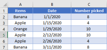
Let’s consider this list of recorded sales, and we want to know the average income.

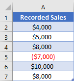
Because we had an expense, the negative value, we can’t just do a basic average. Instead, we want to average only the values that are greater than 0. The “greater than 0” is what will be our criteria in an AVERAGEIF function. Our formula to state this is

=AVERAGEIF(A2:A7, ">0")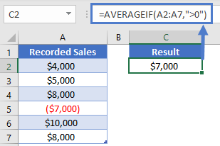

Two-column example

While the original AVERAGEIF function was designed to let you apply a criterion to the range of numbers you want to sum, much of the time you’ll need to apply one or more criteria to other columns. Let’s consider this table:

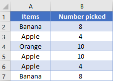
Now, if we use the original AVERAGEIF function to find out how many Bananas we have on average. We’ll put our criteria in cell D1, and we’ll need to give the range we want to average as the last argument, and so our formula would be

=AVERAGEIF(A2:A7, D1, B2:B7)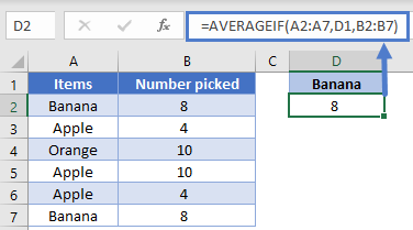

However, when programmers eventually realized that users wanted to give more than one criterion, the AVERAGEIFS function was created. In order to create one structure that would work for any number of criteria, the AVERAGEIFS requires that the sum range is listed first. In our example, this means that the formula needs to be

=AVERAGEIFS(B2:B7, A2:A7, D1)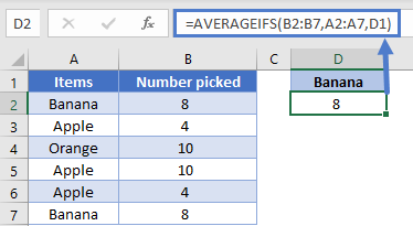

NOTE: These two formulas get the same result and can look similar, so pay close attention to which function is being used to make sure you list out all the arguments in the correct order.

Working with Dates, Multiple criteria

When working with dates in a spreadsheet, while it is possible to input the date directly into the formula, it’s best practice to have the date in a cell so that you can just reference the cell in a formula. For example, this helps the computer know that you’re wanting to use the date 5/27/2020, and not the number 5 divided by 27 divided by 2020.

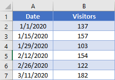
Let’s look at our next table recording the number of visitors to a site every two weeks.

We can specify the start and end points of the range we want to look at in D2 and E2. Our formula then to find the average the number of visitors in this range could be:

=AVERAGEIFS(B2:B7, A2:A7, ">="&D2, A2:A7, "<="&E2)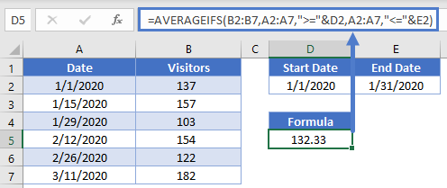

Note how we were able to concatenate the comparisons of “<=” and “>=” to the cell references to create the criteria. Also, even though both criteria were being applied to the same range of cells (A2:A7), you need to write out the range twice, once per each criterion.

Multiple columns

When using multiple criteria, you can apply them to the same range as we did with previous example, or you can apply them to different ranges. Let’s combine our sample data into this table:

We’ve setup some cells for the user to enter what they want to search for in cells E2 through G2. We thus need a formula that will add up the total number of apples picked in February. Our formula looks like this:

=AVERAGEIFS(C2:C7, B2:B7, ">="&F2, B2:B7, "<="&G2, A2:A7, E2)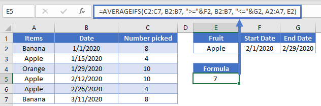

AVERAGEIFS with OR type logic

Up to this point, the examples we’ve used have all been AND based comparison, where we are looking for rows that meet all our criteria. Now, we’ll consider the case when you want to search for the possibility of a row meeting one or another criterion.

Let’s look at this list of sales:

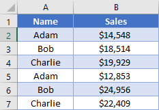
We’d like to add up the average sales for both Adam and Bob. First, a quick discussion about taking averages. If you have an uneven number of things such has 3 entries for Adam and 2 for Bob, you can’t simply take the average of each person’s sales. This is known as taking the average of averages, and you end up giving an unfair weighting to the item that has few entries. If this is the case with your data, you’d need to calculate an average the “manual” way: take the sum of all your items divided by the count of your items. To review how to do this, you can check out the articles here: <link to SUMIFS and COUNTIFS>

Now, if the number of entries is the same, such as in our table, then you have a couple options you can do. The simplest is to add two AVERAGEIFS together, like so, and then divide by 2 (the number of items in our list)

=(AVERAGEIFS(B2:B7, A2:A7, "Adam")+AVERAGEIFS(B2:B7, A2:A7, "Bob"))/2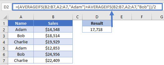

Here, we’ve had the computer calculate our individual scores, and then we add them together.

Our next option is good for when you have more criteria ranges, such that you don’t want to have to rewrite the whole formula repeatedly. In the previous formula, we manually told the computer to add two different AVERAGEIFS together. However, you can also do this by writing your criteria inside an array, like this:

=AVERAGE(AVERAGEIFS(B2:B7, A2:A7, {"Adam", "Bob"}))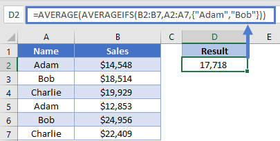

Look at how the array is constructed inside the curly brackets. When the computer evaluates this formula, it will know that we want to calculate an AVERAGEIFS function for each item in our array, thus creating an array of numbers. The outer AVERAGE function will then take that array of numbers and turn it into a single number. Stepping through the formula evaluation, it would look like this:

=AVERAGE(AVERAGEIFS(B2:B7, A2:A7, {"Adam", "Bob"}))
=AVERAGE(13701, 21735)
=17718

We get the same result, but we were able to write out the formula a bit more succinctly.

Dealing with blanks

Sometimes your data set will have blank cells that you need to either find or avoid. Setting up the criteria for these can be a little tricky, so let’s look at another example.

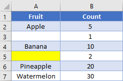
Note that cell A3 is truly blank, while cell A5 has a formula returning a zero-length string of “”. If we want to find the total average of truly blank cells, we’d use a criterion of “=”, and our formula would look like this:

=AVERAGEIFS(B2:B7,A2:A7,"=")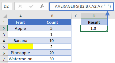

On the other hand, if we want to get the average for all cells that visually looks blank, we’ll change the criteria to be “”, and the formula looks like

=AVERAGEIFS(B2:B7,A2:A7,"")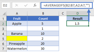

Let’s flip it around: what if you want to find the average of non-blank cells? Unfortunately, the current design won’t let you avoid the zero-length string. You can use a criterion of “<>”, but as you can see in the example, it still includes the value from row 5.

=AVERAGEIFS(B2:B7,A2:A7,"<>")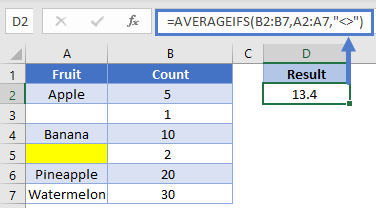

If you need to not count cells containing zero length strings, you’ll want to consider using the LEN function inside a SUMPRODUCT <link to SUMPRODUCT article).

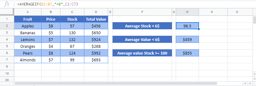
AVERAGEIF in Google Sheets

The AVERAGEIF Function works exactly the same in Google Sheets as in Excel:

AVERAGEIF and AVERAGEIFS are both Statistical functions n Microsoft Excel. In this post, we will take a look at their syntax and how to use them.

The AVERAGEIF function evaluates the average of all numbers in a range that meet a given criterion. The formula for the AVERAGEIF is:

 Averageif (Range, criteria, [average_range])

The AVERAGEIFS function returns the average of all numbers in a range that meets multiple criteria. The formula for AVERAGEIFS is:

 Averageifs (average_range, criteria_range1, criteria1[criteria_ range2, criteria2] …)

Syntax of AVERAGEIF and AVERAGEIFS

AVERAGEIF

• Range: is the group of cells you want to average. The Range is required.
• Criteria: The Criteria is used to verify which cells to average. Criteria are required.
• Average_range: The Range of cells to average. When absent, the range parameter will be average instead. Average_range is optional.

AVERAGEIFS

• Average_range: The Average_ Range is one or more cells to average. Average_range is required.
• Range: the group of cells you want to average. The Range is required.
• Criteria_range1: The first Range to evaluate the related criteria. The first Criteria_range1 is required, but the second criteria_ range is optional.
• Criteria 1: The Criteria verify which cells to average. The first criteria are required. The second criteria or any criteria after is optional.

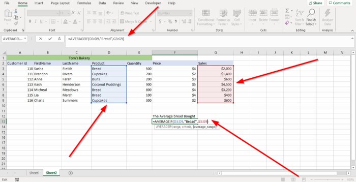
First, we are going to click the cell where we want the Average. Then type =Averageif bracket.

Inside the bracket, we will type the Range because the Range of cells contains the data we want to average.

In this tutorial, we will type the cell (D3:D9), or we can click on the cell in the column that we want to average and drag it to the end; this will automatically place the range of cells in the formula.

Now, we are going to enter the Criteria; the criteria validate which cells to average. We are going to use Bread in this tutorial because it is what we are looking for.

We are going to enter the Average_ range. We will type G3:G9 because these cells contain the sales we want to average; then close the bracket.

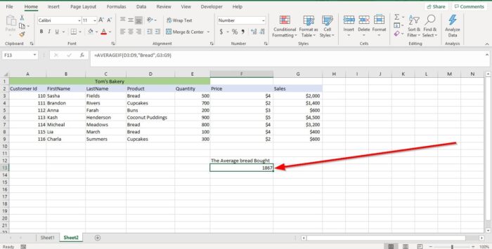
Press Enter, you will see the result.

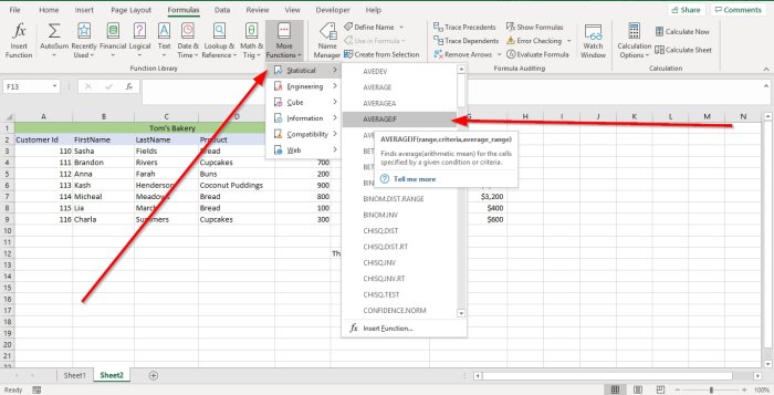
The other option is to go to Formulas. In the Function Library group, select More Functions. In the drop-down menu list, select Statistical in its menu choose AVERAGEIF. A Function Argument dialog box will appear.

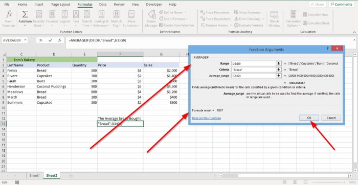
In the Function Arguments dialog box, where you see Range, type D3:D9 into its entry box.

In the Function Arguments dialog box, where you see Criteria, type “Bread” into the criteria entry box.

In the Function Arguments dialog box, where you see Average_range, type G3:G9 into its entry box.

Click OK and you will see your result.

Read: How to use SUMIF and SUMIFS Functions in Excel

How to use AVERAGEIFS in Excel

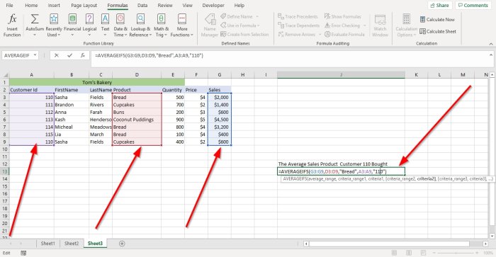
In this tutorial, we are going to look up the average sale of products bought by customer 110.

Click the cell where you want the result in, then type =Averageif, bracket.

In the bracket type G3:G9, this is the Average_range.

Now we are going to type the Criteria_range1. Type D3:D9, this range of cells contain the data we are looking for.

We will type the Criteria1, which is” Bread” because it is the product we are looking for.

We are going to fine Criteria_range2, which is A3:A9 because we want to identify the customer.

We will enter Criteria2, which is“110,” because this is the ID number of the customer we are looking for.

Press Enter and you will see your result.

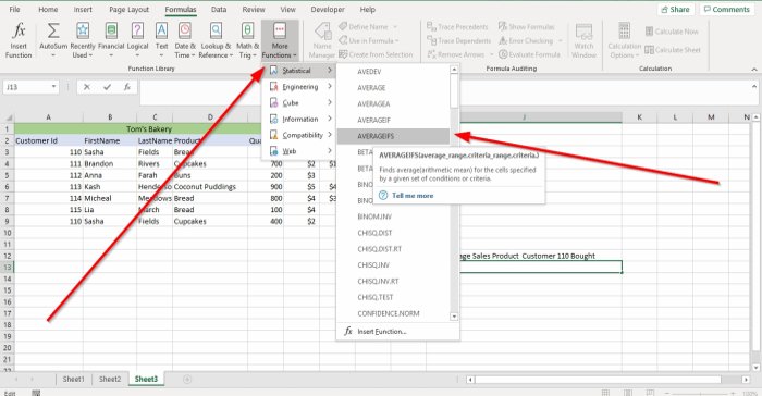
The other option is to go to Formulas. In the Function Library group, select More Functions. In the drop-down menu list, select Statistical in its menu select AVERAGEIFS; and a Function Argument dialog box will appear.

In the Function Arguments dialog box, where you see Average_range. Type G3:G9 in its entry box.

In the Function Arguments dialog box, where you see Criteria_range1. Type D3:D9 in its entry box.

In the Criteria1 entry box, type Bread.

In the Criteria_range2 entry box, type A3:A9.

In the Criteria2 entry box, type “110” because we are looking for the customer id 110.

Click OK. You will see the result.

Read next: How to use the IF Function in Excel.

Let’s say that a baby learning to crawl is an analogy for learning the AVERAGE function in Excel.

Then learning the AVERAGEIF function is like learning to walk, and learning the AVERAGEIFS function is like learning to run.

So, lace up your shoes and get ready to run 🙂

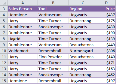
We’ll be using the table below in this tutorial. Inspired by my 5 year olds current obsession with the first Harry Potter movie.

Baby steps first:

Excel AVERAGE Function

=AVERAGE(your_data_range)

=AVERAGE(D4:D15)

=$271.58

As you can see, the Average function is fairly straight forward in that it simply averages a range of cells.

But there are some things you should know about how it works:

If one of the cells is blank it doesn’t include it in the number to average.

For example, there are 12 cells in our range D4:D15. So the AVERAGE function is actually summing the range of cells ($3,259), and then dividing them by 12 to get an average of $271.58.

But if cell D5 was blank it would sum the range of cells (and get $3,084) and divide them by 11 to get $280.36.

On the other hand, if cell D5 contained a zero it would still divide the sum by 12.

Excel AVERAGEIF Function

What if we wanted to get the average sales if the salesperson was Hermione?

That’s where the AVERAGEIF function comes into play. It allows you to average data in one range of cells where the data in another range matches a certain criteria.

The AVERAGEIF syntax is a bit different:

=AVERAGEIF(range, criteria, [average_range])

Where ‘range’ is the range containing your criteria, and [average_range] is the range of cells containing the values you want to average.

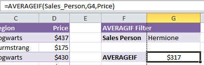
Let’s use the data below to find the average sales for Hermione.

Our formula would be:

=AVERAGEIF(A4:A15,”Hermione”,D4:D15)

=$317

In English;

=AVERAGE(referring to the range A4:A15, find Hermione, and average the values in the range D4:D15)

Note: the ranges of data must be the same size. In this example both refer to rows 4 to 15.

However, it wouldn’t work if one referred to rows 4 to 10 and the other referred to rows 4 to 15.

The limitation of the AVERAGEIF function is that you can only use one criterion.

AVERAGEIFS Function Syntax

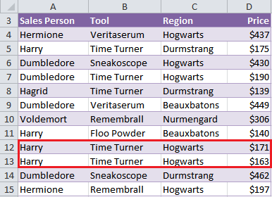
Whereas if you wanted to find the AVERAGE sales by ‘Harry’ of the product ‘Time Turner’ in the ‘Hogwarts’ region you’d need to use the AVERAGEIFS function.

=AVERAGEIFS(average_range, criteria_range1, criteria1, criteria_range2, criteria2,…)

Using our example data again our AVERAGEIFS function would be:

=AVERAGEIFS(D4:D15,A4:A15,"Harry",B4:B15, "Time Turner",C4:C15,"Hogwarts")

=$167

Two rows match our criteria:

Download the Workbook

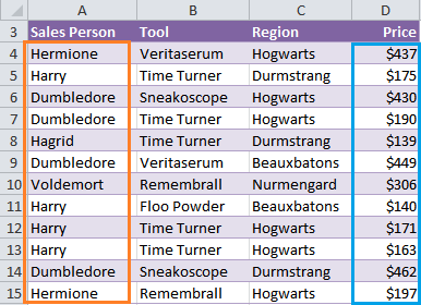
Enhancement 1: Named Ranges

Notice in the formula bar how the first and last arguments of the syntax is ‘Sales_Person’ and ‘Price’ rather than a the cell ranges A4:A15 for Sales_Person and D4:D15 for Price?

This is called a named range and they make building your formulas quick and also easy to interpret later on.

Enhancement 2: Data Validation

In the AVERAGEIFS function I’ve also used named ranges. Plus I’ve used a data validation list or drop down list as they’re sometimes known as seen in action in the animation above.

The formula in cell G16 is:

=AVERAGEIFS(Price,Sales_Person,G11,Tool,G12,Region,G13)

This allows me to choose the criteria from the data validation lists in cells G11, G12 and G13 and the AVERAGEIFS formula will dynamically update to show the results for the new criteria.

Want to learn more tricks like this?

It’s techniques like this that I teach in my dashboard course to create reports that are interactive for the report recipient.

These features make your colleagues love you, because when you give them reports like this they are in control of getting the information they need quickly and easily.

And they save you time because you don’t have to create myriad of reports to cover every scenario.

It’s a win, win.

Click here to learn more about Excel Dashboard reports and how you can build interactive features into them.

Microsoft Excel – AVERAGEIFS, AVERAGEIF, and AVERAGE functions are useful to calculate the Average value.

Microsoft Excel provides a good number of Functions to enable us to deal with Spreadsheet data. In this article, I am going to explain, AVERAGE, AVERAGEIF, and AVERAGEIFS functions. Before we start looking into these functions; lets’ understand, why an Average is required.

Why Average is required?

An average is required, to calculate the Central Value of the Data Set. For example, when you report your Company’s financials; you report Average data; instead of each and every detail. By seeing the Average results, people can understand; how the company is performing. Based on that the investors will start investing in the Company for growth. That means Average results are really helpful when showing financial results.

Another simple example is, we have 100 people, and everyone has different quantities of Apples. If someone asks, how many Apples the people have. Do you report the Average count? Or the Apple count each person has? We usually report the Average count. We calculate the Average, by summing all the Apples, divided by, the count of people (here it is 100). Now we know, on Average; each person has the count of Apples. This is easy to report; instead of reporting an individual’s Apple count.

Lets’ discuss, how we use them in Microsoft Excel.

AVERAGE function

Microsoft Excel provides the AVERAGE function; which gives the mean of the selected data.

Syntax: AVERAGE (number1, [number2], ...) OR
Syntax: AVERAGE (range)

For example, the average of 1, 2, 3, 4 is (1+2+3+4)/4 = 2.5. That means AVERAGE is the DIVISION of the SUM of the whole data set and COUNT of the whole data set. It considers, all the data set values to calculate the Average.

The AVERAGE function, allows multiple values separated by a comma (“,”) or range of values; to calculate the Average.

Lets’ take sample data; showing, which Positions the Sample Web Site pages are displaying in Search Results. We will calculate, Average Position, by using the AVERAGE function. These results are helpful to SEOs to optimize the Web Site for better positioning in Search Engine results.

Positions	Formula	Average Position
22.3	=AVERAGE(A2:A8)	12.46
10.9
10.8
14.4
7.9
9.4
11.5

Note that, I have colored the entries which are included in the formula, to calculate the Average.

I don’t want to do the Average, on the larger Positions; how do we do this.? The AVERAGE function doesn’t allow conditions. Another function, Excel provides, is AVERAGEIF; which allows applying conditions to select the data to find the Average.

AVERAGEIF function

Microsoft Excel provides another variation of the AVERAGE function; which is the AVERAGEIF function, used to exclude some data in the data set depending on some criteria.

Syntax: AVERGAEIF (range, criteria) OR
Syntax: AVERAGEIF (criteria_range, criteria, [average_range])

For example, the average of 0, 1, 2, 3, 4 is (0+1+2+3+4)/5 = 2. If we exclude 0, the Average would be 2.5.

By using the AVERAGE function, we can not omit the values. To exclude some values (for example, 0 here) from the data set, the AVERAGEIF function will be useful.

Lets’ take the above sample data; adding “Clicks” sample data to it. Clicks data represents, that the User clicks on the Web Site links; displayed in the Search Result. If your Web Site is appearing on the first page, of Search Results; you will have more Visitors (more Clicks) to your site.

I want to omit the Positions which are > 20 and want to find the Average Position in Search Results. We need to use the AVERAGEIF function, and the criteria should be, to consider the Position values which are below 20 (which means, omitting the positions which are >=20).

Positions	Clicks	Formula	Average Position
22.3	0	=AVERAGE(A2:A8)	12.46
10.9	3
10.8	8	=AVERAGEIF(A2:A8, “<20”)	10.82
14.4	5
7.9	5
9.4	7
11.5	5

Observe that, from the above data; position 22.3 was omitted and only the rest of the positions were considered for the Average position. Because those values are “< 20”; satisfied the given condition.

Does it possible to get the Average Position, based on the Clicks data, instead of the Positions data.? Yes. The second Syntax, mentioned above, is useful for this. So far, we have applied the condition to the same data; from which we want to get the Average. But AVERAGEIF allows us to apply the condition on the different data ranges; to get the Average. Again, I am mentioning the second Syntax here:

Syntax: AVERAGEIF (criteria_range, criteria, [average_range])

where:

The “criteria_range” is the condition range on which you want to apply the condition;

The “criteria” is the condition to apply on the data range mentioned in “criteria_range“;

“average_range” is the range from which you want to find the Average.

Lets’ find the Average Position if the Website has any Visitors. Here the “criteria_range” is Clicks, and the condition is “>0”; that means, Website has any Visitors (or Clicks). We need to get the Average Position; so, the “average_range” is Positions. The formula & the result looks like below:

Positions	Clicks	Formula	Average Position
22.3	0	=AVERAGE(A2:A8)	12.46
10.9	3
10.8	8	=AVERAGEIF(A2:A8, “<20”)	10.82
14.4	5	=AVERAGEIF(B2:B8, “>0”, A2:A8)	10.82
7.9	5
9.4	7
11.5	5

You must notice, how the data was filtered (from the above condition); based on the data in Clicks; to find the Average Position from the Positions data.

I hope the AVERAGEIF function is clear to you. It considers only one criterion or condition; to calculate the Average value. How about, if we have multiple conditions to calculate the Average.? Hence we have the AVERAGEIFS function.

I recommend you understand completely, the AVERAGE & AVERAGEIF functions, before moving to AVERAGEIFS.

AVERAGEIFS function

Microsoft Excel provides another interesting variation of the AVERAGE  function is the AVERAGEIFS function. This function allows multiple criteria or conditions to calculate the Average value. Each condition should be applied in a specified range.

Syntax: AVERAGEIFS (average_range, criteria_range1, condition1, [criteria_range2, condition2], ...)

Lets’ take the above sample data, and add the “Impressions” sample data to it. The sample data looks like below. Impressions represent how many times the Web Site appears in the Search Result; Clicks data represents the number of visitors to the Web Site.

Based on the Position in the Search Results, the Web Site Impressions, and the site Visitors may increase.

Lets’ calculate the Average Position value; based on the conditions: Should have visitors to the Web Site & at least 50 Impressions of the site. The formula looks like below:

Positions	Clicks	Impressions	Formula	Average Position
22.3	0	20	=AVERAGE(A2:A8)	12.46
10.9	3	40
10.8	8	48	=AVERAGEIF(A2:A8, “<20”)	10.82
14.4	5	89
7.9	5	58
9.4	7	70
11.5	5	72	=AVERAGEIFS(A2:A8, B2:B8,”>0″, C2:C8, “>50”)	10.8

Have you noticed the above data.? Only a few entries from Positions were satisfied with the above conditions; and I have colored them, those Positions. 

Happy reading!

I may explain more Excel functions in upcoming Articles.

I hope you liked this Article. Please give your feedback through the below Comments.

🙂 Sahida