Auto numbering in excel

Automatically number rows

Unlike other Microsoft 365 programs, Excel does not provide a button to number data automatically. But, you can easily add sequential numbers to rows of data by dragging the fill handle to fill a column with a series of numbers or by using the ROW function.

Tip: If you are looking for a more advanced auto-numbering system for your data, and Access is installed on your computer, you can import the Excel data to an Access database. In an Access database, you can create a field that automatically generates a unique number when you enter a new record in a table.

What do you want to do?

Fill a column with a series of numbers
Use the ROW function to number rows
Display or hide the fill handle

Fill a column with a series of numbers

Select the first cell in the range that you want to fill.
Type the starting value for the series.
Type a value in the next cell to establish a pattern.

Tip: For example, if you want the series 1, 2, 3, 4, 5…, type 1 and 2 in the first two cells. If you want the series 2, 4, 6, 8…, type 2 and 4.
Select the cells that contain the starting values.

Note: In Excel 2013 and later, the Quick Analysis button is displayed by default when you select more than one cell containing data. You can ignore the button to complete this procedure.
Drag the fill handle across the range that you want to fill.

Note: As you drag the fill handle across each cell, Excel displays a preview of the value. If you want a different pattern, drag the fill handle by holding down the right-click button, and then choose a pattern.

To fill in increasing order, drag down or to the right. To fill in decreasing order, drag up or to the left.

Tip: If you do not see the fill handle, you may have to display it first. For more information, see Display or hide the fill handle.

Note: These numbers are not automatically updated when you add, move, or remove rows. You can manually update the sequential numbering by selecting two numbers that are in the right sequence, and then dragging the fill handle to the end of the numbered range.

Use the ROW function to number rows

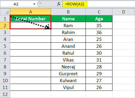
In the first cell of the range that you want to number, type =ROW(A1).

The ROW function returns the number of the row that you reference. For example, =ROW(A1) returns the number 1.
Drag the fill handle across the range that you want to fill.

Tip: If you do not see the fill handle, you may have to display it first. For more information, see Display or hide the fill handle.

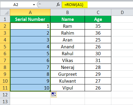
These numbers are updated when you sort them with your data. The sequence may be interrupted if you add, move, or delete rows. You can manually update the numbering by selecting two numbers that are in the right sequence, and then dragging the fill handle to the end of the numbered range.
If you are using the ROW function, and you want the numbers to be inserted automatically as you add new rows of data, turn that range of data into an Excel table. All rows that are added at the end of the table are numbered in sequence. For more information, see Create or delete an Excel table in a worksheet.

To enter specific sequential number codes, such as purchase order numbers, you can use the ROW function together with the TEXT function. For example, to start a numbered list by using 000-001, you enter the formula =TEXT(ROW(A1),»000-000″) in the first cell of the range that you want to number, and then drag the fill handle to the end of the range.

Display or hide the fill handle

The fill handle displays by default, but you can turn it on or off.

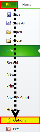
In Excel 2010 and later, click the File tab, and then click Options.

In Excel 2007, click the Microsoft Office Button , and then click Excel Options.
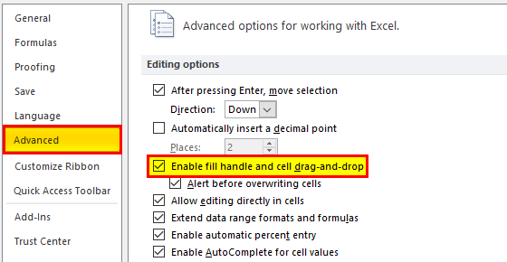
In the Advanced category, under Editing options, select or clear the Enable fill handle and cell drag-and-drop check box to display or hide the fill handle.

Note: To help prevent replacing existing data when you drag the fill handle, ensure the Alert before overwriting cells check box is selected. If you do not want Excel to display a message about overwriting cells, you can clear this check box.

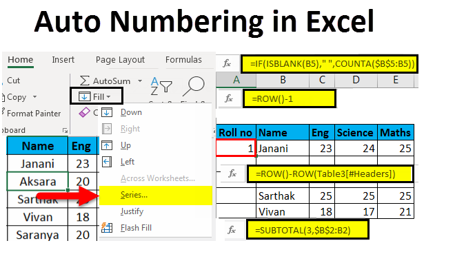
Automatic Numbering in Excel

Numbering means giving serial numbers or numbers to a list of data. In Excel, no special button is provided that offers numbering for our data. As we already know, Excel does not provide a method, tool, or button to provide the sequential number to a list of data, which means we need to do it manually.

Automatic Numbering in Excel
- How to Auto Number in Excel?
- Top 3 ways to get Auto Numbering in Excel
  - #1 – Filling the Column with a Series of Numbers
  - #2 – Use ROW() Function
  - #3 – Using Offset() Function
- Things to Remember about Auto Numbering in Excel
- Auto Numbering in Excel Video
- Recommended Articles

How to Auto Number in Excel?

We must remember that our AutoFill functionAutoFill in excel can fill a range in a specific direction by using the fill handle.read more is always turned on to create auto numbering in Excel. By default, it is turned on. But in any case, if it is not enabled or mistakenly disabled “AutoFill,” here is how we can re-enable it.

Now we have checked that the “Autofill” is enabled. There are three methods for Excel auto-numbering:

Fill a column with a series of numbers.
Using the Row() function.
Using the Offset() function.

The following are the steps for enabling fill handle and cell drag and drop: –

In the “File” tab, go to “Options.”
In the advanced section, check the “Enable fill handle and cell drag and drop” in Excel under the editing options.

Top 3 ways to get Auto Numbering in Excel

There are various ways to get automatic numbering in Excel.

You can download this Auto Numbering Excel Template here – Auto Numbering Excel Template

Fill a column with a series of numbers.
Use Row() function
Use Offset() Function

Let us discuss all the above methods by examples.

#1 – Filling the Column with a Series of Numbers

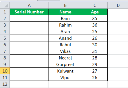
We have the following data:

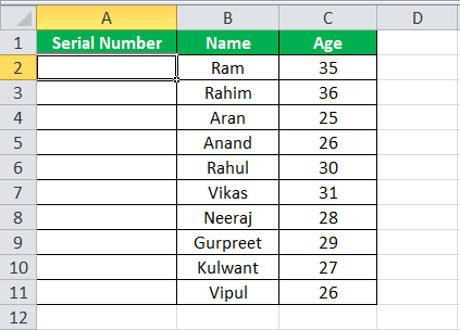
We will insert automatic numbers in Excel “column A” following the below steps:

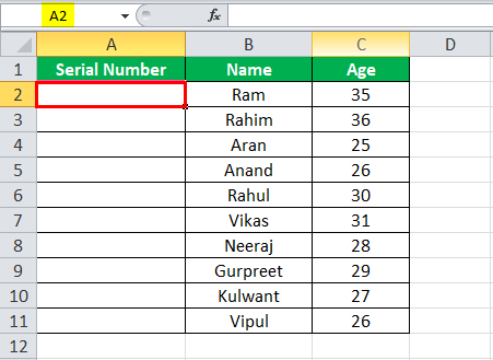
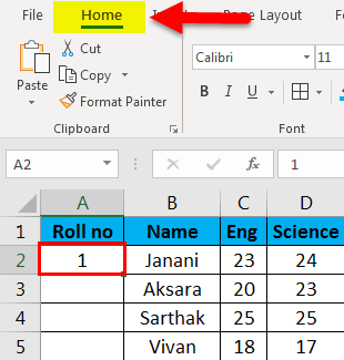
We can select the cell we want to fill. In this example, we will choose cell A2.
We will write the number we want to start with. Let it be 1, fill the next cell in the same column with another number, and let it be 2.

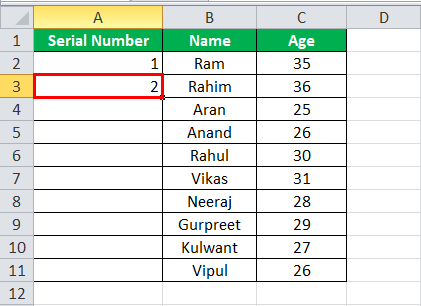
To start a pattern, we have made the numbering 1 in cell A2 and 2 in cell A3. Next, we will select the starting values, i.e., cells A2 and A3.

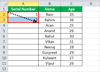
The arrow shows the pointer (dot) in the selected cell. Then, click on it and drag it to the desired range, cell A11.

Now, we have sequential numbering for our data.

#2 – Use ROW() Function

We will use the same data to demonstrate the sequential numbering by the Row() functionThe row function in Excel is a worksheet function that displays the current row index number of the selected or target cell. The syntax to use this function is as follows: =ROW( Value ).read more.

Below is our data:

We select the specific cell where we want to start our automatic numbering in Excel (cell A2 in this case).

We type ROW() in cell A2 and press “Enter.”

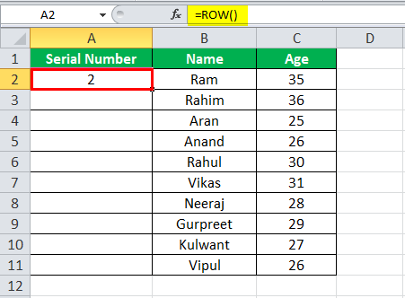
As a result, it gave us the numbering from number 2 since the Row function throws the number for the current row.

To avoid the above situation, we can give the reference row to the Row function.

Next, we click on the pointer or the dot in the selected cell and drag it to the desired range for the current scenario to cell A11.

We have automatic numbering in Excel for the data using the Row() function.

#3 – Using Offset() Function

We can also achieve auto numbering in Excel using the Offset() functionThe OFFSET function in excel returns the value of a cell or a range (of adjacent cells) which is a particular number of rows and columns from the reference point. read more also.

Let us use the same data to demonstrate the Offset function. Below is the data:

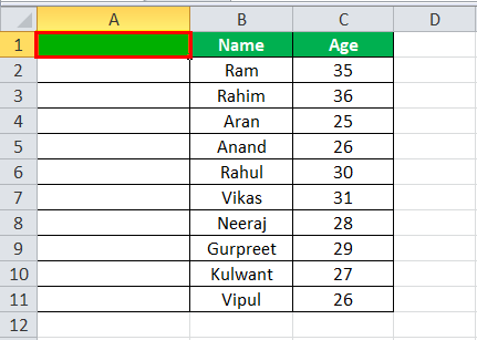
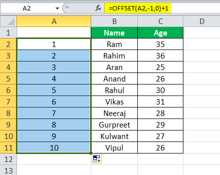
As we can see, we have removed the text written in cell A1 “Serial Number,” as the reference needs to be blank while using the Offset function.

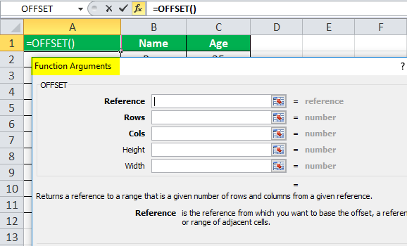
The above screenshot shows the function arguments used in the Offset function.

In cell A2, we type offset(A2,-1,0)+1 for the automatic numbering in Excel.

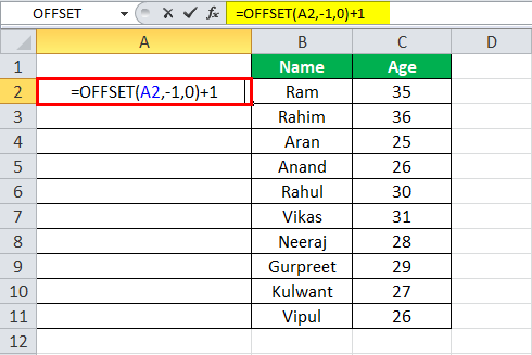
A2 is the current cell address, which is the reference.

Press the “Enter” key. It will insert the first number.

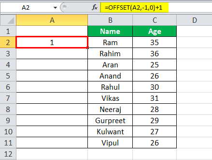
Now, we select cell A2 and drag it down to cell A11.

So, now we have sequential numbering using the Offset function.

Things to Remember about Auto Numbering in Excel

Excel does not auto-provide auto-numbering.
Do not forget to check for the enabled “AutoFill” option.
While filling a column with a series of numbers, we must make a pattern. We can use the starting values as 2 or 4 to create even sequential numbering.

Auto Numbering in Excel Video

Auto Numbering in Excel is used to generate the number automatically in a sequence or in some pattern. We can fill and drag the numbers down the limit we want. We can enable the option of Auto numbering available in the Excel Options’ Advanced tab. In another way, we can use the ROW function. This function starts counting the row by returning its number as per the number mentioned in Row numbers. We can also generate auto numbers by adding +1 to the number located above.

Methods to number rows in Excel

The auto-numbering of rows in excel would depend on the kind of data used in excel. For Example –

- A continuous dataset that starts from a different row.
- A dataset that has a few blank rows and only filled rows to be numbered.

You can download this Auto Numbering excel Excel Template here – Auto Numbering excel Excel Template

Methods are as follows:

- - By Using the Fill handle
  - By Using Fill series
  - By Using the CountA function
  - By Using Row Function
  - By Using Subtotal for filtered data
  - By Creating an Excel Table
  - By adding one to the previous row number

1. Fill handle Method

It helps in auto-populating a range of cells in a column in a sequential pattern, thus making the task easy.

Steps to be followed:

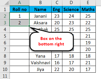
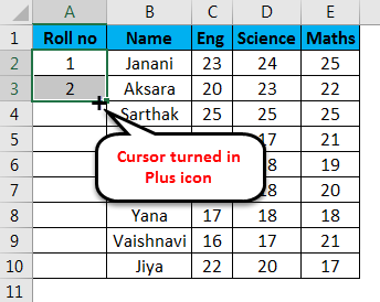
- - Enter 1 in the A2 cell and 2 in the A3 cell to make the pattern logical.

- - There is a small black box on the bottom right of the selected cell.
  - The moment the cursor is kept on the cell, it changes to a plus icon.

- - Drag the + symbol manually till the last cell of the range or double click on the plus icon, i.e. fill handle; a number will appear automatically in serial order.

Note:

- - The row number will get updated in case of addition/deletion of row(s)
  - It identifies the pattern of the series from the two filled cells and fills the rest of the cells.
  - This method does not work on an empty row.
  - Numbers are listed serially; however, the roman number format and alphabet listing are not considered.
  - The serial number inserted is a static value.

2. Fill Series Method

This method is more controlled and systematic in numbering the rows.

Steps to be followed:

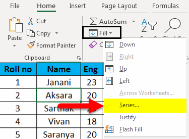
- - Enter 1 in the A2 cell -> go to ‘Home tab of the ribbon.

- - Select “Fill”drop-down -> Series

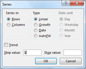
- - Series dialog box will appear.

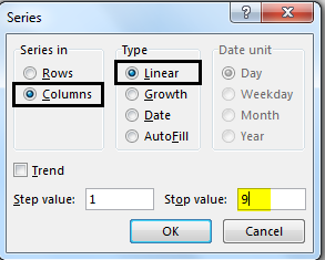
- - Click the Columns button under Series and insert number 9 in the Stop value: input box. Press OK. The number series will appear.

Fill the first cell and apply the below steps.

- - This method works on an empty row also.
  - Numbers are listed serially, but the roman number and alphabets listing are not considered.
  - The serial number inserted is a static value. A serial number does not change automatically.

3. COUNTA function Method

The COUNTA function is used in numbering only those rows that are not empty within a range.

Steps to be followed:

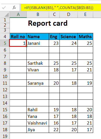
Select the cell A5, corresponding to the first non-empty row in the range and paste the following formula –

=IF(ISBLANK(B5),” “,COUNTA($B$5:B5))

Then, the cell gets populated with the number 1. Then drag the fill handle (+) to the last cell within the column range.

- - The number in a cell is dynamic in nature. When a row is deleted, existing serial numbers are automatically updated, serially.
  - Blank rows are not considered.

4. Row function method

The Row function can be used to get the row numbering.

Follow the below process.

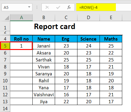
Enter the ROW() function and subtract 1 from it to assign the correct row number. ROW() calculates to 2; however, we want to set the cell value to 1, being the first row of the range; hence 1 is subtracted. Hence formula will be,

=ROW()-1

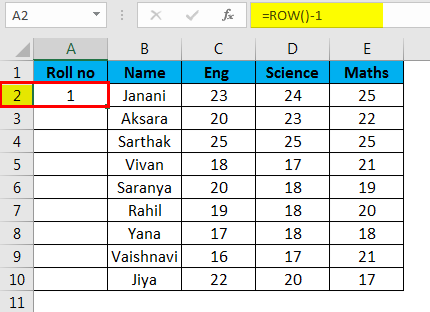
If the row starts from 5^th, the formula will change accordingly, i.e. =ROW() – 4

- - The row number will get updated in case of the addition/deletion of row(s).
  - It is not referencing any cell in the formula and will automatically adjust the row number.
  - It will display the row number even if the row is blank.

5. SUBTOTAL For Filtered Data

The SUBTOTAL function in Excel helps in the serial numbering of a filtered dataset copied into another datasheet.

Steps to be followed:

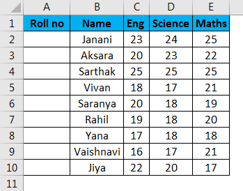
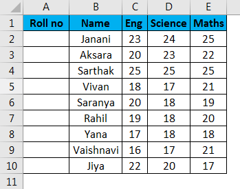
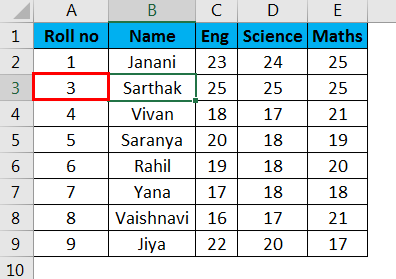
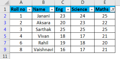
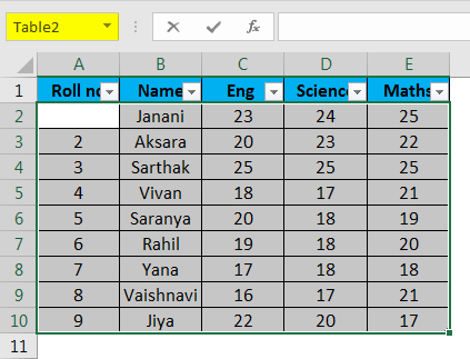
Here is a dataset which we intend to filter for marks in Maths greater than or equal to 20.

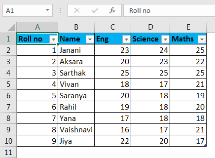
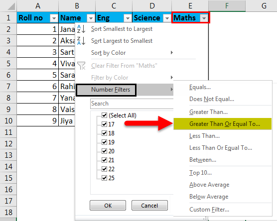
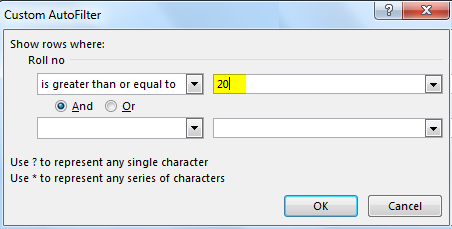
Now we will copy this filtered data into another sheet and delete the “Roll no” serial values.

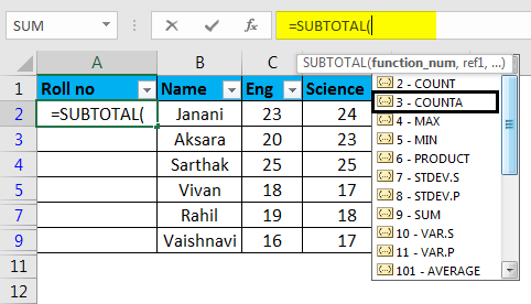
Then, select the first cell of the column range and use the ‘SUBTOTAL’ function wherein the first argument is 3, denoting ‘COUNT A’.

=SUBTOTAL(3,$B$2:B2)

This will populate the cell with a value of 1.

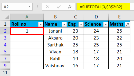
Now, with the selected cell, drag the fill handle (+) downwards along the column. This will populate the rest of the cells serially.

- - The SUBTOTAL function is useful in rearranging the row count, serially, of a copied filtered dataset in another sheet.
  - The serial numbers are automatically adjusted on the addition/deletion of rows.

6. By creating an Excel Table

Here, tabular data is converted into the Excel table.

Steps to be followed:

Firstly, select the whole dataset ->go to Insert Tab->Click on Table icon(CTRL+T) under Table group

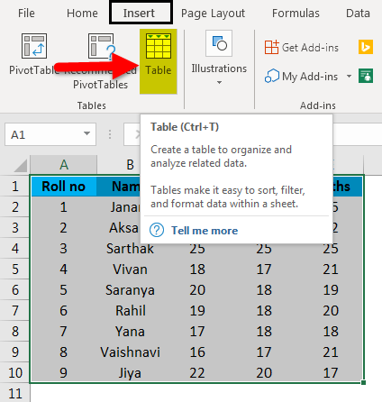
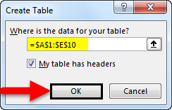
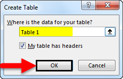
Create Table dialog box will appear. Specify range or table name

Click OK.

Tabular data is converted into Excel Table (named as Table 3).

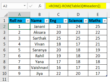
In the A2 cell, enter the formula.

Formula:

=Row()-Row(Table[#Header])

This will automatically fill the formula in all the cells.

- - Row numbering will automatically adjust and update on the addition/deletion of rows.

7. By adding one to the previous row number

Subsequent rows get incremented by 1.

Steps to be followed:

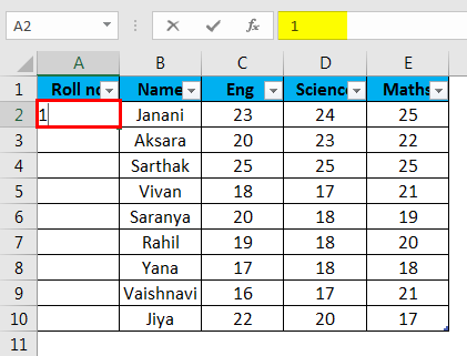
As seen in the attached screenshot, enter 1 in cell A2 of the first row.

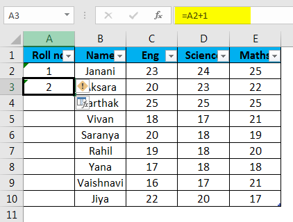
- - Enter =A2+1 in cell A3

- - Select A3 and drag the fill handle (+) to the last cell within the range. This will auto-populate the remaining cells.

- - The cell value is relative to the previous cell value.
  - Does not update serial number automatically on addition/deletion of rows.

Things to Remember about Auto Numbering in Excel

- - The best way for auto numbering in excel depends on the type of data set you to have to enable.
  - Auto Numbering in Excel is not an inbuilt function.
  - Ensure to check if the Fill option is enabled for Auto Numbering in Excel.

Conclusion

There are different ways for Auto Numbering in Excel and number rows in serial order in excel. Some of the methods will do static numbering, whereas others would do dynamic updates on the addition/deletion of rows.

You can download this Auto Numbering Excel Excel Template here – Auto Numbering Excel Template.

How to Auto-Number Cells with a Regular Pattern

For this method, you set your starting number in one cell and the next number in the series in the next cell.

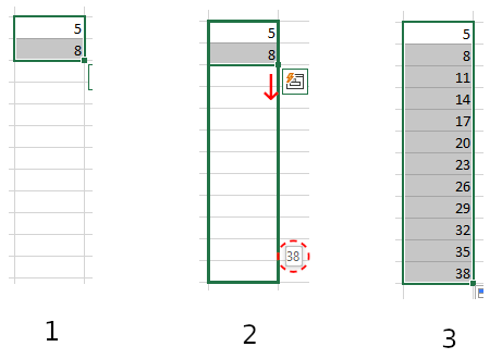
Once you have two adjacent cells filled with your two starting numbers, you can select those two cells, click on the handle in the bottom right corner of the green outline, and drag to select all the cells that you want to follow your pattern.

A useful tooltip appears near the bottom right corner of the green outline to show what the last number in the series would be if you released at that point.

So, if you want to start with the number 5 and increment by 3 until 38, you would write 5 in your first cell, and 8 in the next cell. You would then select the cells containing the 5 and the 8, click on the handle, and drag to select the other cells until you see 38 appear in the tooltip. Then you can release, and the numbers will be filled in automatically.

1) Select the cells. 2) Drag the handle on the outline (you can also see the tooltip with the last number in the series) 3) Release

The numbers can also be formatted in descending order: if you start with 7 and then enter 5, the pattern will continue with 3, 1, -1, and so on.

You can also do the same with rows instead of columns. Fill in two consecutive cells in a row with the start of your pattern, then select them and drag the outline horizontally across those cells that you want to continue that pattern. It’ll automatically fill in those numbers.

You can also do the same going upward – fill two cells, select them, click the handle and drag upward to fill the cells above your two starting cells.

Note: this will always add numbers that are evenly spaced in the pattern you’ve started. It won’t work with other kinds of number progressions.

How to Auto-Number Cells Using the ROW() Function

If you have data that can be sorted in different ways (say, a list of names — alphabetically, etc), it’s annoying if the numbering of your lines gets scrambled when you’re sorting other data.

To avoid that, you can dynamically number your rows using the ROW() function.

In the cell where you want the numbering to start, write =ROW(A1). This will produce the number 1 in the cell.

Select the cell and drag the outline from the handle in the corner to populate the same formula in the rest of the cells (or, if you are adding the line numbers near a block of data already present, you can just double-click on the handle on the corner of the selection).

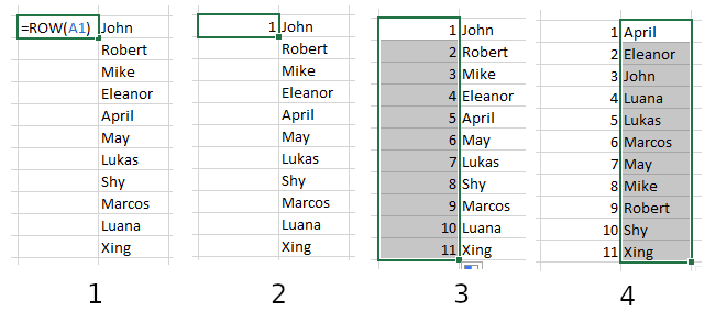
1) Write =ROW(A1) in your first cell, 2) It will appear as the number1, 3) Click and drag or double-click to fill all other cells. 4) Now if you sort the data, the line numbers will stay in order.

If you want to have a different regular pattern, you can use a bit of math: to have numbers spaced by 2, you can write =ROW(A1) * 2 in the first cell, and then proceed with the same steps as above. This will produce the numbers 2, 4, 6…and so on.

If you want to change the starting point of the pattern – to maybe have only odd numbers, for example – you can subtract one: =ROW(A1) * 2 - 1, this will produce the numbers 1, 3, 5, 7…

As a general formula, to get any pattern you can write =ROW(A1) * a + b. a is used to determine the step, and b (it can be either a positive or negative number) is used to change the starting point of the pattern.

If you want to number your columns, you can use the COLUMN() function in the same way as the ROW(). Just fill in your first cell with =COLUMN(A1) , select the cell, then expand the selection to the rest of the cells you want your numbers to be in.

Note: if you add or delete rows, you will need to set the auto-numbering again by selecting the first cell and dragging or double-clicking again to restore the pattern.

Conclusion

Writing numbers in cells is a task often performed in Excel, and here we have seen two simple methods that let us save time. The first method just involves writing numbers in two cells, and then a couple of clicks. And the other just requires writing a formula in one cell, and then a couple of clicks.

There are a few other methods for numbering cells in Excel, but these are the most straightforward.

Learn to code for free. freeCodeCamp’s open source curriculum has helped more than 40,000 people get jobs as developers. Get started

Источник

Whether it’s for preparing revenues or customer lists, continuous numbering improves the clarity of Excel tables. Although Excel does not provide a button for automatic numbering, it’s easy to automatically number rows once you know how to. The following guide explains how to use Excel’s simple options to add numbering.

Auto numbering in Excel – what are the options?

Excel provides two options for automatic numbering to help make tables easier to read. On the one hand, you have the option to create continuous or user-defined number sequences with the fill box. On the other, the ROW function lets you define numbering as part of a formula.

Excel with Microsoft 365 and IONOS!

Use Excel to create spreadsheets and organize your data — included in all Microsoft 365 packages!

Office Online

OneDrive with 1TB

24/7 support

Method 1: Auto numbering with fill boxes

The fill box or auto-fill box can be found at the bottom right edge of a cell when you move your mouse cursor over it. To select multiple cells, click on the area inside a cell and drag the box down – without clicking on the little fill box at the bottom right edge.

The fill box with a green edge and green square in the bottom right.

The fill box is the easiest way to add auto numbering to rows in your Excel table. Here, you have the option to set the sequence the numbering should adopt.

Step 1: If you prefer ascending numbering (1, 2, 3, 4, …), simply enter “1” and “2” in the first two cells of the column. Excel always needs 2 or 3 numbers to automatically detect and continue a desired sequence. Select the range with the numbers. When you select the range, make sure you don’t click on the little green square at the bottom right of the cell. Instead, click in the cell and drag the frame to the end of the corresponding cell.

Select the range with the set numbering.

Step 2: Now, move the cursor to the little green box in the bottom right edge of the cell. Drag this down to the end of the area in which you’d like numbering to appear.

Use the fill box to select the area that should be numbered.

Step 3: Excel will now complete the continuous number sequence.

Excel will now automatically number the cells

Excel will now automatically add the numbering to the cells.

You can also insert numbering for odd numbers or in steps of 10, 20, or 100, for example. To do this, simply enter the number sequence you wish to use. Excel will take care of the rest.

Excel automatically recognizes the numbering sequence.

Tip

You can also use auto numbering to auto-complete date entries or times, for example. But you always need to provide the first 3 to 3 numbers for Excel to recognize a number sequence or pattern. Only then does the program automatically detect the sequence.

Method 2: Add numbering with the ROW function

As an alternative to the fill box, you can use the ROW function to add automatic numbering in Excel. The ROW function syntax is as follows:

The ROW function returns the row number of the reference, which is entered in brackets “()”. Add “B5” into the formula, for example.

Now press [Enter]. The function will return “5,” since it refers to row 5 in column B.

The ROW function tells you the row number you search for.

Note

Remember that you define the cell reference. If you leave the reference empty, the ROW function will automatically output the number of the cell that contains the formula.

Now, you can use the ROW function to insert automatic numbering.

Step 1: In the first cell, enter the ROW function with the starting cell reference. If you begin automatic numbering in cell A1, enter “=ROW(A1)”.

Start numbering with the ROW function.

Press [Enter]. A “1” will now appear in cell A1.

The ROW function outputs the first number

The ROW function returns the first number.

Step 2: Now drag the fill box to the end of the desired area. The ROW function will then insert continuous numbering.

The ROW function completes your numbering sequence.

Note

If you change the data or move or delete rows after adding the ROW function, the numbering may be interrupted. To update it, select two of the existing numbers of the numbering sequence and drag the fill box across the interrupted area.

Step 3: Would you like the ROW function with number 1 to begin in a different row? This is easy to do: Click on the cell where numbering should start, e.g. B3. Enter the ROW function and then subtract the rows that remain empty above the start of the numbering sequence. The syntax is as follows:

=ROW([CELL REFERENCE])-[NUMBER OF CELLS]

The ROW function will now start your numbering sequence with “1” in row B3, since B1 and B2 are subtracted from the numbering:

Using a specific numbering sequence with the ROW function

The ROW function can start the numbering sequence in any desired cell.

Drag the fill box down again. The ROW function will insert the numbering automatically.

Automatic numbering with the ROW function

The ROW function completes your numbering sequence.

Microsoft 365 with IONOS!

Experience powerful Exchange email and the latest versions of your favorite Office apps including Word, Excel and PowerPoint on any device!

Office Online

OneDrive with 1TB

24/7 support

Related articles

How to create graphs in Excel

Long sequences of numbers can be off-putting and rarely provide quick overviews. But by creating a graph in Excel, you can ensure that everyone will immediately understand the relationships and trends you’re presenting. The Microsoft Excel spreadsheet application allows you to create many different types of charts and customize them exactly to your needs.

How to create graphs in Excel

Excel: ROUNDDOWN – an explanation of this handy function

When performing complex calculations in tables, you can quickly produce values that are not fit for everyday use because they have far too many decimal places. The ROUNDDOWN function in Excel can help with this. It uses a simple formula to simplify your workflow. You can use it to round down any number to the desired number of decimal places.

Excel: ROUNDDOWN – an explanation of this handy function

How to use the Excel COUNT function

Analyses and calculations in Excel can be highly complex. Excel’s worksheets let you create huge tables, but sometimes you just want to answer a very simple question: How many cells in the table contain a number? In big worksheets, it can be virtually impossible to check the whole thing manually. The COUNT function in Excel was created specifically to solve this problem.

How to use the Excel COUNT function

Excel: working with dates

Many countries have their own unique way of displaying dates and times. To be able to switch seamlessly between date and time formats, the information must first be stored in a universal format. You can use the DATE function in Excel for this purpose. In this article, you’ll learn how to work with the Excel DATE formula.

Excel: working with dates

Источник

Auto numbering in excel

Automatically number rows

What do you want to do?

Fill a column with a series of numbers

Use the ROW function to number rows

Display or hide the fill handle

See Also

Need more help?

Automatic Numbering in Excel

Table of contents

How to Auto Number in Excel?

Top 3 ways to get Auto Numbering in Excel

#1 – Filling the Column with a Series of Numbers

#2 – Use ROW() Function

#3 – Using Offset() Function

Things to Remember about Auto Numbering in Excel

Auto Numbering in Excel Video

Recommended Articles

Auto Numbering in Excel

Methods to number rows in Excel

1. Fill handle Method

Note:

2. Fill Series Method

3. COUNTA function Method

4. Row function method

5. SUBTOTAL For Filtered Data

6. By creating an Excel Table

7. By adding one to the previous row number

Things to Remember about Auto Numbering in Excel

Conclusion

Recommended Articles

How to Auto-Number Cells with a Regular Pattern

How to Auto-Number Cells Using the ROW() Function

Conclusion

Auto numbering in Excel – what are the options?

Method 1: Auto numbering with fill boxes

Method 2: Add numbering with the ROW function