

See All Possible Outcomes using Monte Carlo Simulation

Resources

Model Risks and Uncover New Opportunities
What are the chances of making money –or taking a loss–on your next venture? How about the probabilities of staying within budget or needing a contingency? Armed with that information, you could take the guesswork out of big decisions and plan strategies with confidence. With @RISK, you can answer these risk modeling questions and more–right in your Excel spreadsheet.
From the financial to the scientific, anyone who faces uncertainty in their quantitative analyses can benefit from @RISK. @RISK helps both Fortune 500 companies and private consultancies paint a realistic picture of possible scenarios. This allows businesses to not only buffer and mitigate risks, but also identify and exploit opportunities for growth.
How @RISK Works
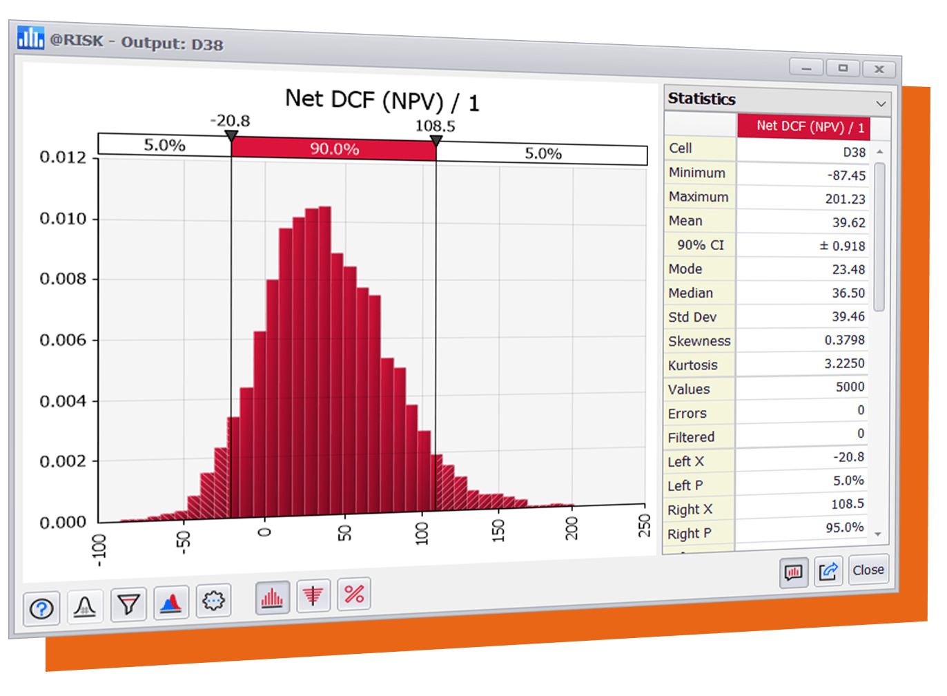
@RISK (pronounced “at risk”) software is an add-in tool for Microsoft Excel that helps you make better decisions through risk modeling and analysis. It does this using a technique known as Monte Carlo simulation. @RISK’s Monte Carlo analysis computes and tracks many different possible future scenarios in your risk model, and shows you the probability of each occurring. In this way, @RISK shows you virtually all possible outcomes for any situation. This probabilistic approach makes @RISK a powerful tool that you can use to judge which risks to take and which ones to avoid—critical insight in today’s uncertain world.
Works with Microsoft Excel
Avoid Pitfalls and Uncover Opportunities with Risk Analysis
Model Risk Factors and Protect Yourself with Contingency Planning
Communicate Risk To Others
Industries using @RISK
Energy & Utilities
Insurance & Reinsurance
Finance & Banking
Manufacturing & Consumer Goods
Construction & Engineering
Aerospace & Defense
Customer Success Stories with @RISK
Learn how @RISK has helped decision makers to improve risk and decision analysis efforts.
P&G
Robert Hunt
Associate Director for Investment Analysis, Procter & Gamble

We’ve trained well over a thousand people throughout the company on @RISK, and rely on it for our entire range of investment decisions.
Petrobras

Rafael Hartke
Financial Planning, Petrobras
@RISK helps Petrobras reduce the calculation time for projections that used to take thousands of hours to a single day. If you multiply the saved hours by staff pay rates, you can get a pretty good picture of some huge cost savings.
Post
Ulrik Mester
Risk Management Consultant at Post Danmark
The combination of our data and @RISK’s technology has given us the confidence to predict exactly what risks we face, as a result of which we do not need to pay so much for our insurance.
Lockheed Martin

Michael Watson
Integrated Program Planning — NASA Orion Multi-Purpose Crew Vehicle, Lockheed Martin
@RISK tells us the probability of making our contractual dates and highlights any areas of risk that we may not have identified. We want to know what it’s going to take to hit our milestones on time – for example, launch is extremely important.
Deloitte
Liran Blasbalg
Actuarial Analyst, Deloitte
@RISK gives us the power to perform Monte Carlo methods in a single cell in Excel. This saves us time and simplifies the spreadsheets we work in.
Merck
We love @RISK because it incorporates distribution fitting and gives us the flexibility to evaluate alternative distributions on screen.
How @RISK Is Used
@RISK enables endless applications, including these in:
- Investment Planning & Portfolio Optimization
- Cost Estimation
- Engineering Reliability
- Capital Reserves
- Oil, Gas, & Mineral Reserves

Investment Planning & Portfolio Optimization
Simulate multiple portfolio assets (such as stocks, bonds, real estate, or projects) to maximize return while minimizing risk. Calculate Value-at-Risk, or the probability of different losses on a portfolio.

Cost Estimation
Get an accurate, probabilistic estimate of materials and labor costs throughout the entire project. Understand the likelihood of going over budget under a variety of scenarios.

Engineering Reliability
Gain insight into confidence levels around the risk of equipment failure or safety violations using Six Sigma calculations. Identify areas of weakness to ensure quality results and prevent failures.

Capital Reserves
Probabilistically forecast future claims or losses in order to determine optimal reserves levels. Perform stress testing on high-impact, low-probability events.

Oil, Gas, & Mineral Reserves
Assess the likelihood of prospective sites containing oil, natural gas, metals, or other minerals. Probabilistically estimate reserves and production decline in order to make wise drilling decisions.
Investment Planning & Portfolio Optimization
Investment Planning & Portfolio Optimization
Simulate multiple portfolio assets (such as stocks, bonds, real estate, or projects) to maximize return while minimizing risk. Calculate Value-at-Risk, or the probability of different losses on a portfolio.
Cost Estimation
Cost Estimation
Get an accurate, probabilistic estimate of materials and labor costs throughout the entire project. Understand the likelihood of going over budget under a variety of scenarios.
Engineering Reliability
Engineering Reliability
Gain insight into confidence levels around the risk of equipment failure or safety violations using Six Sigma calculations. Identify areas of weakness to ensure quality results and prevent failures.
Capital Reserves
Capital Reserves
Probabilistically forecast future claims or losses in order to determine optimal reserves levels. Perform stress testing on high-impact, low-probability events.
Oil, Gas, & Mineral Reserves
Oil, Gas, & Mineral Reserves
Assess the likelihood of prospective sites containing oil, natural gas, metals, or other minerals. Probabilistically estimate reserves and production decline in order to make wise drilling decisions.
Key Features
Monte Carlo Simulation
By sampling different possible inputs, @RISK calculates thousands of possible future outcomes, and the chances they will occur. This helps you avoid likely hazards—and uncover hidden opportunities.
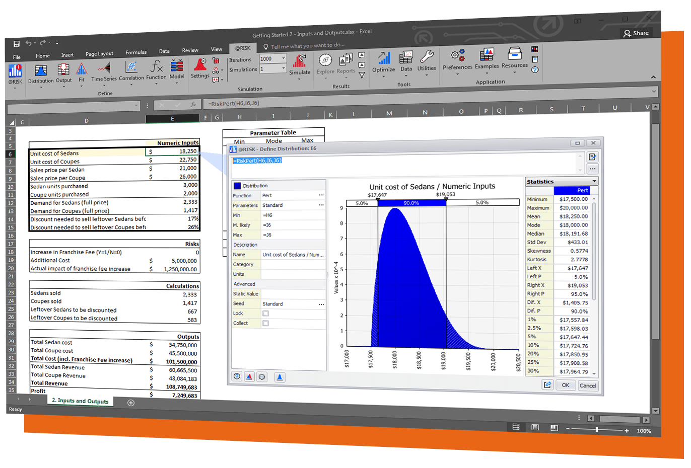
100% Excel Integration
@RISK integrates seamlessly with Excel’s function set and ribbon, letting you work in a familiar environment with results you can trust.
Sensitivity Analysis
@RISK identifies and ranks the most important factors driving your risks, so you can plan strategies—and resources—accordingly.


Graphs and Reports
@RISK offers a wide variety of customizable, exportable graphing and reporting options that let you communicate risk to all stakeholders.
Extensive Modeling Features
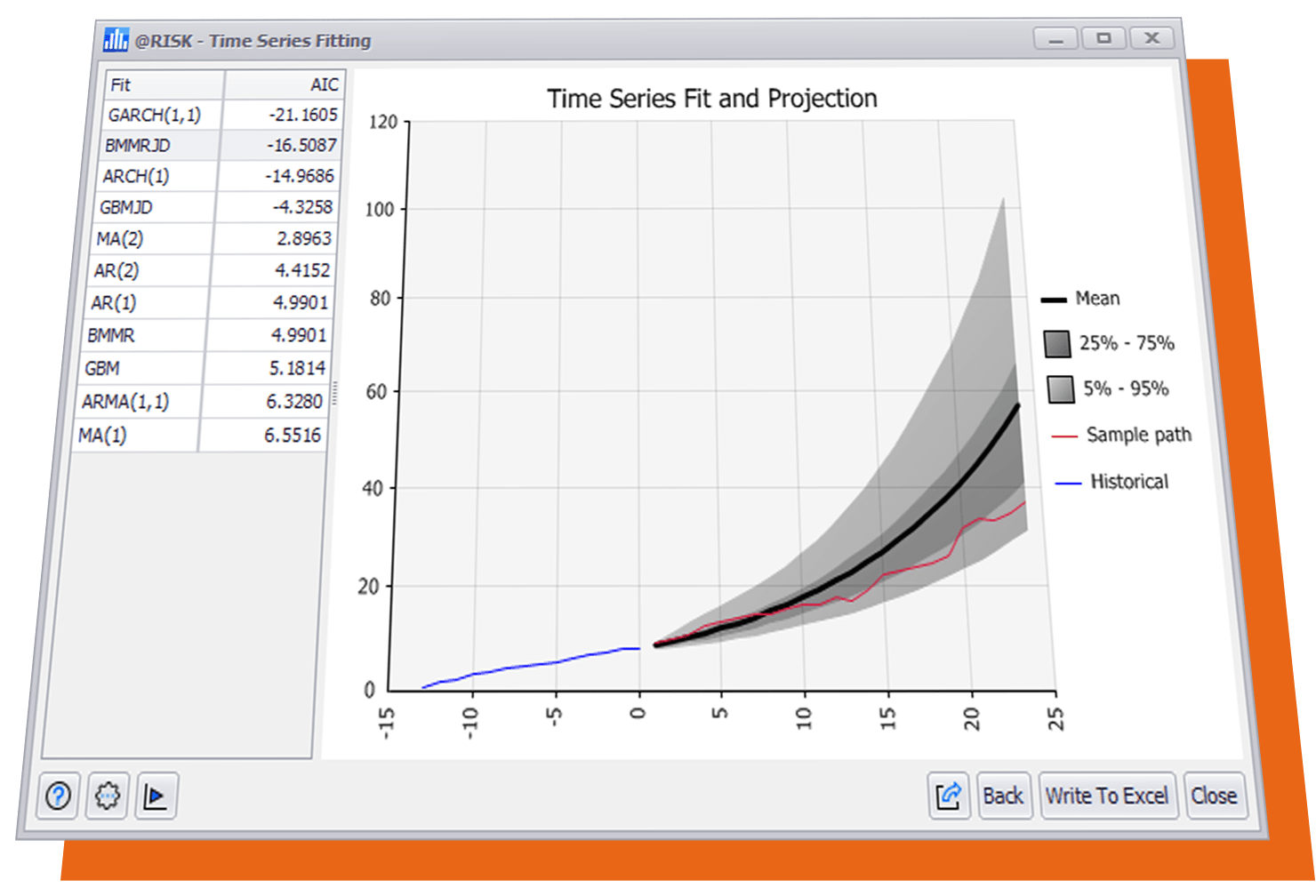
With a broad library of probability distributions, data fitting tools, and correlation modeling, @RISK lets you represent any scenario in any industry with the highest level
of accuracy.
![]()
Add Decision & Data Analysis with The DecisionTools Suite
The complete risk and decision analysis toolkit, including @RISK, PrecisionTree, TopRank, NeuralTools, StatTools, Evolver, RISKOptimizer, and ScheduleRiskAnalysis.
Additional Benefits

Your software subscription has you fully covered.
- Free upgrades when new software versions are released
- Full access to Technical Support

Technical Support is available to help with installation, operational problems, or errors.
- Included with subscription
- Phone, web, or email

Leverage the power of @RISK in your own custom application with Palisade Custom Development.
- Engage Palisade to design your solution
- Standardize your analyses and reduce learning curves
Join decision-makers around the world who
RELY ON PALISADE.
На чтение 5 мин. Просмотров 22 Опубликовано 21.05.2021

Прежде чем инвестировать, например покупать акции или облигации, нам лучше осторожно оценить стоимость, подверженную риску. Помимо профессиональных инструментов оценки, мы можем легко рассчитать стоимость, подверженную риску, по формулам в Excel. В этой статье я возьму пример для расчета стоимости, подверженной риску, в Excel, а затем сохраню книгу как шаблон Excel.
Создайте таблицу значений, подверженных риску, и сохраните в качестве шаблона
Создайте таблицу «Значение риска» и сохраните эту таблицу (выборку) только как мини-шаблон
Содержание
- Точное/статическое копирование формул без изменения ссылок на ячейки в Excel
- Рассчитать значение риска в книгу и сохраните ее как шаблон Excel.
- Сохранить диапазон как мини-шаблон (запись автотекста, оставшиеся форматы ячеек и формулы) для повторного использования в будущем
- Статьи по теме:
Точное/статическое копирование формул без изменения ссылок на ячейки в Excel
Kutools for Excel Утилита Exact Copy может помочь вам легко скопировать несколько формул без изменения ссылок на ячейки в Excel, предотвращая автоматическое обновление относительных ссылок на ячейки. 30-дневная бесплатная пробная версия полнофункциональной версии!

Вкладка «Office» Включает редактирование и просмотр с вкладками в Office и делает вашу работу намного проще …
Подробнее … Бесплатная загрузка …
Kutools for Excel решает большинство ваших проблем и увеличивает Ваша продуктивность на 80%.
- Повторное использование чего угодно: добавляйте наиболее часто используемые или сложные формулы, диаграммы и все остальное в избранное и быстро используйте их в будущем.
- Более 20 текстовых функций: извлечение числа из текстовой строки; Извлечь или удалить часть текстов; Преобразование чисел и валют в английские слова.
- Инструменты слияния: несколько книг и листов в одну; Объединить несколько ячеек/строк/столбцов без потери данных; Объедините повторяющиеся строки и суммируйте.
- Инструменты разделения: разделение данных на несколько листов в зависимости от значения; Из одной книги в несколько файлов Excel, PDF или CSV; Один столбец в несколько столбцов.
- Вставить пропуск скрытых/отфильтрованных строк; Подсчет и сумма по цвету фона; Массовая отправка персонализированных писем нескольким получателям.
- Суперфильтр: создавайте расширенные схемы фильтров и применяйте их к любым листам; Сортировать по неделе, дню, частоте и т. Д. Фильтр жирным шрифтом, формулами, комментарием …
- Более 300 мощных функций; Работает с Office 2007-2019 и 365; Поддерживает все языки; Простое развертывание на вашем предприятии или в организации.
Подробнее … Бесплатная загрузка …
 Рассчитать значение риска в книгу и сохраните ее как шаблон Excel.
 Рассчитать значение риска в книгу и сохраните ее как шаблон Excel.
 Допустим, вы собираетесь инвестировать 100 долларов, а средний доход в день составляет 0,152 . Теперь, пожалуйста, следуйте инструкциям, чтобы рассчитать, сколько вы потенциально потеряете..
Шаг 1. Создайте пустую книгу и введите заголовки строк из A1: A13, как показано на следующем снимке экрана. А затем введите свои исходные данные в эту простую таблицу.

Шаг 2. Теперь шаг за шагом вычислите величину риска:

(1) Рассчитайте минимальную доходность с уровнем уверенности 99%: в В ячейке B8 введите = НОРМ.ОБР (1-B6, B4, B5) в Excel 2010 и 2013 (или = НОРМ.ОБР (1-B6, B4, B5) в Excel 2007) и нажмите клавишу Enter key;
(2) Рассчитайте общую стоимость портфеля: в ячейке B9 введите = B3 * (B8 + 1) и нажмите клавишу Enter . ;
(3) Рассчитайте значение, подверженное риску каждый день: в ячейке B10 введите = B3-B9 и нажмите клавишу Enter ;
(4) Рассчитайте общую стоимость с риском для одного месяца: в ячейке B13 введите = B10 * SQRT (B12) и нажмите клавишу Enter .
Пока что мы выяснили, какие значения подвергаются риску каждый день и каждый месяц. Чтобы сделать таблицу удобочитаемой, мы продолжаем форматировать таблицу, выполнив следующие шаги.
 |
Формула слишком сложна для запоминания? Сохраните формулу как запись Auto Text для повторного использования одним щелчком мыши в будущем! Подробнее… Бесплатная пробная версия |
Шаг 3. Выберите диапазон A1: B1 и объедините их, нажав Главная > кнопка Объединить и центрировать > Объединить ячейки .

Затем объедините Range A2: B2, Range A7: B7, Range A11: B11 последовательно тем же способом.
Шаг 4. Удерживая клавишу Ctrl , выберите диапазон A1: B1, диапазон A2: B2, диапазон A7: B7 и диапазон A11: B11. Затем добавьте цвет выделения для этих диапазонов, нажав Home > Цвет заливки , и укажите цвет из раскрывающегося списка.

Шаг 5. Сохраните текущую книгу как Excel шаблон:
- В Excel 2013 щелкните Файл > Сохранить > Компьютер > Обзор ;
- В Excel 2007 и 2010 щелкните Файл / Office button > Сохранить .
Шаг 6. В появившемся диалоговом окне «Сохранить как» введите имя этой книги в поле Имя файла , щелкните поле Сохранить как тип и выберите Шаблон Excel (* .xltx) из раскрывающегося списка. , наконец, нажмите кнопку Сохранить .

Сохранить диапазон как мини-шаблон (запись автотекста, оставшиеся форматы ячеек и формулы) для повторного использования в будущем
Обычно Microsoft Excel сохраняет всю книгу как личный шаблон. Но иногда вам может просто потребоваться часто повторно использовать определенный выбор. По сравнению с сохранением всей книги как шаблона, Kutools для Excel предлагает обходной путь утилиты AutoText , позволяющий сохранить выбранный диапазон как запись автотекста, в которой можно сохранить форматы ячеек и формулы в этом диапазоне. вы можете повторно использовать этот диапазон одним щелчком мыши. 30-дневная полнофункциональная бесплатная пробная версия!

Статьи по теме:
Как сделать в Excel шаблон только для чтения?
Как защитить/заблокировать шаблон Excel, перезаписываемый паролем?
Как найти и изменить сохранение по умолчанию l размещение шаблонов Excel?
Как отредактировать/изменить личный шаблон в Excel?
Как изменить шаблон книги/листа по умолчанию в Excel?
In portfolio management, Value-at-Risk (VaR) is a popular metric to quantitatively assess the risk of our holdings.
Originally invented by banks to give some sense to how much lost could be reasonably anticipated across different business, it gained traction in the risk management world and soon become a well-known method to measuring risk and helping traders/portfolio managers to view their portfolio in a different fashion.
Today let’s learn about what is VaR, and how we can compute it in Excel.
You may also be interested in 2021 New Year Resolution List for Excel.
Workbook
What is Value-at-Risk (VaR)?
Value-at-Risk (VaR) is, in essence, the X-percentile of the projected Profit-and-loss (PnL) for our portfolio, over a given time horizon. In plain words, if VaR is $100, it tells you that if we are unlucky tomorrow, we expect to lose at a maximum of $100 with X% chance/confidence.
Let’s think about it in a non-financial example. Suppose you have 99 students in a Mathematics class, taking the same test tomorrow. Based on the result of the last test they’ve taken, you obtained a projection of how the class will perform in the coming test.
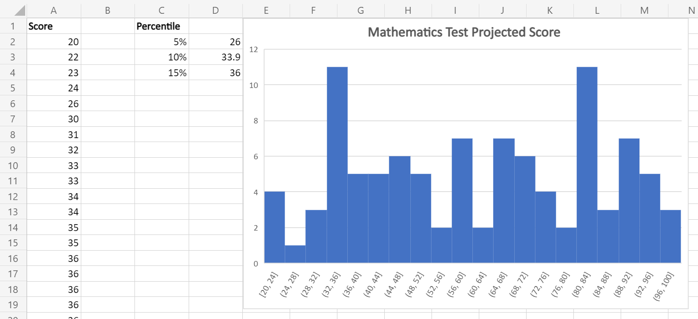
With the data in our example workbook, we found that the 5th percentile of the score is at 26, which is basically the 5th-lowest score achieved by the class (cell A6). Therefore, we can loosely say that the 5% Value-at-Risk for the class is 26 in the upcoming test, i.e. we have 5% confidence that the lowest score achieved by all students is 26.
You may also be interested in Binomial Option Pricing (Excel formula).
Why do we use Value-at-Risk (VaR)?
Now let’s turn our attention to portfolios of financial instruments. Instead of the score of students, now we look to project the Profit-and-Loss (PnL) of our portfolio, and compute a Value-at-Risk (VaR) based on that.
There are actually good reason to look at Value-at-Risk (VaR), on top of usual metrics like expected return/portfolio standard deviation. VaR is actually a metric to look at heavy-tail events (or black-swan events).

Heavy-tail (or black-swan) events are rare events that have severe consequence. For example, people generally think the stock market would not drop by more than 5% a day, so “Market dropping by more than 5%” is a black-swan event.
While metrics like expected return/portfolio standard deviation give investor a sense of the characteristics of their portfolio, they do not tell you what could happen if you have a really bad day. And VaR is a good metric to tell you that, if you have a really bad day, what is the loss to be expected.
For large investor, heavy-tail events are risks to be managed, and hence heavy-tail metrics like VaR has grown in prominence for risk management.
With this in mind, our problem becomes:
- How do we present VaR figures?
- How do we come up with the statistical distribution of the PnL (i.e. the chances of achieving different PnL levels)?
Let’s go through one-by-one in the following section.
You may also be interested in How to Compute IRR in Excel (Basic to Advanced).
How do we present Value-at-Risk (VaR)?
In practice, Value-at-Risk (VaR) often comes in different flavors, and it is important for us to understand how to read into the VaR figures provided.
Confidence Level
VaR is always presented in the manner “X%-VaR“, and we specify the confidence level (i.e. X%) related to a specific VaR. For example, a 95%-VaR would correspond to the 5th-percentile of the PnL distribution, 99%-VaR to the 1st-percentile of the PnL distribution.
There is no one-shoe-fit-all rule that dictates what is the confidence level to use, but practitioners generally quotes multiple confidence level at once (e.g. 95%, 97.5%, 99%) to give a better sense for how heavy-tail events would impact the portfolio.
Time Horizon
VaR is also commonly presented as a “X-day VaR“, although sometimes it is implicitly a 1-day VaR measure. When speaking of the PnL distribution, depending on the frequency of the data (e.g. daily/weekly/monthly), VaR of different time horizon could be calculated.
Majority of the VaR measures in practice is a 1-day metric, as a typical assumption is that risks are reviewed on a daily basis, but longer horizon metrics are often useful as well.
Absolute vs Relative
Absolute and Relative VaR differs in whether you want to benchmark against the expected return.
For example, suppose the 5th percentile of your PnL distribution is -$10, and your expected return (i.e. mean of PnL distribution) is +$2. Your Absolute 95%-VaR would be -$10 (the total loss expected), and your Relative 95%-VaR would be -$8 (a relative figure to the expected return).
You may also be interested in How to Generate Random Variables in Excel.
How do we come up with the statistical distribution?
After we discussed on what are the flavors for Value-at-Risk (VaR), we look at a more fundamental question – how do we come up with the distribution of potential Profit-and-Loss (PnL) in the first place?
Ultimately, the computed VaR depends on your selected PnL distribution: if you select a distribution that there is a high chance of losing (positively skewed), chances are, your VaR computed will be larger than if you have picked a distribution that is more symmetrical.
There are mainly 2 ways which we’ll illustrate with the help of Excel:
- Historical approach
- Parametric approach
Historical Approach
As the name suggest, in historical approach, you compute the VaR based on what is available in the past.
In essence, based on the specific portfolio composition, we obtain the daily PnL data, sort them in ascending order, and find the relevant (1-X)-th percentile that translates to our X%-VaR.
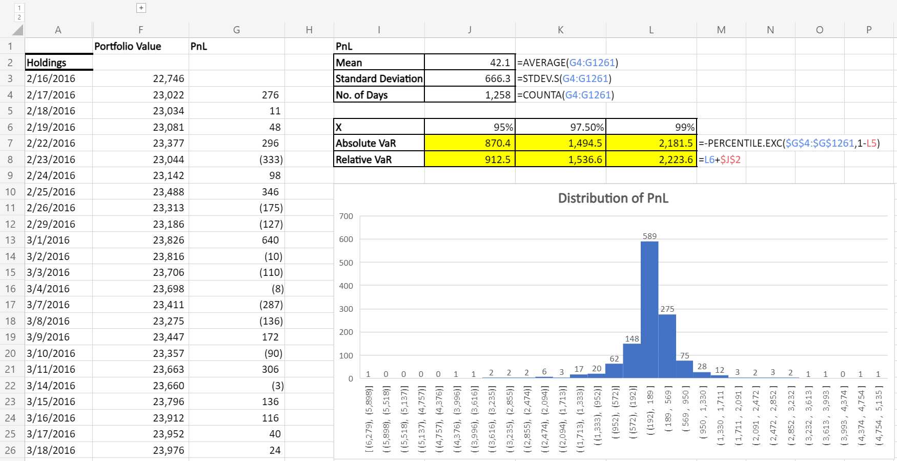
From the Sample Workbook, you’ll find an example where we have a portfolio with 4 stocks. With Yahoo Finance stock price data, we compute the day-on-day change as our PnL distribution.
Based on the calculation, we found that the 1-day 95%-VaR is $870.4, which means on a given day, we expect that the maximum loss is $870.4 with 5% confidence. Similarly we have the 97.5%-VaR and 99%-VaR for side-by-side comparison.
As you’ve guessed, there are several limitation of using a historical approach:
- The computed VaR is heavily influenced by the timeframe you’ve selected.
- Past performance of the portfolio does not necessarily link closely to future performance
- Most importantly, sampling of the negative outliers (i.e. days with large loss) may be biased as we usually have too few observations.
With that in mind, we introduce the alternative approach: the parametric approach.
You may also be interested in Black-Scholes Option Pricing (Excel formula).
Parametric Approach
The parametric approach is a fancy way to say that we make some statistical assumption with the PnL distribution.
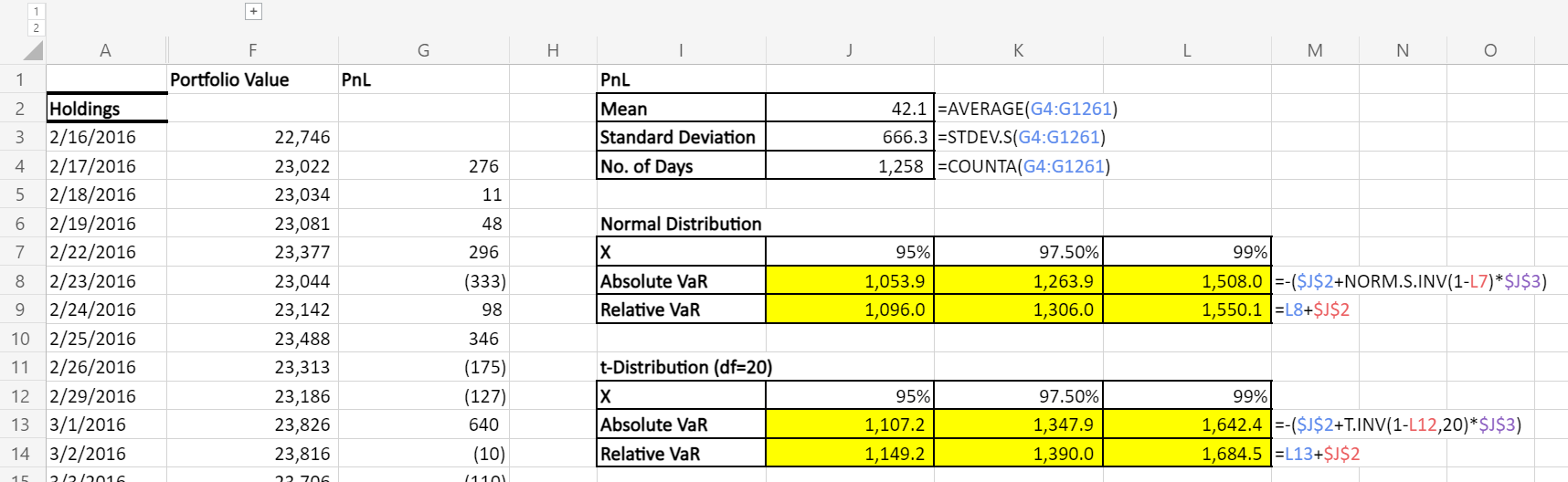
For example, in our sample workbook, we’ve presented VaR computed from 2 commonly-used parametric distribution: the Normal distribution and the t-distribution.
In the Parametric Approach, we only need to estimate for a couple of parameters (e.g. mean and standard deviation) of the PnL distribution, and apply these parameter to find the expected percentile.
Notice how the VaR computed for t-distribution is larger than the normal distribution, which is due to the fact that t-distribution has heavier tails than the normal distribution. Heavier tail means that there are more chances for outliers (negative outcome in our case).
Comparing what we computed in parametric vs historical approach, while parametric approach seems more prudent than the historical approach for 95%-VaR (1,053.9 vs 870.4, larger means more prudent), for 99%-VaR (1,508.0 vs 2,181.5) the opposite is true.
In this case, we’ll need to re-evaluate whether our choice of parametric PnL distribution (e.g. Normal/t) is representative of the actual PnL distribution, and see if we need to find a more heavy-tailed distribution.
You may also be interested in How to Name Multiple Single Cells in Excel.
Bottomline
Value-at-Risk (VaR) is an important metric in risk management, giving investors/traders the sense of how heavy-tail/black-swan events would impact the portfolio of financial instruments we hold.
There are numerous ways to how VaR can be computed and presented, but we should always compare and contrast VaR computed with different approach and understand what it means for our modelling and how it could be representative of our risks.
You may be interested in How to use REPT functions to the Most.
Hungry for more useful Excel tips like this? Subscribe to our newsletter to make sure you won’t miss out on any of our posts and get exclusive Excel tips!
5 mins read
In this post, we will calculate Value at Risk in EXCEL using the VaR Historical Simulation approach.
1. What is Value at Risk?
Perhaps the simplest and common concept you are likely to see when it comes to financial risk management is Value at Risk or VaR for short. It represents an educated estimate for:
a) How bad can prices get when they really get bad? or
b) What is the most that you can lose on a really bad day on account of price changes? or
c) What is the worst that can happen when the market hits free fall?
While VaR has received a great deal of negative coverage post 2008, before we discuss issues, it would be useful to first determine how to calculate Value at Risk.
There are three methods for calculating Value at Risk. Variance covariance (VCV), Historical Simulation and Monte Carlo Simulation. In this post, we will start off with a data series for the USD-EUR Foreign currency exchange rate. Then see what the Value at Risk measure can tell us about the likely (most common) and the worst case (extreme) movement for this exchange rate.
We will calculate Value at Risk using the Historical Simulation approach in EXCEL.
2. Guide to the Value at Risk Historical Simulation Approach
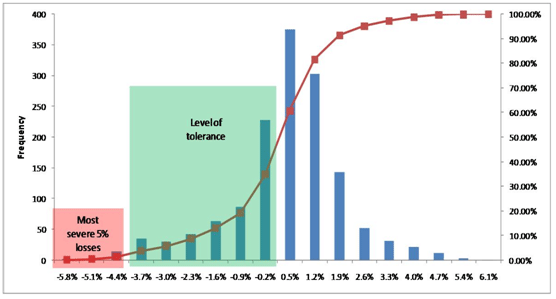
For example, take a look at the following EXCEL histogram.
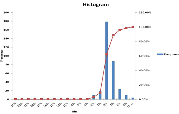
This histogram is calculated using a series of daily price changes for a given financial security. Within risk terms, we call daily price changes, daily returns, and these returns could be positive or negative.
The histogram above takes a daily return series, sorts the series and then slots each return in a given return bucket.
a. Step 1 – Calculate daily returns
We will first calculate a table of daily returns from the daily USD-EUR exchange rates daily exchange rate series. Each return is calculated by the application of LN(P1/P0) where LN is the natural log function in EXCEL, P1 is the new exchange rate, P0 is the old exchange rate. This is approximately equal to the daily % price change in the underlying exchange rate.
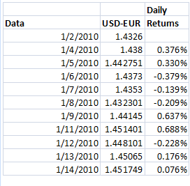
We will take this return series and use it to calculate a histogram similar to the one above.
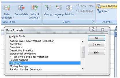
b. Step 2 – Set up & run EXCEL’s Data Analysis Histogram tool
You can find the Histogram tool under the Data Analysis tab in Excel. If for some reason you don’t see a data analysis tab in your version of EXCEL, to enable the tab do the following:
- Go to EXCEL Options
- Choose Addins, and
- Add the Data Analysis Addin.
To generate the Histogram select the daily return series by calculating the percentage change in prices from one day to the next. Use that return series as your input range.
Opt for New worksheet ply, cumulative percentage and chart output (see below) to see a graphical representation of the Histogram as well as a supporting table.
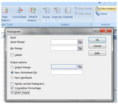
When you press ok, EXCEL will create a new tab for you and show the histogram that you see below.

c. Step 3 – Interpreting the results of the histogram
As a risk professional our focus is on the downside which in the histogram below is marked at -2.77%. The upside is about 1.99+%.
i. Worst case loss?
So if I asked you what is the worst that can happen, you can easily tell me that my worst scenario based on historical returns as shown by the above histogram is a loss of over -2.77% (the extreme left corner on the bottom) if I am long (bought) Euro or a loss of 1.99% if I am short (sold) Euro versus the US dollar.
ii. Time period? Odds?
Your next two questions should be, over what time and with what odds?
The returns are calculated on a daily basis hence the answer to the first question is over anyone given trading day.
The second answer requires a bit of work. There are approximately 300 days (frequency count) in the graph above. Your worst case loss is a once in 300 day event. The probability of you seeing a loss greater than this number is 1/300 or 0.33%.
Fortunately, the EXCEL histogram output worksheet already has a table with these probabilities and numbers in it.
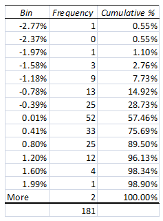
iii. Putting it together
If you put it together there is only a .55% chance that you or I will see a worst case loss of over -2.77% on any given trading day if you bought Euros and a 1.1% chance that you will see a loss of over 1.99% if you have sold Euros.
Congratulations. By adding a holding period (a given trading day) and a probability (0.55% / 1.1%) you have converted your simple what is the worst that can happen statement into a value at risk estimate.
Typically Value at Risk (VaR) is expressed in dollar terms. However, since here we only had percentile returns to work with we have expressed it in percentage terms.
Conceptually Value at Risk represents the projected level of losses a trading desk needs to protect itself against under extreme conditions. It is used as a proxy for the amount of capital required to support such losses.
3. Alternative Value at Risk methods
The approach that we have just used to calculate Value at Risk is also known as the VaR Historical Simulation approach.
You can also calculate Value at Risk using the Variance covariance (VCV) approach or using the Monte Carlo simulation approach.
The VaR Historical simulation approach works with the actual distribution of results (the price and return series), the VCV approach assumes that returns are normally distributed (it imposes the normal distribution) while the Monte Carlo Simulation technique uses a generator function to first simulate a series of prices and then applies the same process we have used above for Historical simulation.
a. Using the right models
As is the case with practitioners, as we solve new problems (sometimes creating other more difficult to solve problems), we build up an inventory of biases and prejudices.
I greatly like Monte Carlo simulation as a tool for dissecting structures and testing pricing and hedging strategies. However, I hate it (Monte Carlo simulation) when it comes to modeling risk. I realize that the Historical Simulation approach has many significant limitations. But over the years, it’s the only approach that has shown some sense of stability. As Nassim Taleb puts it, history is not going to repeat itself, you are not going to be hit by your last worst loss and the next big wave that will wipe you out will not come from where you expect it.
My respect for historical simulation grew when we started modeling Value at Risk for cross currency swaps. Two separate currencies, two separate interest rates, two separate term structures and about a thousand assumptions in between. I would look at the end number our Monte Carlo simulator would throw out in amazement and wonder how could any rationale being put any reliance on something that is literally stitched together by chewing gum and baling wire.
While Historical simulations had its own issues, at least it reduced the assumption set and the usage of historical price data set across currency pairs, rates, term structures and markets made it a lot easier to explain to traders. Traders understand and respect price and price histories. They question assumptions. A model that uses raw prices unfettered by drivers and assumptions for a trader is infinitely superior to a model with more assumptions than equations.
For additional examples and instruction please see the following lessons:
- Calculating value at risk case study and example
- Portfolio Var – Shortcut approach without VCV
By Chainika Thakar
What is the most I can lose on an investment? This is the question every investor who has invested asks at some point in time. Value at Risk (VaR) tries to provide an answer since it is the measurement of the maximum expected loss a portfolio bears.
We will understand and perform VaR calculation in Excel and Python using the Historical Method and Variance-Covariance approach, along with examples with this blog that covers:
- What is VaR?
- Why use VaR?
- Essential points to know while using VaR
- How is VaR calculated in Excel?
- VaR calculation using Variance-Covariance approach
- VaR calculation using the Historical Simulation approach
What is VaR?
Value at Risk or VaR is the measurement of the worst expected loss over a specified period under the usual market conditions. The VaR is measured using ‘confidence levels’ which lie in the range of 90% to 99% such as 90%, 95%, or 99%. The holding period of the financial instrument may vary from a day to a year.
In other words, VaR is a measure of market risk. It is the measure of maximum loss that can occur with a certain confidence interval over a given period of time. Using VaR, financial institutions can determine the sufficient capital reserves they need to cover losses. Also, VaR helps determine whether higher than acceptable risk holdings need to be reduced.
According to Philippe Jorion,
“VaR measures the worst expected loss over a given horizon under normal market conditions at a given confidence level”.
Also, according to one of the studies ⁽¹⁾, it was concluded that VaR does not provide any certainty but rather expectation of outcomes based on certain assumptions.
Download Var Models in Excel & Python
Login to Download
Example
Lets us understand VaR with an example.
Suppose, an analyst says that the 1-day VaR of a portfolio is 1 million dollars, with a 95% confidence level.
- It implies there is a 95% chance that the maximum losses will not exceed 1 million dollars in a single day.
- In other words, there is only a 5% chance that the portfolio losses on a particular day will be greater than 1 million dollars. Learn quantitative portfolio management in detail in the Quantra course.
Why use VaR?
Now, let us find out why one uses VaR or Value at Risk for measuring the expected loss. A trader utilises VaR for the following reasons:
- Understanding the Value at Risk result is easy
- Applicable to all asset types
- Universally utilised
Understanding the result of Value at Risk is easy
Value at Risk represents the extent of risk a trader bears for investing in a portfolio in a single figure. For instance, the Value at Risk is between 90% and 99% which makes it easy to interpret the level of risk.
Applicable to all asset types
Vale at Risk can be easily applied to all asset types, namely, bonds, shares, currencies, derivatives, etc. Also, Value at Risk is utilised by all kinds of financial institutions and banks in order to assess the profitability over risk borne for trading a portfolio or asset. Learn Financial Time Series Analysis for Trading in detail in the Quantra course.
Universally utilised
Value at Risk is an accepted standard for basing buying, selling and all trade-related activities. Hence, you can use it anywhere across the globe.
Download Var Models in Excel & Python
Login to Download
Essential points to know while using VaR
There are a couple of essential points that a trader must know while using VaR as the measurement of risk against investment in a portfolio or financial instrument. These points are:
1. VaR is difficult to calculate for portfolios with a diversity of assets (such as cash, currency, stocks etc.) or a greater number of assets
Calculating Value at Risk for a portfolio needs one to calculate the risk and return of each asset. But, along with the risk-return calculation, the correlations between the assets are also to be calculated. Hence, the more the number or diversity of assets in a portfolio, the more difficult it is to calculate VaR.
2. Different methods or approaches lead to varying results
When different approaches to calculating VaR lead to different results for the same portfolio or the financial instrument, it implies the return distribution is not normal.
How is VaR calculated in Excel?
There are two well-known methods that are used for VaR calculation.
In this blog, we will discuss the following:
- Variance-covariance approach
- Historical simulation approach
Let’s start with the Variance-Covariance approach.
The Variance-covariance is a parametric method which assumes that the returns are normally distributed. In this method,
- We first calculate the mean and standard deviation of the returns
- According to the assumption, for 95% confidence level, VaR is calculated as a mean -1.65 * standard deviation
- Also, as per the assumption, for 99% confidence level, VaR is calculated as mean -2.33* standard deviation
Please note that the abovementioned figures are on the basis of a subjective assumption ⁽²⁾.
Moving on, the steps for VaR calculation using the Historical simulation approach are as follows:
- Similar to the variance-covariance approach, first we calculate the returns of the stock Returns = Today’s Price — Yesterday’s Price / Yesterday’s Price
- Sort the returns from worst to best.
- Next, we calculate the total count of the returns.
- The VaR(90) is the sorted return corresponding to 10% of the total count.
- Similarly, the VaR(95) and VaR(99) is the sorted return corresponding to the 5% and 1% of the total count respectively.
Download Var Models in Excel & Python
Login to Download
VaR calculation using Variance-Covariance approach
Now, we will find out the calculation if Variance-Covariance approach using Python.
Output:

Now, we will use confidence level, mean and standard deviation in the Python code.
Output:
Confidence Level      Value at Risk
------------------  ---------------
95%                      -0.0319445
99%                      -0.0457278
The values above imply the confidence level of the particular “value” that is at a risk of being lost.
Hence, there is a 95% of confidence that the loss of value may be -0.0319445 and not more and there is 99% confidence that the loss will go to -0.0457278 and not beyond. Since all the values at risk are in negative, the probability is higher that the portfolio will return more than invested amount.
Download Var Models in Excel & Python
Login to Download
VaR calculation using the Historical Simulation approach
Now, let us calculate the VaR using the historical simulation approach.
Output:

Output:
Confidence Level      Value at Risk
------------------  ---------------
90%                      -0.0219604
95%                      -0.0288828
99%                      -0.0527869
The above values imply the confidence level of the particular “value” that is at a risk of being lost. Hence, the confidence rate is 90% that the loss may be -0.0219604 and not above.
Similarly, there is a 95% of confidence that the loss of value may be -0.0288828 and nor beyond and there is 99% confidence that the loss will go to -0.0527869 but not further than that. Since all the values at risk are in negative, there is a higher probability of the portfolio returning more than invested amount.
From the calculation above, you can see there is a substantial difference in the percentage of value-at-risk calculated from historical simulation and variance-covariance approach. This tells us that the return distribution is not normal.
Although both the approaches return negative values (indicating more probability of higher returns), there is still a difference in the figures of values which implies that the distribution is not normal.
Recommended reads:
- Covariance Matrix and Portfolio Variance: Calculation and Analysis
- Covariance and Correlation: Intro, Formula, Calculation, and More
- Portfolio Analysis: Calculating Risk and Returns, Strategies and More
Conclusion
In this blog, we covered the two integral ways of using Value at Risk in both Excel and Python. A trader can use VaR for measuring the risk of trading if the essential points of using the same are kept in mind.
If you wish to learn more about VaR, you can gain essential skills required for different quant trading desk roles such as trader, analyst, and developer, you too can do it. This learning track which is algorithmic trading for everyone by Quantra is perfect for traders and quants who want to learn and use Python in trading. Enroll now!
File in the download
- VaR calculation in Excel
Login to Download
Note: The original post has been revamped on 9th December 2023 for accuracy, and recentness.
Disclaimer: All investments and trading in the stock market involve risk. Any decision to place trades in the financial markets, including trading in stock or options or other financial instruments is a personal decision that should only be made after thorough research, including a personal risk and financial assessment and the engagement of professional assistance to the extent you believe necessary. The trading strategies or related information mentioned in this article is for informational purposes only.
