Arrow button in excel

Pressing an arrow key while SCROLL LOCK is on will scroll one row up or down or one column left or right.
Use the arrow keys to move through a worksheet.

To scroll	Do this
One window left or right	Press SCROLL LOCK, and then hold down CTRL while you press the LEFT ARROW or RIGHT ARROW key.

Why do my arrow keys not work in Excel?

One of the common reasons why the arrow keys don’t work in Excel is because you’ve enabled the scroll lock feature on your computer. For as long as it remains enabled, the keys won’t do what they’re supposed to do.Simply press the scroll lock button on your keyboard and the lock will be disabled.

How do I unlock scroll lock in Excel?

Click Change PC Settings. Select Ease of Access > Keyboard. Click the On Screen Keyboard slider button to turn it on. When the on-screen keyboard appears on your screen, click the ScrLk button.

How do I turn off cursor lock in Excel?

To turn off scroll lock, execute the following step(s).

1. Press the Scroll Lock key (Scroll Lock or ScrLk) on your keyboard.
2. Click Start > Settings > Ease of Access > Keyboard > Use the On-Screen Keyboard (or press the Windows logo key + CTRL + O).
3. Click the ScrLk button.

Where is my Scroll Lock key?

Sometimes abbreviated as ScLk, ScrLk, or Slk, the Scroll Lock key is found on a computer keyboard, often located close to the pause key. The Scroll Lock key was initially intended to be used in conjunction with the arrow keys to scroll through the contents of a text box.

How do I move the cursor in Excel?

Press the Home key to move to cell A4. Pressing Home moves the cursor to the beginning of the current row, which in this case, is row 4. Press the Page Down key.
In This Article.

Press This . . .	To Move . . .
Shift+Tab	One cell to the left

What is shortcut for Scroll Lock?

The official Microsoft shortcut for Scroll Lock is Shift + F14.

How do you unlock the cursor on a laptop?

How to Unfreeze a Laptop Mouse

1. Press and hold down the “FN” key, which is located between the Ctrl and Alt keys on your laptop keyboard. Video of the Day.
2. Tap the “F7,” “F8” or “F9” key at the top of your keyboard. Release the “FN” button.
3. Drag your fingertip across the touchpad to test if it is working.

How do you unlock the arrow keys on a laptop?

On a Windows computer, to toggle scroll lock on and off, press the Scroll Lock key. On most keyboards, it’s located in the control keys section of the keyboard, above the arrow keys or right of the function keys. On a Mac computer, to toggle scroll lock on and off, press the F14 or the Shift + F14 key combination.

How do I move the cursor in Excel using the keyboard?

Move around a workbook using the keyboard

1. To move to the next cell, press the Arrow Keys.
2. To move to the next cell to the right, press TAB.
3. To move to the next cell to the left, press SHIFT + TAB.
4. To move to the edge of a data region, press CONTROL + Arrow Keys.
5. To move to the first cell in the row, press HOME.

Why my cursor is not moving in Excel?

Windows – Turn off the Scroll Lock feature by pressing the Shift-Scroll Lock (ScrLk) keys. Alternately, use the On-Screen Keyboard and click the ScrLk button in the lower right.

How do I get my normal cursor back?

Step 1: Navigate to the Mouse Properties window as we did earlier. Step 2: Select the Pointers tab. Step 3: To select a custom cursor for the highlighted individual icon, click Browse. Step 4: That will open the default Cursors folder, where hundreds of different cursor options are available.

What do I do if my cursor is not moving?

Look for a Touchpad switch on the keyboard
The first thing to do is check for any button on your keyboard which has an icon that looks like a touchpad with a line through it. Press it and see if the cursor starts moving again. If not, check your row of function keys at the top of the keyboard.

What to do if cursor is not working?

Here’s how:

1. On your keyboard, hold down the Fn key and press the touchpad key (or F7, F8, F9, F5, depending on the laptop brand you’re using).
2. Move your mouse and check if the mouse frozen on laptop issue has been fixed. If yes, then great! But if the problem persists, move on to Fix 3, below.

How do I unlock arrow keys in Excel Windows 10?

Case Study 1: For Windows 10 (Scroll Lock Excel)

1. Step 1: Click Start >Settings>Ease of Access>Keyboard.
2. Step 2: Click the On-Screen Keyboard button to turn it on.
3. Step 3: When the on-screen keyboard appears on your screen, click the “ScrLk” button.

What key moves the cursor?

arrow keys help to move the cursor on the screen of a computer.

Which key is used to move the cursor to the right?

Press w (“word”) to move the cursor to the right one word at a time. Press b (“back”) to move the cursor to the left one word at a time. Press W or B to move the cursor past the adjacent punctuation to the next or previous blank space. Press e (“end”) to move the cursor to the last character of the current word.

Why is my cursor moving with arrow keys?

If the user has not enabled Mouse Keys, then the mouse cursor starts moving with the direction keys of the keyboard mainly either because of a software glitch in Microsoft Paint or because of the in-built settings. Also, third-party applications like Neat Mouse can cause this type of behaviour for the cursor.

What’s this keyborad shortcut to do?

• Move one cell up, down, left, or right in a worksheet.
• Scrolls left, right, up, or down one cell.
• Move selected shapes up, down, left, or right (0.5px each move).
• ← or → arrow key selects the tab to the left or right when the ribbon is selected. When a submenu is open or selected, these arrow keys switch between the main menu and the submenu. When a ribbon tab is selected, these keys navigate the tab buttons.
• ↓ or ↑ arrow key selects the next or previous command when a menu or submenu is open. When a ribbon tab is selected, these keys navigate up or down the tab group.
• In a dialog, arrow keys move between options in an open drop-down list, or between options in a group of options.

More:

• ↓ or Alt+↓ opens a selected drop-down list.
• Ctrl+Arrow key moves to the edge of the current data region in a worksheet.
• Shift+Arrow key extends the selection of cells by one cell.
• Ctrl+Shift+Arrow key extends the selection of cells to the last nonblank cell in the same column or row as the active cell, or if the next cell is blank, extends the selection to the next nonblank cell.

Why You Should be Using Keyboard Shortcuts

1. Efficiency: Many users find that using keyboard shortcuts for Excel helps them work more efficiently. In other words, using keyboard shortcuts could save you a lot of time, it’s easier and gets your job done faster.
2. Multitasking: Be a master at multitasking when needed. For example, when you are coding, writing reports or doing some research, it’s common to end up juggling dozens of open tabs at once. Knowing the right shortcuts allows you to easily find the tab you need in less than a second.
3. Health benefits: Cutting down on your mouse usage by using keyboard shortcuts can help reduce the risks of RSI (Repetitive Syndrome Injury). By alternating mouse and keyboard usage you can reduce the risks of R.S.I. and reduce the fatigue your wrists and fingers.
4. Complementarity: You can combine the advantages of using the keyboard with those of using the mouse.
5. Precision: When you have a job that requires precision it is advisable that you use the keyboard.

Home / Excel Basics / Insert an Arrow in a Cell in Excel

Sometimes you need some symbols to use as a quick indicator within the Excel data and for this Excel has the option to insert an arrow and many other predefined symbols or shapes within the cells.

It is a quick process with only three or four steps to insert an arrow and other symbols in Excel.

Insert an Arrow in a cell as Symbol

1. First, select and edit the cell in which you want to insert an arrow as a symbol.
2. After that go to the “Insert” tab and then click on the “Symbols” icon on the ribbon and click on the “Symbol” option.
   
3. Once you click on the “Symbol” option, it will display a pop-up with multiple symbols options to choose from.
4. Now, select an arrow that you want to insert in the selected cell and click “Insert” and then “close”.
   
5. At this point, the selected arrow is inserted in the selected cell.
   

You can select and insert multiple arrows and symbol options in one cell, but you cannot insert the symbol in more than one cell in one go.

For this, you need to insert the symbol in a single cell and then can copy that symbol from the cell and paste it to multiple cells.

1. First, go to the “Insert” tab and then click on the “Illustrations” icon on the ribbon and click on the “Shapes” option.
   
2. Once you click on the “Shapes” option, it will display multiple shape types with multiple arrow shapes.
   
3. Now click an arrow, which you want to insert and with the help of the mouse cursor go anywhere in the sheet and click hold the mouse button and drag the arrow where it is required.
4. At this point, the selected arrow as a shape is inserted in the cell.
5. From the “shape Format” tab under the “Shape Styles” group, you can change the arrow’s color, size, and effect.
   

Insert Upward and Downward Arrow Using Conditional Formatting

1. First, select the cells where you need to insert the upward and downward arrows and then click on the “Conditional Formatting” icon in the ribbon.
   
2. Now select the “Icon Sets” and then click on the arrows you want to insert.
3. At this point, upward and downward  “Red, Yellow, and Green” arrows are inserted in the selected cells.
   

Insert an Arrow Using the Wingdings 3 Font

To insert an arrow using the wingdings 3 font, you need to have a list of characters that can be converted to an arrow and other symbols within Excel.

1. First, enter the character in the cell where you need to insert an arrow.
   
2. After that, go to the “Font” group in the ribbon and click on the font drop-down icon and select the “Wingdings 3” font.
   
3. At this point, your character is converted to an arrow symbol based on the character which you had entered in the cell.
   

When you’re working on an Excel spreadsheet, the best way to move between cells is to use the arrow keys on your keyboard. With these keys available for each direction, you can easily go from one cell to another with a single key-press.

Sometimes, it happens that these arrow keys do not work in Excel. In some cases, they even take you to the next worksheet instead of moving to the next cell in the line. If you’re frustrated by this behavior, you’ll probably want to find out how to fix it.

Fixing the arrow keys not working in Excel issue is actually easier than you think. In most cases, you’re just a single keystroke away from getting the keys to do what they should be doing.

Also, be sure to watch our YouTube video where we go through the different solutions mentioned in this article in a short and compact video.

HOW TO FIX ARROW KEYS NOT WORKING: In Excel

Disable Scroll Lock

One of the common reasons why the arrow keys don’t work in Excel is because you’ve enabled the scroll lock feature on your computer. For as long as it remains enabled, the keys won’t do what they’re supposed to do.

If you take a look at your keyboard, you’ll find that the light for the scroll lock button is turned on. It indicates the lock is enabled, and you need to turn it off to activate the arrow keys.

If the above reason is why the arrow keys are not working in Excel on your computer, fixing it is just a matter of a key press.

• Simply press the scroll lock button on your keyboard and the lock will be disabled.

• You should find that the scroll lock light is no longer on on your keyboard.

Use The On-Screen Keyboard To Turn Off Scroll Lock

If you’re using a modern computer with an equally modern keyboard, you may notice that there’s no scroll lock button on your keyboard. It’s because most modern equipment has done away with that button thinking most users just won’t use it.

However, Windows has an on-screen keyboard available to help you use the keys that don’t exist on your actual keyboard. You can also use it on the occasions when your real keyboard gets broken or just won’t function normally.

You can use this on-screen keyboard to turn the scroll lock off.

• Open the Start Menu and search for and launch On-Screen Keyboard. It should open.

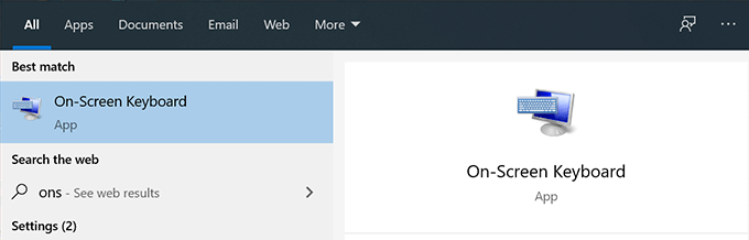
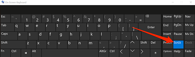
• On the right-hand side of the keyboard, you’ll find all the lock keys. There’ll be a key named ScrLk which should help you enable and disable scroll lock on your PC. Click on it and it’ll disable the scroll lock if it was enabled before.

Fix Arrow Keys Not Working With An AppleScript On Mac

Mac keyboards usually don’t have the scroll lock button on them and so disabling the feature is quite a task for you if you’re a Mac user. However, there’s a workaround that uses an AppleScript to let you fix the issue in Excel on your Mac.

The workaround creates an AppleScript and runs it when you use Excel on your machine. It then does what it needs to do to get the arrow keys to work in the Excel program.

Creating an AppleScript and executing it may sound a bit technical but it’s actually pretty easy to do.

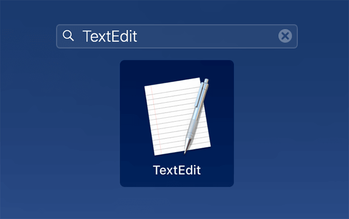
• Click on Launchpad, search for TextEdit, and open it.

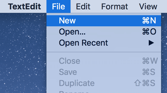
• Click on the File menu at the top and select New to create a new document.

• Copy the following code and paste it into your document.

set returnedItems to (display dialog "Press OK to send scroll lock keypress to Microsoft Excel or press Quit" with title "Excel Scroll-lock Fix" buttons {"Quit", "OK"} default button 2)
set buttonPressed to the button returned of returnedItems
if buttonPressed is "OK" then
tell application "Microsoft Excel"
activate
end tell
tell application "System Events"
key code 107 using {shift down}
end tell
activate
display dialog "Scroll Lock key sent to Microsoft Excel" with title "Mac Excel Scroll-lock Fix" buttons {"OK"}



  


                       
  



end if

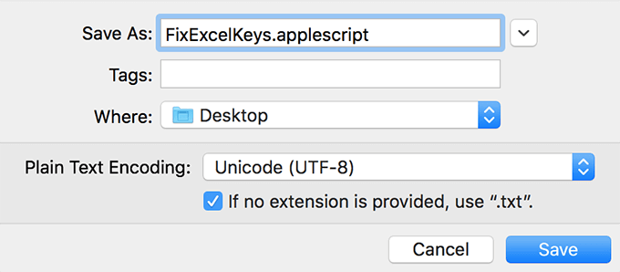
• Press the Command + S keys to save the file.
• Enter FixExcelKeys.applescript as the name of the file and save it.

• Launch your spreadsheet in Excel.
• Double-click on the newly created AppleScript file and it should fix the issue for you.

Enable Sticky Keys

In most cases, the above methods should fix the arrow keys not working in Excel issue for you. However, if you didn’t have any luck with them, you might want to try a few more and see if they help you resolve the problem.

One of these methods is to enable the sticky keys feature on your Windows computer. While it isn’t directly related to Excel or arrow keys, it’s worth toggling it to see if it fixes the issue for you.

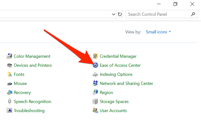
• Search for Control Panel using Cortana search and launch it.

• Click on Ease of Access Center.

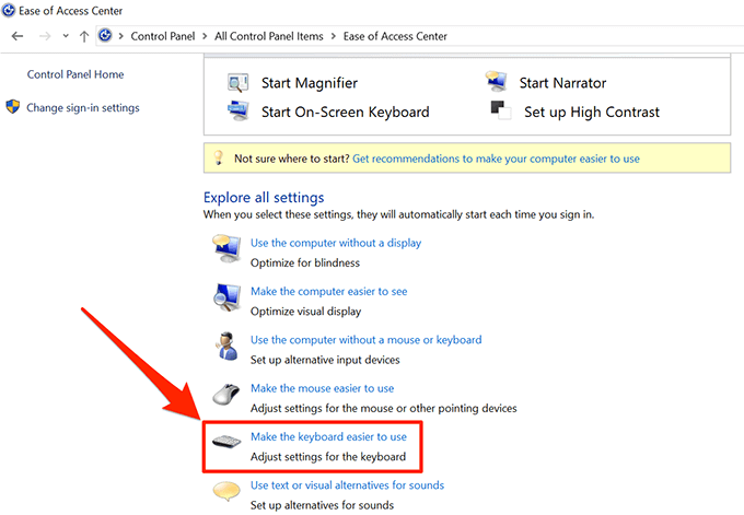
• Click on Make the keyboard easier to use.

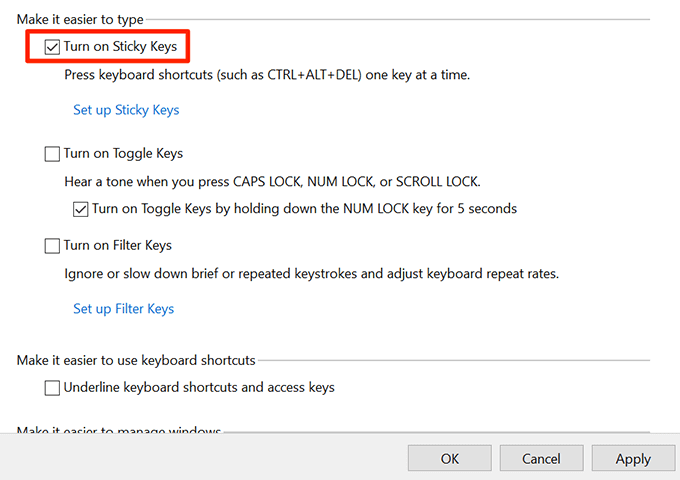
• Enable the option that says Turn on Sticky Keys and click on OK.

Disable Add-Ins

Add-ins help you get more out of Excel but sometimes they can cause conflicts as well. If you have any add-ins installed, you may want to disable them and see if the arrow keys then start working.

It’s fairly easy to disable add-ins in the Excel software.

• Launch Excel on your computer.
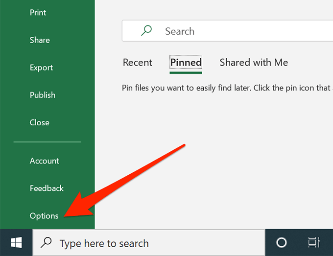
• Click on the File menu at the top and select Options from the left sidebar.

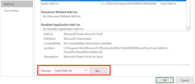
• Click on Add-ins in the left sidebar to view your Excel add-ins settings.
• Select Excel Add-ins from the dropdown menu and click on Go.

• Deselect all the add-ins and click on OK.

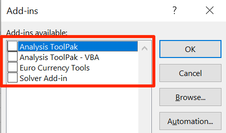
• Do the above steps for every option in the dropdown menu so that all of your add-ins are disabled.

We hope your arrow keys not working in Excel issue is now resolved. And if so, we’d like to know what method worked for you. Let us know in the comments below.

The grand job of Excel is to be an analysis tool that gives a quick visual and graphic indication of data. Arrows also play a decent role in playing up to the quick visual part.

Pointing to denote the relation between data (datasets, objects such as lists, charts, and graphs) and showing increase and decrease in numerical values are the prime reasons for using an arrow in Excel.

By the end of this tutorial, you will learn a handful of ways of inserting an arrow in Excel that are copy-pasting and using the Symbol and Shapes options, Conditional Formatting, and special fonts.

There isn’t one particular type of arrow that you’re stuck with; there’s a bunch of types you can choose from (line arrow, block arrow, pointer arrow, etc.) so why don’t we start sampling some methods?

Let’s get arrowing!

Copying & Pasting

 In the first method, we are straight up serving the option to copy the arrow from here and paste it to your work. In this form, an arrow is a text value. Let’s give you a little scenario and a small Excel trick to go with it; definitely a handy combo.

Suppose we have mapped the daily prices in dollars of an ounce of gold from 16^th June to the 1^st of July. To get an idea of the trend, we’d be eyeing a list of 6-digit numbers and what’s the point of Excel if we have to strain so much?

Here’s our objective; we’re going to add a new column to signify the trend of the gold prices with up and down arrows. Here are some arrows you might be interested in for your spreadsheet:

↑ ↓ → ← ↔ ↕

Now copy the up arrow and add it next to the increasing prices and the down arrow next to the decreasing prices. In the Excel world, that is actually a very caveman suggestion. We can make it much easier so, follow these couple of steps to insert arrows in Excel that are not so Stone Age:

• Copy the up and down arrows of choice from above and paste them separately from your dataset on the worksheet:

• Add the following formula to the trend column and copy it down so the arrows will be added for all the prices:

=IF(D4>D3,$F$3,$F$4)

This is a simple formula with the IF function that goes: if the price (in cell D4) is greater than the earlier price (in D3), then insert the up arrow (in F3) otherwise, insert the down arrow from F4. F3 and F4 have been entered as absolute references so that the references do not shift as the formula is copied down.

You can hide the off-dataset arrows in F3 and F4 by changing their font color to white. Being able to change the font color also hints that you can control the font style (including size, bold, and underline).

And that works to add the arrows in your data; no caveman in sight! Why this formula works is because the arrows in F3 and F4 are part of the cell’s value. And the IF function is asking for the result to be the value of F3 otherwise that of F4.

Being a cell value, other characters can be added to the same cell as the arrow.

You can further make this outcome more visual by adding a Conditional Formatting layer to change the up arrows to red and down arrows to green. But if we must go the Conditional Formatting way, why not just go directly? You’ll see how later.

As a text value, arrows can be added directly in the formula like so:

=IF(D4>D3,"↑","↓")

Instead of using absolute references of the cells containing the arrows, we have copy-pasted the arrows straight into the formula. You can see that the results are identical and we’ve also eliminated the need to have the arrows in F3 and F4:

Using Symbol Option

For inserting arrows in Excel (or any symbol or character for that matter), nothing will give you a more diverse line-up than Symbol. Symbol is a tool in Excel that allows the user to add a character or symbol from a grand menu to the worksheet as a cell value.

Arrows aren’t a very unusual character so you’ll find many types in Symbol using plain and symbol fonts. See the steps ahead to insert arrows in Excel with the Symbol option:

• Select the cell where you want to add the arrow.
• We will be applying the IF function as shown in the example previously so the arrows are added away from the dataset.
• In the Insert tab, select the Symbol icon from the Symbols

• This will launch the Symbol dialog box with a comprehensive spread of all types of symbols and characters imaginable:

• Using the normal text in the Font bar given at the top, enter 2190 in the Character Code
• This is the code for a leftwards arrow preceding further arrow options including diagonal and double-pointed arrows.

• Choose the arrow you want to add and then click on the Insert

• The dialog box will remain open but in the background, the chosen symbol will be added to the selected cell on the worksheet.

• Further add symbols if you wish to use more.
• Then close the Symbol dialog box with the Close

• The symbol is entered in cell edit mode.
• Click any other cell on the worksheet or press the Enter key to leave cell edit mode.
• If you have inserted multiple arrows in the cell, you can copy them in cell edit mode and paste them to other cells.

• Enter an IF formula to insert the arrows according to the cell values.

The arrows that we retrieved from Symbol will be added in the dataset:

That was what we could get using a normal font. If we change the font to a symbol or special font, we open up even more types of arrows available to us. As an example, we’ll show you what you can find using the Wingdings 3 font in Symbol since it is arrow galore:

In the fourth row, you can see some hollow arrows with shadows. Simple hollow arrows can be found with the Wingdings font. Here’s more from Wingdings 3:

Notes:

As we had done in copy-pasting, the arrows can be directly added to the formula from Symbol. While typing the formula, open the Symbol tool when you need to insert the arrow. Add the arrow, close Symbol, and continue to type the formula.

With a special font, the symbols don’t transfer well using a formula or a value paste and you will be seeing an odd character instead of the arrow. Just change the target cell’s font to the special font the arrow is from (use the Font bar on the Home tab for this) and this should return your arrow!

The reason is that inserting the arrow using a special font (let’s say Webdings font) in Symbol automatically changes the font of the cell into Webdings. But when you use a formula or paste the value of the arrow, you only get the character behind the arrow.

Changing the font to Webdings (or whichever font you have used in Symbol) will immediately fix this problem. 

Using Shapes Option

Another flexible way to add arrows is the Shapes option. Shapes offers predesigned shapes, ready to be drawn on the worksheet by clicking and dragging the mouse– far niftier than anyone’s luck at freehand. Our interest lies in the arrows we can get from Shapes so let’s have a look at what we need to do to insert arrows on the worksheet using this feature.

• Go to the Illustrations group in the Insert tab, and click on the Shapes icon to open the menu.

• Select an arrow shape of your preference from the menu.
• The Lines and Block Arrows section have all the arrows you may need. We’re adding a rightward block arrow (first arrow in Block Arrows) for our example case.

• Your mouse pointer will turn into a plus-sign cursor which is like a pen for the shape you want to insert.

• Point the cursor where you want the arrow, and click-drag the left mouse button to draw the arrow shape (it’s alright if the aim is off, you can resize, relocate and reposition the shape later).

• Adjust the style of the arrow from the Shape Format

This tab appears when the inserted shape is selected.

That’s all you need to do with the Shapes option to add an arrow!

Note: The Shapes feature would be very inconvenient to use in a dataset like our previous case example with gold rates. That is because when you insert the shape, it is inserted as an object that sits above the worksheet.

Therefore, it is not a part of a cell’s value and cannot be used as part of a formula. This means that every arrow will have to be copy-pasted. Why do that when other options can take care of automating the process? Still hung up on wanting colorful arrows like this for your data?

The next section will cover that for you.

If you need your arrows to do the talking, neighboring the Shapes option is another feature called SmartArt that will add more interactive arrows in your data and you can use this for objects like lists, processes, cycles, relationships, etc.

Using Conditional Formatting

Conditional Formatting holds the answer to so many manual Excel woes. This feature uses colors, icons, or bars to change the display of cells according to their value. You see where we’re going with this? How about we try to get Conditional Formatting to display arrows, the colorful kind, according to the numeric value in the cell? Check out the steps ahead where we apply Conditional Formatting to insert arrows in Excel:

We’re going to switch up our case example a bit. Let’s carry forward the example involving gold rates and assume a seller’s point of view. So that when gold rates would drop, that is negative for the seller and the increase is positive. The steps begin:

• In the column where you want to display the arrows, enter a formula calculating the difference of the prices with the preceding day e.g. =D4-D3 gives us the difference between the prices of the 16^th and 17^th of June.
• Fill the column with this formula.

• Select the cells with the formula (these are the values that the arrows will replace).
• Open the Conditional Formatting menu from the Home tab’s Styles Point to Icon Sets in the menu and select More Rules.

• Make these changes in the New Formatting Rule dialog box:
• Choose the arrow style from the Icon Style drop-down menu.
• Check the Show Icon Only checkbox (this replaces the cell value and displays the icons otherwise the icons appear with the values).
• In the Type section, change all three fields to Number instead of Percent.
• Change the first value from the Value section to 1 instead of 0.

• Hit the OK button when done.

The arrow icons have been applied to the data. Where the price is lesser than the previous price, Conditional Formatting has displayed a red arrow and for an increase, it displays a green arrow.

Note: Conditional Formatting does not allow relative references in Icon Sets, Data Bars, and Color Scales so you won’t be able to have the arrows displayed in column D in this scenario. However, if the arrows were to be added against a fixed number or an absolute reference, they could be displayed in the same cells as the values.

Using Custom Format

This is another pretty cool Excel trick and we’ll show you how to make it even cooler. Not only can you use a custom number format to display arrows in cells, but you can also have the positive figures appear green and the negative figures appear red. Fancy! If that’s a tad too fancy for you, we’ll also show you how to display arrows in a cell without changing the font color.

Do take note that this will not add an arrow in a cell and therefore it won’t alter the cell’s value; this is a format and will only display the arrow, keeping the value intact so the numbers can be used further in number formulas. Now would be a good time to demonstrate how to do that. Follow the steps ahead to display arrows using Custom Format.

In this case example, we have a simple monthly sales report for the years 2025 and 2026 with the variance per month calculated.

We aim to display arrows in the variance column so, go through the steps below to do the same for your work:

• Select the target cells for the arrows. We’ve selected the cells with the variances i.e. F4:F15.
• Click on the Number group’s dialog box launcher.

• The Format Cells dialog box will be launched with the Number tab open. And if you head to the Custom category on the left, you will see the current format of the selected cells:

• This is the format we want to change.
• In the Type box, replace the current format with this custom formatting code:
• For displaying arrows without changing the font color:

↑ $0;↓ -$0

We have copy-pasted the arrows in this formatting code. As per the code, a positive number will be displayed with an upwards arrow and a negative one with a downwards arrow. Applied to the selected cells, this is how it turns out:

But we were talking about some color splash, remember? Use this formatting code instead if you want green and red arrows:

• For displaying green and red arrows for positive and negative values respectively:

[Green] ↑ $0;[Red] ↓ -$0

This formatting code displays the arrows as well as formats the font color of positive values as green and negative values as red. The Sample field will give you a preview of the format when it recognizes the formatting code.

• Select the OK button to apply the format to the selected cells.

Arrows and font colors aptly formatted:

Neat!

Note: The font color set in the formatting code cannot be changed from the active worksheet.

Using Special Fonts

And lastly, arrows can be added in Excel using special fonts. If that sounds familiar, 10 points to you because you’re right; we discussed using special fonts via the Symbol feature. Now we’ll talk about using special fonts directly on the active worksheet.

How is this going to work? You need to enter (type, paste, or insert) a character and change the font of that cell to a special font so that it returns an arrow. Which font and what character? Every special font turns a character into a different symbol. E.g. an exclamation point «!» will be a spider web symbol with the Webdings font, pencil with Wingdings, pen with Wingdings 2, and a left arrow with the Wingdings 3 font.

Taking cue from there, we’ll show what characters you need for different arrows. There are many more types of arrows that can be accessed with special fonts and you are free to explore them but our suggestion below includes easy characters that you can type from your keyboard. Here’s what you need to do.

• Add the character to the cell where you want the arrow.
• The characters and their corresponding arrows with the Wingdings 3 font are mentioned below:

Font: Wingdings 3

We’re entering a number sign «#» in cell F4 and a dollar sign «$» in F5 to get the up and down arrows.

Select these cells and change the font to Wingdings 3. This won’t change the font of the results of the function but this way you can confirm if you’re putting the right character through.

• Enter the formula in the cells where you want the arrows.
• You should be seeing the characters (number and dollar sign in our case example) as the formula’s results.

• Select the characters and change the font to the respective special font (Wingdings 3 for us).

You should successfully have the arrows in place!

The Formula Bar displays the character when you select the original arrow and the special font can be viewed in the Font bar. As a cell value, the arrow can remain in the special font while other characters and values can be added in the same cell in regular fonts:

The pro? You won’t have to access any other feature for the arrows. The con? You still need to know which character will return what arrow.

That’s all there’s up with inserting arrows in Excel. All the methods add arrows to the cell value except for the Shapes option which inserts the arrow above the worksheet and the Custom Format which only displays arrows. Arrows (as text values) can be used as part of formulas and formatting codes. We hope we’ve «pointed» you in the right direction.