
Excel for Microsoft 365 Excel for Microsoft 365 for Mac Excel for the web Excel 2021 Excel 2021 for Mac Excel for iPad Excel for iPhone Excel for Android tablets Excel for Android phones More…Less
#CALC! errors occur when Excel’s calculation engine encounters a scenario it does not currently support. Here’s how to address specific #CALC! errors:
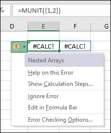
Excel can’t calculate an array within an array. The nested array error occurs when you try to input an array formula that contains an array. To resolve the error, try removing the second array.
For example, =MUNIT({1,2}) is asking Excel to return a 1×1 array, and a 2×2 array, which isn’t currently supported. =MUNIT(2) would calculate as expected.
Arrays can only contain numbers, strings, errors, Booleans, or linked data types. Range references aren’t supported. In this example, =OFFSET(A1,0,0,{2,3}) will cause an error.
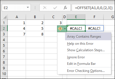
To resolve the error, remove the range reference. In this case, =OFFSET(A1,0,0,2,3) would calculate correctly.
Excel can’t return an empty set. Empty array errors occur when an array formula returns an empty set. For example, =FILTER(C3:D5,D3:D5<100) will return an error because there are no values less than 100 in our data set.
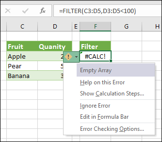
To resolve the error, either change the criterion, or add the if_empty argument to the FILTER function. In this case, =FILTER(C3:D5,D3:D5<100,0) would return a 0 if there are no items in the array.
Custom functions that refer to more than 10,000 cells cannot be calculated in Excel for the web, and will produce this #CALC! error instead. To fix, open the file in a desktop version of Excel. For more information, see Create custom functions in Excel.
This function performs an asynchronous operation but has unexpectedly failed. Try again later.
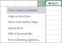
A LAMBDA function behaves a little differently than other Excel functions. You can’t just enter it into a cell. You must call the function by adding parentheses to the end of your formula and passing the values to your lambda function. For example:
-
Returns the #CALC error:
=LAMBDA(x, x+1) -
Returns a result of 2:
=LAMBDA(x, x+1)(1)
For more information, see LAMBDA function.
This error occurs when Excel’s calculation engine encounters an unspecified calculation error with an array. To resolve it, try rewriting your formula. If you have a nested formula, you can try using the Evaluate Formula tool to identify where the #CALC! error is occurring in your formula.
Need more help?
You can always ask an expert in the Excel Tech Community or get support in the Answers community.
See Also
Dynamic arrays and spilled array behavior
Need more help?
Want more options?
Explore subscription benefits, browse training courses, learn how to secure your device, and more.
Communities help you ask and answer questions, give feedback, and hear from experts with rich knowledge.
Does your Excel showing you cannot change part of an array error? But you don’t have any idea why you are getting this error and how to fix this?
Well, in that case, this blog is really gonna help you a lot. As it covers detailed information on Excel error you cannot change part of an array and ways to resolve this.
What Does You Can’t Change Part Of An Array Mean?
Excel array formula is one such formula that can execute multiple calculations over single or multiple numbers of items in the array.
You can consider this array as the combination of value’s rows and columns. Array formula can give you single or multiple results in return.
Suppose, in the range of cells you can also make the array formulas and can use the array formula for calculating column or row. Just place the array formula within a single cell for making the calculation of a single amount.
Array formula which is having multiple cells is known as a multi-cell formula. Whereas, the array formula present in the single-cell is known as the single-cell formula.
This Excel error you can’t change part of an array arises due to the issue in the range of array formula. Now you need to choose entire cells from that array before making any changes to it.
Here is the screenshot of this error:

Method 1# Match The Syntax
Usually, the array formulas strictly follow the standard formula syntax. It starts with an equal sign.
In the array formulas, you can use the Excel built-in functions. So, make a press over the Ctrl+Shift+Enter for entering the formula.
Excel closes array formula within the braces. But if you manually add these braces then the array formula will get converted to the text string and this won’t work correctly.
To build a complex formula, Array functions are quite an efficient option to choose from.
Suppose you are using complex formula like this: =SUM(C2*D2,C3*D3,C4*D4,C5*D5,C6*D6,C7*D7,C8*D8,C9*D9,C10*D10,C11*D11).
So instead of using the above complex formula, you can use the array formula =SUM(C2:C11*D2:D11)
To extract data from corrupt Excel file, we recommend this tool:
This software will prevent Excel workbook data such as BI data, financial reports & other analytical information from corruption and data loss. With this software you can rebuild corrupt Excel files and restore every single visual representation & dataset to its original, intact state in 3 easy steps:
- Download Excel File Repair Tool rated Excellent by Softpedia, Softonic & CNET.
- Select the corrupt Excel file (XLS, XLSX) & click Repair to initiate the repair process.
- Preview the repaired files and click Save File to save the files at desired location.
Method 2# Rules For Changing Array Formulas
If you are rigorously trying to make changes in the formula bar or in the formula cell. But every time you are getting the same you cannot change part of an array error.
In that case, quickly make a cross-check over the below-mentioned array formula guidelines.
Breaking the rules for changing array formulas also results in you cannot change part of an array error.
- If you are entering a single-cell array formula, then choose the cell and hit the F2 button to make easy changes.
- After that press the Ctrl+Shift+Enter button from your keyboard.
- If in case, you are entering the multi-cell array formula then choose the entire cell having this formula and then press the F2 button. after that below mentioned set of rules:
- You are not allowed to move individual cells having the formula, but as a group, you can all of them at once. Ding this will automatically change the formula cell references accordingly.
To shift this to a new place, choose the entire cell and press the Ctrl+X. Choose any new location, where you want to paste it. After that make a press over the Ctrl+V button.
- In the array formula, you can’t delete any cells if you are trying to do so then it’s obvious to get the “You cannot change part of an array”
But you have the option to delete the complete formula and then start again from the beginning.
- Nor, you can’t add new cells to the section of result cells. But you have the option to add new data within your Excel worksheet and then expand the array formulas.
- After doing complete changes, hit the Ctrl+Shift+Enter.
Using the array constants (part of array formula which is typed in formula bar) you can easily save up your time. But remember one thing that array constants also have a few usage and editing rules.
Method 3# Use Ctrl+Shift+Enter
It is the basic and most important component of array formulas which you need to enter by using the Ctrl+Shift+Enter.
Here are the steps to create an array formula:
- Choose cells that contain the array formula.
- Assign the formula either by typing or using the formula bar.
- After completing all these, enter the formula and then type Ctrl+Shift+Enter.
- Just put the formula within the array.
Method 4# Use Names To Refer To Arrays
One plus point about the Excel arrays is that it offers the option of including the named ranges. One can use these named ranges either in the time-series or to the table formulas which is enforced for using the cell references.
With the array formulas, you will see that your spreadsheet formula will be easier to read and interpret with named cells.
Method 5# Select Arrays With A Keyboard Shortcut
If you are working with an already existing cell array formula then it’s important to choose and edit the complete array.
It’s quite tedious but there are some shortcuts available to use this.
- To select the cell of array press the “Ctrl” and forward-slash (“/”). Similarly, you can select the entire array.
- Press the F2 key or you can edit the formula present within the formula bar.
Last but not least after completing all this just type Ctrl+Shift+Enter.
Method 6# Remove Part Of An Array In Excel
If the above fixes won’t resolve the error you cannot change part of an array then try removing some part of your array. Doing this will definitely going to work.
After deleting up the formula, you will see that result of the formula is also gets deleted. If you don’t want to remove the values then only remove the formula.
Learn how both these tasks should be performed.
Delete A Formula But Keep The Results
For deleting up the formula and keeping up the result you need to copy the formula after that paste it in the same cell. But this time you have to use the Paste Values option.
1. Choose the cell ranges or cells having the formulas in them. If you have used the array formula, then firstly you need to choose the cells present in the ranges of the cells having the array formula.
- Tap to the cell in the array formula.
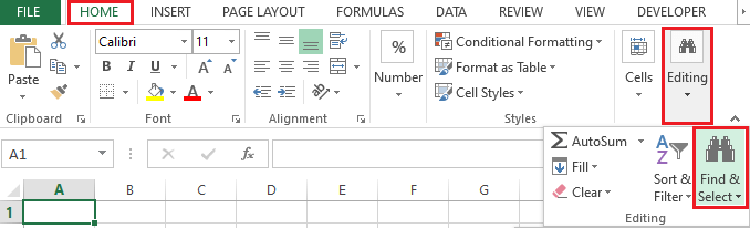
- Hit the Home tab, and then from the Editing group, choose the Find & Select.
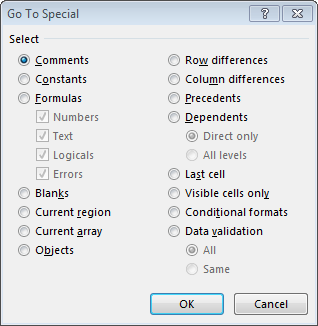
- After that tap to the Go To > Special > Current array.
2. Go to the Home tab and then from the Clipboard group, choose the Copy

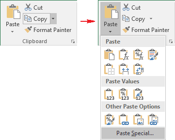
3. Go to the Home tab and then from the Clipboard group, tap the arrow present below the Paste button, and then hit the Paste Values.
Delete An Array Formula
For deleting up the array formula, choose all cells to present within the range of cells having the array formula in it. After that perform the following step:
- Tap to the cell present in the array formula.
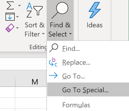
- Go to the Home tab, in the Editing group, click Find & Select, and then click Go To.
- Click Special>Current array
- At last hit the DELETE
Wrap Up:
Undoubtedly, using the Array formulas is a great option to use but it has disadvantages too. I have noticed the following points.
As per the processing speed and computer memory, large array formulas may result in slower calculation.
Other Excel workbook users maybe won’t understand the formula. Generally, array formulas are not explained within the worksheet.
So if any other user needs to edit the workbooks then it’s compulsory for them to have knowledge about array formulas or you need to avoid the array formulas.


Priyanka is an entrepreneur & content marketing expert. She writes tech blogs and has expertise in MS Office, Excel, and other tech subjects. Her distinctive art of presenting tech information in the easy-to-understand language is very impressive. When not writing, she loves unplanned travels.
Microsoft Excel is a spreadsheet program developed and distributed by Microsoft. It is available across almost all platforms and is used extensively for business and other purposes. Due to it’s easy to use interface and numerous formulas/functions, it has made easy documentation of data a reality. However, quite recently, a lot of reports have been coming in where users are unable to apply a formula to replace a specific letter for a word and an “An Array Value Could not be Found” Error is displayed.
Usually, there are many formulas that can be applied to make entrail certain commands. But users experiencing this error are unable to do so. Therefore, in this article, we will be looking into some reasons due to which this error is triggered and also provide viable methods to fix it.
What Causes the “An Array Value Could not be Found” Error on Excel?
After receiving numerous reports from multiple users, we decided to investigate the issue and looked into the reasons due to which it was being triggered. We found the root cause of the issue and listed it below.
- Wrong Formula: This error is caused when the substitution formula is entered incorrectly. Most people use the substitution formula to replace a specific letter with a word or a line. This ends up saving a lot of time but if entered incorrectly this error is returned.
Now that you have a basic understanding of the nature of the problem, we will move on towards the solutions. Make sure to implement these in the specific order in which they are presented to avoid conflict.
Solution 1: Using Substitute Array Formula
If the formula has been entered incorrectly, the substitution function will not work properly. Therefore, in this step, we will be using a different formula to initiate the function. For that:
- Open Excel and launch your spreadsheet to which the formula is to be applied.
- Click on the cell to which you want to apply the formula.

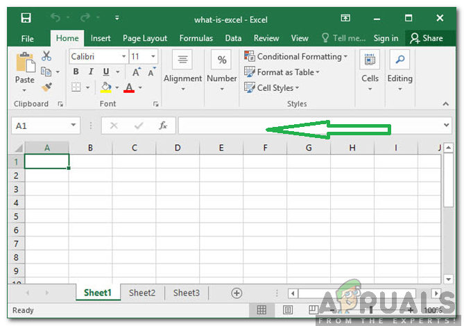
Selecting the cell - Click on the “Formula” bar.
- Type in the following formula and press “Enter”
=ArrayFormula(substitute(substitute(substitute(E2:E5&" "," y "," Y ")," yes "," Y ")," Yes "," Y "))
- In this case, “Y” is being replaced with “Yes“.
- You can edit the formula to fit your needs, place the letter/word that needs to be replaced in place of “Y” and the letter/word that it needs to be replaced with needs to be placed in the place of “yes”. You can also change the address of cells accordingly.
Solution 2: Using the RegExMatch Formula
If the above method didn’t work for you, it is possible that by approaching the problem with a different perspective might solve it. Therefore, in this step, we will be implementing a different formula which uses a different set of commands to get the work done. In order to apply it:
- Open Excel and launch your spreadsheet to which the formula is to be applied.
- Click on the cell to which you want to apply the formula.
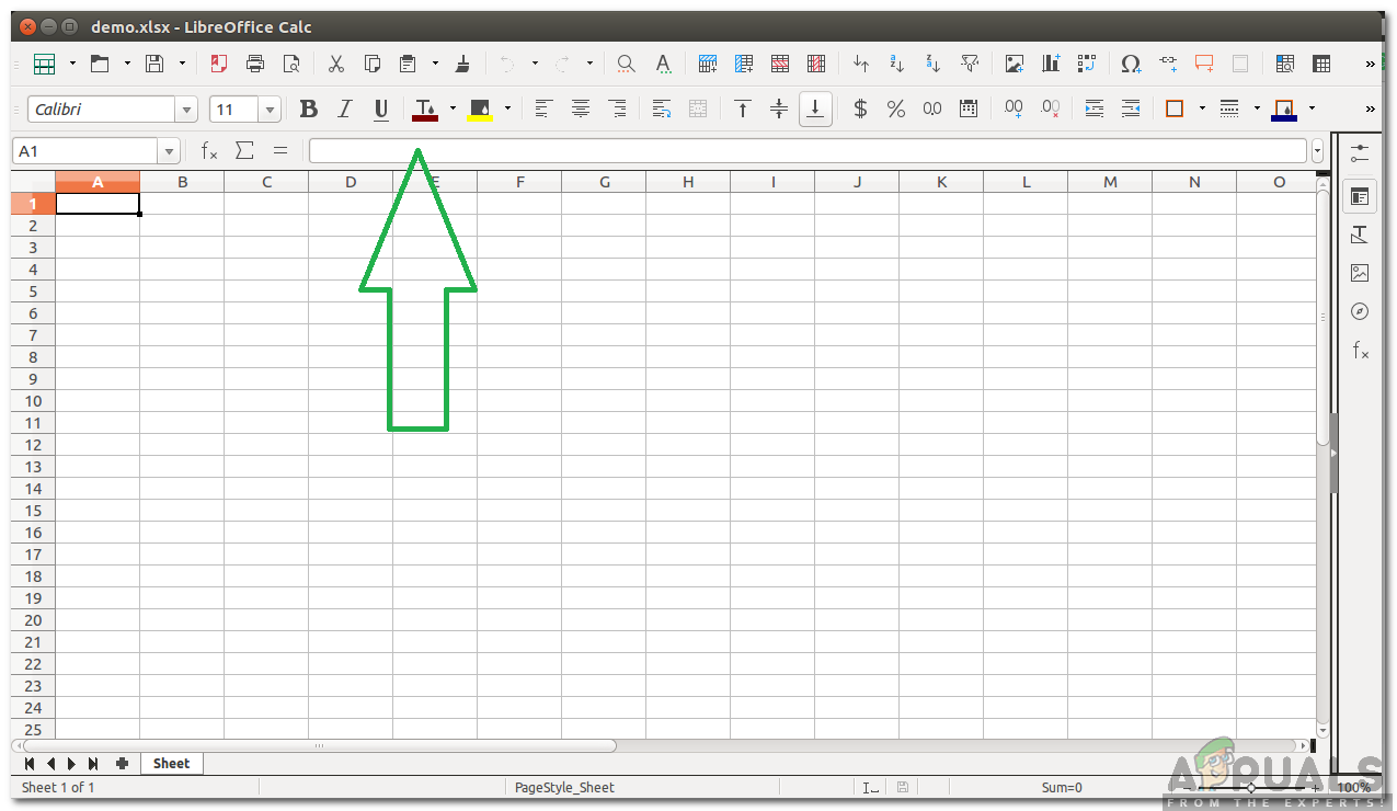
- Select the “Formula” bar.

Selecting the formula bar - Enter the formula written below and press “Enter”
=if(REGEXMATCH(E2,"^Yes|yes|Y|y")=true,"Yes") - This also replaced “Y” with “Yes”.
- The values for “Y” and “Yes” can be changed to fit your needs.
Solution 3: Using Combined Formula
In some cases, the combined formula generated from the above mentioned two formulas gets the trick done. Therefore, in this step, we will be using a combined formula to fix the error. In order to do that:
- Open Excel and launch your spreadsheet to which the formula is to be applied.
- Select the cell to which you want to apply the formula.
- Click on the “Formula” bar.

Clicking on the formula bar - Enter the formula mentioned below and press “Enter”
=ArrayFormula(if(REGEXMATCH(E2:E50,"^Yes|yes|Y|y")=true,"Yes")) - This replaces “Y” with “Yes” as well and can be configured to fit your conditions accordingly.
Solution 4: Using RegExReplace Formula
It is possible that the “RegExReplace” formula might be required to eradicate the error. Therefore, in this step, we will be using the “RegExReplace” formula in order to get rid of the error. For that:
- Open Excel and launch your spreadsheet to which the formula is to be applied.
- Select the cell to which you want to apply the formula.
- Click on the “Formula” bar.

Clicking on the Formula bar - Enter the formula mentioned below and press “Enter”
=ArrayFormula(regexreplace(" "&E2:E50&" "," y | yes | Yes "," Y ")) - This replaces “Y” with “Yes” and can be configured to fit your situation accordingly.

Kevin Arrows
Kevin Arrows is a highly experienced and knowledgeable technology specialist with over a decade of industry experience. He holds a Microsoft Certified Technology Specialist (MCTS) certification and has a deep passion for staying up-to-date on the latest tech developments. Kevin has written extensively on a wide range of tech-related topics, showcasing his expertise and knowledge in areas such as software development, cybersecurity, and cloud computing. His contributions to the tech field have been widely recognized and respected by his peers, and he is highly regarded for his ability to explain complex technical concepts in a clear and concise manner.
Using Microsoft Excel allows us to organize our data more efficiently. With Google Sheets, you can immediately save the file on the cloud and access it at any time on any device.
However, some users encounter the “An Array Value Could not be Found” error message when they try to edit the cells on a Microsoft Excel or Google Sheets spreadsheet. If you experience the same issue, there are several ways on how you can fix it.
How to Fix ‘An Array Value Could Not Be Found’ Error in Microsoft Excel or Google Sheets
An array consists of several rows and columns with values. You can group your cells using arrays. To solve the issue with the array value on Windows 10 or Mac computer or any browser, you can use any of the formulas stated below.
Method#1 – Add the ARRAYFORMULA Word to Your Substitute Formula
To do this method, you will need to add ARRAYFORMULA at the beginning of your Substitute Formula.
- On your Microsoft Excel or Google Sheets, look for the cell with the substitute formula.
- Click on it and go to the Formula bar.
- After the Equal Sign, add the word, ARRAYFORMULA. For instance, =ARRAYFORMULA(SUBSTITUTE(A1:A2, “N”, “No”))
Method #2 – Use the REGEXMATCH Formula
Another method you can use on your Microsoft Office Excel or Google Sheets is the REGEXMATCH formula.
- Look for the cell that you want to edit and highlight it.
- Go to the Formula bar.
- Enter the following: =if(REGEXMATCH(E2,”^Yes|yes|Y|y”)=true,”Yes”)
Method #3 – Make Use of REGEXREPLACE
If you don’t want to use REGEXMATCH, you can also use REGEXREPLACE. The method is the same.
- First, highlight the cell that you want to change.
- On the Formula bar, type the following: =ArrayFormula(regexreplace(” “&B2:B4&” “,” Yes | Y | Y “,” Yes”))
Method #4 – Combine ARRAYFORMULA and REGEXMATCH
There is another formula that uses both ARRAYFORMULA and REGEXMATCH.
- Click the cell that you want to edit.
- On the Formula bar, enter the following: =ArrayFormula(if(REGEXMATCH(E2:E50,”^Yes|yes|Y|y”)=true,”Yes”))
Note that you can always edit the formula based on your preferences.
Which of the methods above work for you best? You can let us know by writing us a comment down below.
#CALC! error appears when an array-related calculation error is encountered in Excel. Array formulas allow you to work with several values in one formula and let you perform different calculations simultaneously.
The #CALC! error is mainly associated with dynamic arrays introduced in Excel Office 365; therefore, you will not face this error in older versions of Excel. You might also face this error whilst using the FILTER and LAMBDA functions.
To resolve this, try rewriting your formula or look at some examples below for a better understanding.

What is a #CALC! Error in Excel?
The #CALC! error mainly arises when the calculation engine of Excel faces an unexpected issue with the dynamic array formulas.
The best way to solve the #CALC! error in Excel is by going back to the basics and rewriting the formula, referring to the syntax of the functions used.
If your formula is nested, you can try utilizing the Evaluate Formula tool (from the Formulas tab > Formula Auditing group > Evaluate Formula) to find the location of the #CALC! error.
Scenarios in which #CALC! Error can Occur
Below are some scenarios of when you could face the #CALC! error along with examples and solutions.
Scenario 1: Empty Array in FILTER Function
If the formula entered returns an empty array, you would get a #CALC! error. When using the FILTER function, #CALC! error is encountered when the query results have no matching data. In such a case, since Excel can’t return an empty array so it returns a #CALC! error.
Let’s try to understand this with an example.
Example 1
In this case, we are looking at the cumulative grade point average of a class of engineering students. Using the FILTER function, we will try to obtain the details of the students with a CGPA of less than 4. The formula below seems like a good place to start with:
=FILTER(A2:C13,C2:C13<4)
We have mentioned the range containing the data i.e. A2:C13 in the first parameter followed by the condition C2:C13<4 that the values in column C are to be checked for values less than 4.

As you can see, there are no candidates with less than a 4 CGPA, and the result is empty. Therefore, Excel returns a #CALC! error. This is because we’ve missed out on the if_empty argument. This is the 3rd argument of the function. Here you need to specify what value the function should return in case it results in an empty array.
Resolution
When using the FILTER function, #CALC! error occurs when the query results in an empty array. Therefore, you must mention the if_empty condition.
To get rid of the error, we’ve taken the formula below into action:
=FILTER(A2:C13,C2:C13<4,"NULL")
In the given example, adding «NULL» or anything you wish to display if there is no matching result. This means that if there is no one with less than 4 CGPA, return the value NULL. Enclose the value (as we have done with NULL) in double-quotes. If you don’t want any value displayed for an empty array, you can add «» which is an empty text string.

Another way to resolve the #CALC error is by adjusting the logic in the function’s first argument, so no empty value is returned.
Example 2
The data set we are using in this example contains the date and location of a list of events. For the purpose of planning, it would be helpful to know what events will take place between two dates. Now let’s see if there are any events between 1st Dec 2022 & 31 Dec 2022.
Using the FILTER function, we have come up with this formula:
=FILTER(A2:C10,(A2:A10>=F1)*(A2:A10<=F2))

The #CALC! error occurs as there are no events between those two dates.
Resolution
To resolve the #CALC! error, we can add a condition that if there are no events that fall in the mentioned criteria, display «No Events». This condition will be added in double-quotes as the if_empty argument. The formula is amended as follows:
=FILTER(A2:C10,(A2:A10>=F1)*(A2:A10<=F2),"No Events")

Scenario 2: Excel Web
As per the official website, when using Excel Web, you might face a #CALC! error if your calculation involves more than 10,000 cells. In Excel for the web, custom functions with references to more than 10,000 cells cannot be computed and instead result in the #CALC! error.
Scenario 3: While using LAMBDA Function
LAMBDA function allows you to create a custom Excel function. Once a LAMBDA function is created and saved, it can be inserted multiple times in a workbook.
As the LAMBDA function provides a way to create a custom function in Excel, you can develop a function for a frequently used formula and avoid copying and pasting it.
But it is important to note that it cannot be used directly without a cell reference. You will see a #CALC! error because the function needs a reference from where data can be used.
It is further explained with an example.
Example 1
You wish to convert the GBP into USD.
In general use, you would use GBP/Conversion Rate if you’re punching figures on your calculator. In Excel, if you have multiple values to convert, you would give reference to the cell containing the GBP value as done in the formula ahead:
=A2/0.83

If you wish to use the LAMBDA function to carry out this conversion, you will have the advantage of being able to use the created formula throughout the workbook. To achieve that, let’s give this formula a go:
=LAMBDA(x,x/0.83)
This will give you a #CALC! error as there are no references to any cells for «x». The formula has no input values to calculate with, hence it returns the #CALC! error.

Resolution
Excel gives a #CALC! error if you assemble a LAMBDA function in a cell without giving it any references to work with. You must add parentheses with the relevant cell reference(s) to the end of your formula to call the function and provide the values to your LAMBDA function.
Let’s fix the previously used formula, supplying the necessary cell reference, and see if it resolves the error for us:
=LAMBDA(x,x/0.83)(A2)

Providing the LAMBA function with A2 as the cell reference, we have successfully fixed the error! Win-win!
Example 2
Let’s try using two parameters in the LAMBDA function. This is another point where the #CALC! error might occur.
Our example consists of two columns; one with the values of x, and the other with values of y. If we are to calculate the value of x2+ y2, we will sum the square of x value with the square of y value. If we put this together using the LAMBDA function, we can make our own formula:
=LAMBDA(X,Y,X^2+Y^2)
We are using the LAMBDA function to sum x raised to power 2 by y raised to power 2.

This will result in an error as you can see Excel will not understand what x and y are.
Resolution
We must give the cell reference to feed the value of x and y and resolve the error. Adding the cell references to our example formula gives us:
=LAMBDA(X,Y,X^2+Y^2)(A2,B2)
Adding the values from the first row in the dataset resolves the #CALC errors for us and performs the required calculation:

With all the above examples, hopefully, you have understood the possible scenarios where you might face the #CALC! error and how to resolve it. While you practice resolving #CALC! errors, we’ll have some more tutorials ready for you.
by Matthew Adams
Matthew is a freelancer who has produced a variety of articles on various topics related to technology. His main focus is the Windows OS and all the things… read more
Updated on March 4, 2021
- Google Sheets is a great web alternative for those that don’t have Microsoft Excel.
- This guide will show you how to fix the array value could not be found error in Sheets.
- If you need more tutorials about this program, check out our Google Sheets Hub.
- For more articles about this amazing software suite, check out our Googles Docs page.

XINSTALL BY CLICKING THE DOWNLOAD FILE
This software will keep your drivers up and running, thus keeping you safe from common computer errors and hardware failure. Check all your drivers now in 3 easy steps:
- Download DriverFix (verified download file).
- Click Start Scan to find all problematic drivers.
- Click Update Drivers to get new versions and avoid system malfunctionings.
- DriverFix has been downloaded by 0 readers this month.
Google Sheets is among the best freely available spreadsheet app alternatives to Excel. Sheets includes a SUBSTITUTE formula that enables you to replace a specific letter (or text string) in one cell with a word.
The cell that includes the SUBSTITUTE formula can display the replaced text for one cell.
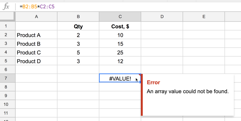
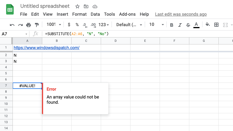
However, the SUBSTITUTE formula can’t display replaced text output for a range of cells. If you include a cell range within it, the formula’s cell will display an Array value could not be found error message as shown in the snapshot directly below.
If you’re wondering how to fix that error so that SUBSTITUTE can be applied to a range of cells, check out the resolutions below.

How can I fix the array value error for SUBSTITUTE?
1. Turn the SUBSTITUTE formula into an array formula
To fix the Array value could not be found error, you need to incorporate SUBSTITUTE within an array formula. An array formula is one that can return multiple output for a range of cells.
Thus, users who need to replace text in range of cells and then display the output in another range need to utilize an array formula.
So, what you need to do is add ARRAYFORMULA to the beginning of the SUBSTITUTE formula. To do that, select the cell that includes the SUBSTITUTE formula.
Then click in the formula bar, enter ARRAYFORMULA just after the equals (=) sign as shown in the snapshot directly below.

Then your SUBSTITUTE formula will display replaced text output for a range of cells instead of an array error.
In the example shown in the snapshot directly below, the formula replaces Y in three column cells with Yes and displays the output across three other cells below them.

2. Enter the REGEXMATCH formula instead
Alternatively, you could combine REGEXMATCH with an array formula for the same output.
- To do that, open the Sheet spreadsheet you need to add the formula to.
- Select a cell to include the formula in (it will display output across multiple cells).
- Then copy this formula with the Ctrl + C hotkey: =ArrayFormula(if(REGEXMATCH(B2:B4,”^Yes|yes|Y|y”)=true,”Yes”)).
- Click inside Sheets’ formula bar.
- Paste the REGEXMATCH formula into Sheet’s formula bar by pressing Ctrl + V.

- That formula replaces Y with Yes for the cell range B2:B4.
- You’ll need the change the Y and Yes text in the formula to whatever you need for it.
- In addition, you’ll need to change the cell reference in that formula to match your own requirements.

3. Enter the REGEXREPLACE formula
- REGEXREPLACE is another alternative you can try when your SUBSTITUTION formula doesn’t return the expected output.
- Open Sheets in a browser.
- Select a cell for the REGEXREPLACE formula.
- Copy this formula: =ArrayFormula(regexreplace(” “&B2:B4&” “,” Yes | Y | Y “,” Yes”)).
- Click within the formula bar, and press the Ctrl + V hotkey to paste the formula.

- Thereafter, edit the REGEXREPLACE formula’s referenced Y and Yes text to whatever text you need to substitute.
- Change that formula’s cell reference to meet the requirements of your spreadsheet.

So, that’s how you can fix the Array value could not be found error in Google Sheets. The overall resolution is to combine SUBSTITUTE, REGEXREPLACE, or REGEXMATCH with array formulas so that they display replaced (or substituted) text output across a range of cells.
Let us know if you found this tutorial to be useful by leaving us a message in the comments section below.
Still having issues? Fix them with this tool:
SPONSORED
If the advices above haven’t solved your issue, your PC may experience deeper Windows problems. We recommend downloading this PC Repair tool (rated Great on TrustPilot.com) to easily address them. After installation, simply click the Start Scan button and then press on Repair All.
![]()
Newsletter
Explanation
With the introduction of Dynamic Arrays in Excel formulas, there is more emphasis on arrays. The #CALC! error occurs when a formula runs into a calculation error with an array. The #CALC! error is a «new» error in Excel, introduced with dynamic arrays. It will not appear in older versions of Excel.
Empty array
An empty array can trigger a #CALC! error, and this is the most common reason you may see a #CALC! error in a worksheet, especially when using the FILTER function. This is because FILTER returns a #CALC! error when no values meet criteria – in other words, FILTER returns an empty array.
For example, in the screen below, the FILTER function is set up to filter the source data in B5:D11. However, the formula is asking for all data in the group «x», which doesn’t exist. The result is a #CALC! error:

=FILTER(B5:D11,B5:B11="x") // no such group, empty array
Fix #1 — adjust filter logic
One option to fix this error is to adjust the filter criteria to return valid results. In the screen below, the formula has adjusted to filter on group «A», and the formula works normally:

=FILTER(B5:D11,B5:B11="a") // group "a" exists; no empty array
Fix #2 — set is_empty argument
Another option is to provide a «not found» value to return when no results are returned. In the screen below FILTER returns «No results» instead of an error:

=FILTER(B5:D11,B5:B11="x","No results") // message instead of error
Note: Microsoft documentation mentions other cases that may cause #CALC! errors, notably nested arrays, and unsupported arrays. However, I have not been able to reproduce the error with the examples provided. If you have examples of formulas that throw #CALC! errors, please let me know.
Updated April 2023: Stop getting error messages and slow down your system with our optimization tool. Get it now at this link
- Download and install the repair tool here.
- Let it scan your computer.
- The tool will then repair your computer.
Table formulas in Excel are an extremely powerful tool and one of the most difficult to master. A single Excel table formula can perform several calculations and replace thousands of common formulas. Yet 90% of Excel users have never used the table functions in their worksheets simply because they are afraid to learn them.

Essentially, a table in Excel is a collection of elements. The elements can be text or numbers and can be in a single row or column or in several rows and columns. A table formula is a formula that can perform several calculations for one or more elements of a table. You can consider a table as a row or column of values, or a combination of rows and columns of values. Table formulas can return either multiple results or a single result.
Use of alternative table formulas
If the formula was entered incorrectly, the substitution function does not work correctly. Therefore, in this step, we will use a different formula to start the function. For that:
- Open Excel and start the spreadsheet to which you want to apply the formula.
- Click on the cell to which you want to apply the formula.
- Click on the formula bar.
- Enter the following formula and press Enter.
=ArrayFormula(substitute(substitute(substitute(E2:E5&” “,” y “,” Y “),” yes “,” Y “),” Yes “,” Y “))
In this case, “O” is replaced by “Yes”.
April 2023 Update:
You can now prevent PC problems by using this tool, such as protecting you against file loss and malware. Additionally it is a great way to optimize your computer for maximum performance.
The program fixes common errors that might occur on Windows systems with ease — no need for hours of troubleshooting when you have the perfect solution at your fingertips:
- Step 1 : Download PC Repair & Optimizer Tool (Windows 10, 8, 7, XP, Vista – Microsoft Gold Certified).
- Step 2 : Click “Start Scan” to find Windows registry issues that could be causing PC problems.
- Step 3 : Click “Repair All” to fix all issues.

You can customize the formula according to your needs, replace “Y” with the letter or word you want to replace and “yes” with the letter or word you want to replace. You can also change the address of the cells accordingly.
Using the RegExMatch formula
If the above method has not worked for you, it is possible that by approaching the problem from a different perspective it can be solved. Therefore, in this step, we will implement a different formula that uses a different set of commands to do the work. To apply it:
- Open Excel and start the spreadsheet to which you want to apply the formula.
- Click on the cell to which you want to apply the formula.
- Select the formula bar.
- Enter the formula below and press Enter.
=if(REGEXMATCH(E2,”^Yes|yes|Y|y”)=true,”Yes”)
He also replaced “O” with “Yes”.
The values for “Y” and “Yes” can be adapted to your needs.
https://stackoverflow.com/questions/47569464/array-value-not-found-error
Expert Tip: This repair tool scans the repositories and replaces corrupt or missing files if none of these methods have worked. It works well in most cases where the problem is due to system corruption. This tool will also optimize your system to maximize performance. It can be downloaded by Clicking Here

CCNA, Web Developer, PC Troubleshooter
I am a computer enthusiast and a practicing IT Professional. I have years of experience behind me in computer programming, hardware troubleshooting and repair. I specialise in Web Development and Database Design. I also have a CCNA certification for Network Design and Troubleshooting.
Post Views: 414
Can anyone help me?
I have been getting a compile error (…: «Expected Array») when dealing with arrays in my Excel workbook.
Basically, I have one ‘mother’ array (2D, Variant type) and four ‘baby’ arrays (1D, Double type). The called subroutine creates the publicly declared arrays which my main macro ends up using for display purposes. Unfortunately, the final of the baby arrays craps out (giving the «Compile Error: Expected Array»). Strangely, if I remove this final baby array (‘final’ — as in the order of declaration/definition) the 2nd to last baby array starts crapping out.
Here is my code:
 Public Mother_Array() as Variant, BabyOne_Array(), BabyTwo_Array(), BabyThree_Array(), BabyFour_Array() as Double 'declare may other variables and arrays, too

Sub MainMacro()
    'do stuff

   Call SunRaySubRoutine(x, y)

    'do stuff

    Range("blah") = BabyOne_Array: Range("blahblah") = BabyTwo_Array
    Range("blahbloh" = BabyThree_Array: Range("blahblue") = BabyFour_Array

End Sub

Sub SunRaySubRoutine(x,y)
    n = x * Sheets("ABC").Range("A1").Value + 1

    ReDim Mother_Array(18, n) as Variant, BabyOne_Array(n), BabyTwo_Array(n) as Double
    ReDim BabyThree_Array(n), BabyFour_Array(n) as Double

    'do stuff

    For i = 0 to n

        BabyOne_Array(i) = Mother_Array(0,i)
        BabyTwo_Array(i) = Mother_Array(2,i)
        BabyThree_Array(i) = Mother_Array(4,i)
        BabyFour_Array(i) = Mother_Array(6,i)
    Next

End Sub
I have tried to declare all arrays as the Variant type, but to no avail. I have tried to give BabyFour_Array() a different name, but to no avail.
What’s really strange is that even if I comment out the part which makes the BabyFour_Array(), the array still has zero values for each element.
What’s also a bit strange is that the first baby array never craps out (although, the 2nd one crapped out once (one time out of maybe 30).
BANDAID: As a temporary fix, I just publicly declared a fifth dummy array (which doesn’t get filled or Re-Dimensioned). This fifth array has no actual use besides tricking the system out of having the «Compile Error: Expected Array».
Does anyone know what’s causing this «Compile Error: Expected Array» problem with Excel VBA?
Thanks,
Elias