Arithmetic progression in excel - Word и Excel - помощь в работе с программами

Let’s take a look at something that’s SO easy to calculate today with a simple spreadsheet but was very challenging to calculate in the past.

(post inspired by Eugenia Chen’s wsj article)

Arithmetic Progression

“A sequence in which the numbers increase by the same amount at each step” (source).

Try to calculate this in your head:

Start with 2. Add 4 to it 10 times.

What’s the SUM? What’s the MEDIAN?

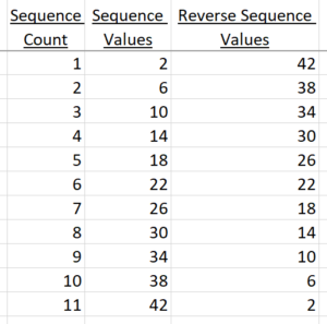
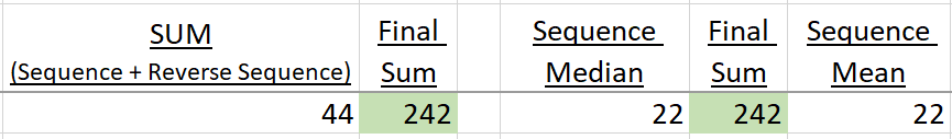
These are the values: 2, 6, 10, 14, 18, 22, 26, 30, 34, 38, 42. SUM is 242 and MEDIAN is 22.

Long sequences were very difficult even for mathematicians before calculators and computers.

Sequences in Excel

It’s easy to create sequences in Excel. (Excel file: save to computer and then open).

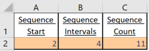
These are the inputs.

Below is a non dynamic array solution that is backwards compatible.

And finally the calculations:

1 Formula Solution

My solution above contains several steps. Let’s create sequence values from a single formula!

Option A

=SEQUENCE(C2,,A2,B2)

=TEXTJOIN(“, “,TRUE,SEQUENCE(C2,,A2,B2))

SEQUENCE is a dynamic array. Requires Office 365 Excel version. TEXTJOIN keeps it from spilling.

Option B

=TEXTJOIN(“, “,TRUE,B2*ROW(INDIRECT(“1:”&C2))-A2)

Formula above is an array and requires Control Shift Enter (just not Enter).

Option C

=B2*ROW(INDIRECT(“1:”&C2))-A2

Formula above doesn’t require Control Shift Enter (just Enter). It spills down into the cells below.

Sequences in Power BI

(download my pbix file.)

GENERATESERIES quickly creates a sequence:

Sequencev1 = GENERATESERIES(2,42,4)

Start with a 2, end at 42, intervals of 4. GENERATESERIES creates a table with 1 column.

Below I use variables but it does the same thing as above. So, is it really necessary?

Sequencev2 =

var SeqCount = 11

var SeqInterval = 4

var SeqStart = 2

var Final = GENERATESERIES(SeqStart,SeqCount*SeqInterval-SeqStart,SeqInterval)

return

Final

Both DAX versions above contain only internal inputs. Could I connect to an input from outside?

After experimenting I created a measure that I referenced when creating a new table.

Here’s the measure:

DistinctProductKeys = DISTINCTCOUNT(FactTable[Product Key])

Here’s the new table that references the measure above:

DynamicSequenceTBL = GENERATESERIES(1,[DistinctProductKeys],1)

If the distinct count changes this viz also updates. GENERATESERIES table function wants 3 single values (start, end, increment). It’s ok for a measure to be the end value. We could use measures for start and increment values as well.

My Dad The Calculator

My dad was really good at math. We would quiz him with multiplication and division questions. He seemed to be able to calculate anything. Hmm…maybe he would also fake some answers knowing that we wouldn’t know the difference.

I don’t think even he could have calculated a simple sum for a long sequence in his head. I bet he would’ve been a big spreadsheet and database fan. I remember that in the mid 1970s my older cousin had a calculator and it was a big deal. Around 1980 I went with my dad to visit his lawyer. He had one of those classic server room computers. I found it fascinating but it probably was less powerful than a smartphone from today.

What’s next? Imagine what things will be like forty years from now. Today’s technology will be ancient.

About Me

My name is Kevin Lehrbass. I live in Markham (near Toronto) Ontario Canada.

I’ve been working with data for almost 20 years now. SQL (various databases), Excel and now Power BI (DAX).

I find it all so interesting that I also have this blog 🙂

Источник

Автозаполнение ячеек в Excel однотипными данными — одна из популярнейших «фишек» этого табличного редактора. Этот простейший процесс — когда вы вводите два числа, а затем просто протягиваете выделение насколько нужно, а программа автоматически заполняет столбец или строку следующими цифрами (датами, буквами и т.п.) идущими по порядку, сэкономил нам столько времени на ввод, что и подумать страшно!

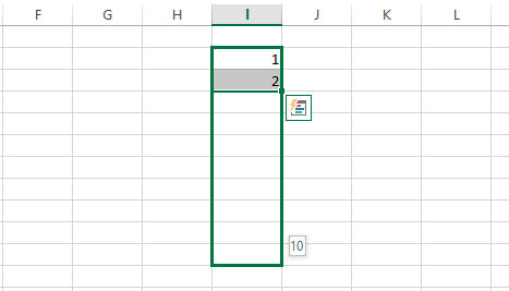
Простейшая арифметическая прогрессия в excel — ввести два первых числа прогрессии (чтобы установить шаг), выделить их, и протащить мышью правый нижний угол выделения до нужной строки

Если записать в соседние ячейки числа, например 1 и 2, то в следующих ячейках появятся значения 4, 5, 6, если записать 500 и 1000, следующими числами будут 1500, 2000 и т.д.

Оба этих числовых ряда будут простейшими арифметическими прогрессиями с заданным шагом — в первом случае с шагом 1, во втором — с шагом 500.

Но, что если мы имеем дело не с простейшей арифметической, а с геометрической прогрессией?

Нет никаких проблем. Введите начальное число в одну из ячеек, а затем выделите диапазон ячеек, в котором и хотите увидеть свою прогрессию.

Инструмент для построения сложных прогрессий в MS Excel

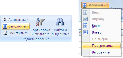
На вкладке «Главная» в группе «Редактирование» найдите инструмент «Заполнить» и выберите пункт «Прогрессия».

В открывшемся окне установите нужные параметры (шаг прогрессии, тип прогрессии и предельное значение, если необходимо), а затем жмите «Ок».

Выбранная вами прогрессия будет мгновенно выведена в пределах выделенного вами диапазона на листе табличного редактора.

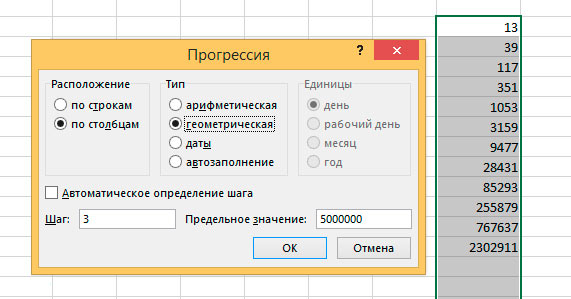
Пример построения геометрической прогрессии с шагом равным 3 и максимальным числом ограниченным 5000000

Также вас может заинтересовать:

Источник

Изучим как сделать арифметическую и геометрическую прогрессии в Excel, а также в общем случае рассмотрим способы создания числовых последовательностей.

Перед построением последовательностей и различных прогрессий, как обычно, вспомним их детальные определения.
Числовая последовательность — это упорядоченный набор произвольных чисел a₁, a₂, a₃, …, a_n, … .
Арифметической прогрессией называется такая числовая последовательность, в которой каждый член, начиная со второго, получается из предыдущего добавлением постоянной величины d (также называют шагом или разностью):

Геометрическая прогрессия — это последовательность чисел, в котором каждый член, начиная со второго, получается умножением предыдущего члена на ненулевое число q (также называют знаменателем):

С определениями закончили, теперь самое время перейти от теории к практике.

Рассмотрим 2 способа задания прогрессии в Excel — с помощью стандартного инструмента Прогрессия и через формулы.
В первом случае на панели вкладок выбираем Главная -> Редактирование -> Заполнить -> Прогрессия:

Далее мы увидим диалоговое окно с настройками параметров:

В данных настройках мы можем выбрать дополнительные параметры, которые позволят нам более детально настроить и заполнить прогрессию в Excel:

Расположение — расположение заполнения (по столбцам или строкам);
Тип — тип (арифметическая, геометрическая, даты и автозаполнение);
Единицы — вид данных (при выборе даты в качестве типа);
Шаг — шаг (для арифметической) или знаменатель (для геометрической);
Автоматическое определение шага — автоматическое определение шага, если заданы несколько значений последовательности;
Предельное значение — ограничение по значению последнего элемента последовательности.

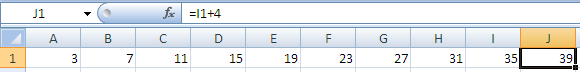
Разберем как сделать арифметическую прогрессию в Excel на конкретном примере.

Создадим набор чисел 3, 7, 11, … , то есть первый элемент равняется 3, а шаг равен 4.
Выделяем диапазон (к примеру, A1:J1) в котором мы хотим разместить набор чисел (диапазон можно и не выделять, однако в этом случае в настройках будет необходимо указать предельное значение), где в первой ячейке будет указан первый элемент (в нашем примере это 3 в ячейке A1), и указываем параметры (расположение, тип, шаг и т.д.):

В результате мы получим заполненный диапазон с заданным набором чисел:

Аналогичный результат можно получить и при задании элементов с помощью формул.
Для этого также задаем начальный элемент в первой ячейке, а в последующих ячейках указываем рекуррентную формулу члена арифметической прогрессии (то есть текущий член получается как сумма предыдущего и шага):

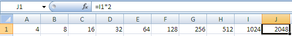
Геометрическая прогрессия в Excel

Принцип построения геометрической прогрессии в Excel аналогичен разобранному выше построению арифметической.
Единственное отличие — в настройках характеристик указываем в качестве типа геометрическую прогрессию.

Например, создадим набор чисел 4, 8, 16, … , то есть первое число равно 4, а каждое последующее в 2 раза больше предыдущего.
Также задаем начальный элемент (4 в ячейке A1), выделяем диапазон данных (например, A1:J1) и указываем параметры:

В итоге получаем:

Идентичного результата также можно добиться и через использование формул:

Числовая последовательность в Excel

Арифметическая и геометрическая прогрессии являются частными случаями числовой последовательности, в общем же случае ее можно создать, как минимум, тремя способами:

Непосредственное (прямое) перечисление элементов;
Через общую формулу n-го члена;
С помощью рекуррентного соотношения, которое выражает произвольный член через предыдущие.

Первый способ подразумевает под собой ручной ввод значений в ячейки. Удобный вариант при вводе небольшого количества значений, в обратном же случае данный способ достаточно трудозатратный.
Второй и третий способы более универсальны, так как позволяют автоматически посчитать значения членов с помощью формул, что удобно при большом количестве элементов.
Поэтому поподробнее остановимся на построении последовательностей данными способами.

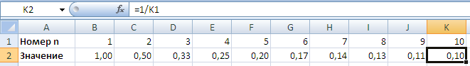
Рассмотрим создание числовой последовательности на примере построения обратных чисел к натуральным, то есть набора чисел 1, 1/2, 1/3, … , в котором общая формула n-го члена принимает вид F_n=1/n.
Создадим дополнительный ряд в отдельной строчке, куда для удобства расчета поместим порядковые номера (1, 2, 3 и т.д.), на которые будут ссылаться формулы:

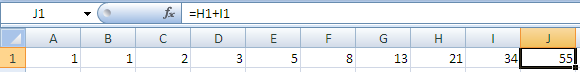
В варианте с рекуррентной формулой рассмотрим пример с набором чисел Фибоначчи, в котором первые два числа равны 1 и 1, а каждый последующее число равно сумме двух предыдущих.
В итоге произвольный член можно представить в виде рекуррентного соотношения F_n = F_n-1 + F_n-2 при n > 2.
Определяем начальные элементы (две единицы) в двух ячейках, а остальные задаем с помощью формулы:

Удачи вам и до скорых встреч на страницах блога Tutorexcel.ru!

Поделиться с друзьями:

Поиск по сайту:

Источник

Инструмент Прогрессия дарит нам несколько замечательных возможностей. С помощью него можно заполнить диапазон ячеек данными по определенному закону: в арифметической или геометрической прогрессии. Для этого не нужно даже знать формулы. Для значений в формате дат предусмотрено создание специфических последовательностей.

Инструмент Прогрессия доступен через меню

Для начала работы введите начальное значение (первый член) прогрессии. Затем выделите диапазон ячеек, куда будут вводиться данные, и вызовите инструмент.

Числовые последовательности

Арифметическая прогрессия представляет собой

числовую последовательность

, где каждое число больше (или меньше) предыдущего на одно и тоже значение (шаг).

Примеры:

Арифметическая прогрессия с шагом 2 — это последовательность чисел 1, 3, 5, 7, 9, 11, … В окне инструмента

Прогрессия

нужно выбрать

Арифметическая

и установить

Шаг

равным 2.

Геометрическая прогрессия с шагом 2 — это последовательность чисел 2, 4, 8, 16, …. Этот пример позволяет быстро вспомнить степени 2. В окне инструмента

Прогрессия

нужно выбрать

Геометрическая

и установить

Шаг

равным 2.

Конечно, арифметическую прогрессию 1, 3, 5, 7, 9, 11, … можно организовать путем формулы

=А1+2

, а геометрическую 2, 4, 8, 16, … —

=А1*2

. Это уже как кому удобнее.

Последовательности дат и рабочих дней

В инструменте

Прогрессия

есть одна замечательная возможность по заполнению значений в формате дат. Вводим дату, выбираем диапазон,

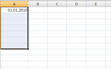
вызываем инструмент

Прогрессия

, выбираем Тип

Даты

, выбираем Единицы

Рабочий день

.

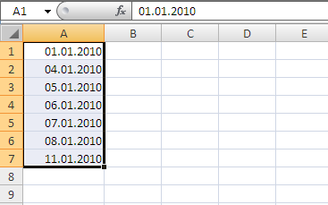
В итоге получаем диапазон, заполненный только одними

рабочими днями

(не суббота и не воскресенье).

Если выберем в качестве единиц месяц, то месяц будет прибавляться к начальной дате и т.д. Эти возможности уже за несколько секунд не реализуешь, нужно вспоминать формулы. А если вспомнить, что еще можно и шаг прогрессии задавать, то можно гарантировать, что формула простой не получится.

Источник

Code:

=sumproduct(b14:b32*(mod(row(b14:b32)-row(b14),6)=0))

shg

MrExcel MVP

If you have n terms of an arithmetic series whose first value is a1 and the constant difference is d, then the sum is

=n*a + n*(n-1)*d/2

it didn’t work
I think you dint understand me !
I want to sum a specific cells which they are making an arithmetic progression (unlimited cells)
as :b14,b20, b26, b32 …….

shg

MrExcel MVP

You don’t need all of the cells, you only need the first cell, the difference, and the number of cells:

	A	B
1	14	A1: Input
2	20	A2: =A1+6
3	26	A3: =A2+6
4	32	A4: =A3+6
5	38	A5: =A4+6
6	44	A6: =A5+6
7	50	A7: =A6+6
8	56	A8: =A7+6
9
10	280	A10: =SUM(A1:A8)
11	280	A11: =8A1 + 8(8-1)*6/2

EDIT: Perhaps I misunderstood; if you want to sum every Nth cell, then use VBA Geek’s formula.

	A	B
1	1
2	8	=A1+A3+A5+A7+A9 ..
3	3
4	5
5	0
6	9
7	7

Like in this table , I want to sum A1+A3+A5+A7+……… Can I write a function to do this calculate ?

The 6 in my formula will determine how many rows to skip

Code:

=sumproduct(b14:b32*(mod(row(b14:b32)-row(b14),[B]6[/B])=0))

so in the above case each 6 rows are summed up, in your last case you need to replace 6 with 2 and also update the B14:B32 reference to A1:A17

shg

MrExcel MVP

If you just want to specify the three values,

	A	B	C	D	E
1	1		Beg	2
2	2		Step	3
3	3		Qty	4
4	4			26	D4: =SUMPRODUCT(INDEX(A:A, Beg):INDEX(A:A, Beg + Step * (Qty — 1)), —(MOD(ROW(INDEX(A:A, Beg):INDEX(A:A, Beg + Step * (Qty — 1))) — Beg, Step) = 0))
5	5
6	6
7	7
8	8
9	9
10	10
11	11
12	12

The 6 in my formula will determine how many rows to skip
Code:
=sumproduct(b14:b32*(mod(row(b14:b32)-row(b14),[B]6[/B])=0))
so in the above case each 6 rows are summed up, in your last case you need to replace 6 with 2 and also update the B14:B32 reference to A1:A17

this one is a solution of my question, I didn’t understand I but thank you
Can you explain it please !

Last edited: May 24, 2014

Источник

Jan 11, 2009

Is it possible to create a formula that would give the sum of cells that are in arithmetic progression in excel?

Example:
Let’s first choose 4 cells that are in arithmetic progression, B14 , B20 , B26 and B32 for instance(the common difference here is 6). So what I want to do is: I want to type a formula in another cell, lets suppose C5, that will automatically give me the sum of the values of B14,B20,B26 and B32. I am aware that I can just type on C5 =B14+B20+B26+B32 but and if I wanted the sum of 90 cells? Wouldn’t it be too much work to type all the cells? Does Anyone know a formula for it?

View 10 Replies

Geometric Progression Function

Dec 29, 2009

I have a range A1:A20 where entering values. I need a function to go true the range and multiple in geometric progression all numbers, if any. ( number of cells with value may range)

View 4 Replies
View Related

Graph Of Progression — Yearly Report

Jul 16, 2014

I have a set of 4 values that I would like to show in a graph. The values I need graphed are as follows:

Brought Forward = 3
New Requests = 2
Closed Requests = 4
Remaining = 1

These 4 numbers will be part of a monthly report (so I only need the numbers graphed once) and also a yearly report (so I would need to find a way to graph all 12 months).

View 1 Replies
View Related

Macro To Display Status Progression With Percentage

May 18, 2014

Display progress bar with percentage completion.

The below code just display macro is running without notifying user the percentage of completion.

[Code] …..

View 2 Replies
View Related

Measure Progression Of A Cell That Is In Dropdown In Excel

Nov 3, 2011

I want to be able to measure the progression of a cell that is in a dropdown in Excel. Once the cell «closes» it is important but it is more important to see what the cell was before it was coded as closed. Is there a way to see what the last item in that cell was? maybe put it in another cell?

View 3 Replies
View Related

Time Arithmetic

Apr 13, 2007

I have a cell (G11) whose format is [h]:mm to store hours worked in a week.
I need to use that in a VBA function. If I query G11.value I get a non-integer number (I DO know that Excel stores time internall like that). How can I get in a VBA procedure exactly what is see in the cell..e.g if someone worked 35:15 hours, I want to be able to get 35:15 in the procedure. I need to strip it from there to work out payment, eg (hourly rate * 35) + (hourly rate * (15/60)/100).

I have tried using format but it does not like the «[h].mm» argument.

View 4 Replies
View Related

Kids Arithmetic

May 9, 2007

I’m trying to put a simple spreadsheet together that will help my son practice
his arithmetic for primary school.

What I have put together is something which will allow him to change say his multiplication tables fairly easily by changing one number.

Conditional formatting shows green if correct and red if wrong — all very easy.

However I think it would be good to show the selected problem in a top down layout
so he can visually see what he is trying to do rather than read across the page.

4
x 2
==
8

rather than 4 x 2 = 8

What I would like to do is change this displayed problem when selects the answer cell
he is working on.

I will attach what I have done so far with a display example on the multiplication tab.

View 9 Replies
View Related

Cell Column Name Arithmetic

Apr 19, 2007

is it possible, in a function, to do something like this?

Lets say I’m in cell N7, and here’s its formula:

IF (N6=$A$13,(A+1)$13,0)

-if the cell before it (N6) is equal to the value of $A$13, then I want N7 to equal the value of B13. If N6 is not equal to $A$13, then place a 0 in cell N7.

basically, I would like to tell my function to move to the next column if it meets a condition in an «IF» statement. Such as, go from column A to Column B given a certain condition. Otherwise, stay in column A until that condition is met.

View 9 Replies
View Related

Timesheets — Time Arithmetic

Jan 30, 2009

I have a timesheet in excel which details the hours worked per person. It is worked out by have time started in one cell, and time finished in the next cell. (24 hour clock).

The timesheet is for a night club, so people start late, and finish early. Therfore, in the total column I have the following formula…

=IF(D5=»»,0,IF(D5

View 9 Replies
View Related

Arithmetic Operator From Cell Reference

Jul 23, 2014

I need to switch between less than or greater than in my formula based on user selected drop down that gives the user two options «» My formula has «

View 9 Replies
View Related

Time Arithmetic — Calculate Hour Difference

Apr 10, 2014

Time arithmetic, I have two cells representing a time range.

The first one (say: X1) is formatted using the custom format [h]:mm and contains a certain number of hours and minutes. It gets its value by summing up other cells in the same format. A typical entry could be 98:35 to represent a duration 98 hours and 35 minutes.

The second cell (say: X2) is formatted as a number with 4 decimal places after the comma, and similarily gets its value by summing up other cells in the same format. It also represents a time duration as a number of hours. A typical entry could be 202.7500 to represent a duration of 202 hours and 45 minutes (because 0.75 of an hour is 45 minutes).

I would like to calculate the hour difference between these cells, and display it as hours and minutes. In the example given, the result should be negative, i.e. -104:10.

My first approach was to use the formula X1-X2 and format the result as [h]:mm, but this gives me a #VALUE! error.

View 2 Replies
View Related

Extract Numbers From String And Run Arithmetic Function Using Excel VBA

Aug 6, 2012

I have a column A with following values below:

Column A
«VL50s»
«M50s»
«H50s»
«VL50s»
«H50s»

I would like to extract the numbers and run the following arithmetic function below into column B.

key:
x is a number
VLx —> (x) + 1
Mx —>(x) + 2
Hx —> (x) + 3

the output should look like the following using the key above:

column B
51
52
53
51
53

View 9 Replies
View Related

Excel 2007 :: Use Dates As Argument In Boolean Arithmetic?

Nov 22, 2013

Can I use dates as argument in Boolean arithmetic? I have a list of name with their date of birth and I would like to tell who is between 18 and 25. It’s easy enough with number but with dates? Excel 2007

View 9 Replies
View Related

Excel 2013 :: Simple Date Arithmetic — Circular Reference?

Aug 10, 2014

Here is a very simple workbook/sheet with some simple date arithmetic.

I keep getting the warning that there’s a circular reference in C2.

Either I need to suppress the warning so vba loops can run or PREFERABLY I’d get rid of the «circular reference».

Run with Excel 2013.

View 14 Replies
View Related

GeoCode Arithmetic: MapsCo Grid To «overlay» GeoLoc Data

Mar 23, 2009

I’m trying to come up with a MapsCo grid to «overlay» geoLoc data. Given the coordinates of a single box within a MapsCo page, I’ll can figure out the others once I know how to «from this point, add .5 miles due North and mark another point; from that point, add .5 miles due East and record the next point; etc».

View 5 Replies
View Related

Linking Cells Globally To Allow Users Ability To Change Cells On Separate Sheet / Cells?

Feb 18, 2014

I have a workbook that uses the values that a user had entered into 3 cells to calculate multiple other charts/diagrams on multiple sheets within the workbook. Each sheet would show what the user had entered in the 3 cells to allow them to see what is being used to calculate each table. Is it possible to link these cells so that the user can change the 3 values without having to go back to where he originally entered the 3 values?

For example, a user has entered in 3 values in Sheet 1. A formula in Sheet 2 displays what is entered by the user and uses these calls in Sheet 2 for calculations. When the user wants to change the three values, he would have to navigate to Sheet 1 and enter in the new values to have the workbook recalculate all the tables. Is there a way to link the three cells from Sheet 1 and Sheet 2 so when the user is on Sheet 2, he has the opportunity to change the values on the current Sheet without having to navigate to Sheet 1 to do so?

View 1 Replies
View Related

Copying Merged Cells (3 Cells) Based On Contents Of Any Of 3 Cells To Right

May 29, 2014

I wish to copy a merged cell (3 cells) based on if only 1 of 3 cells to the right contain «X». if the top cell does not contain «X» than the merged cell is not copied. Also, is therea more elegant to copy 3 columns at a time rather than do one at a time as my code shows:

Sub CopyICUCAPU()
‘
‘ CopyICUCAPU Macro
‘
Dim i As Integer

[Code]…..

View 14 Replies
View Related

Values In Each Cells(A) Represented Back At Cells(B) But No Repetition If Some Cells(A) Contains Same Value

Dec 9, 2008

I did my search, but cant find and knows what key search to look/type for…

If i have data A1 through A10, such as 1 1 2 2 2 2 3 3 3 3

How can i get column B1 through B3 as 1 2 3 ?

View 9 Replies
View Related

Date Cells In Project Plan To Change Based On Other Cells Including Other Date Cells

Oct 31, 2008

This is a project plan with tasks and dates. Column A is the activity number. (Example 1, 2, 3″ etc). Column B is the task (Ex. «Complete Report»). Column C is number of days required to complete the task. Column D is the dependency column. (Ex. Cell D2 =1 in other words Task 2 is dependent on task 1). Column E is the date.

I would like to have a seperate start date cell and a go live date cell.

The objective is to enter a start date, and have each column E date increase based on the number of days entered in Column C. If a task is dependent on another and I change the number of days in Column C I need the dependent task to change the same amount of days.

View 9 Replies
View Related

How To Copy Row With Formula In Locked Cells And Insert Copied Cells In Protected Sheet

Mar 29, 2014

Have you ever copy a row with formula in locked cells & insert it in a protected worksheet?

View 1 Replies
View Related

Lookup Range Of Cells And Populate Specific Cells Based On Matching Data?

May 23, 2014

I am trying to build a staff roster. The staff rotate over a 4 week cycle. the name of the staff member, and their shift needs to be looked up from the key then matched with the particular week. the name and shift then need to populate specific cells.

I have attached the worksheet so you can see what i am trying to achieve.

View 2 Replies
View Related

Copy Filter Data And Paste It On Another Workbook With Special Cells (Only Visible Cells)

Apr 12, 2014

I am using code to filter my 4 sheets Greater then 0 (zero)

After apply above filter now i need to copy multiple rows and paste on another specific workbook for paste i m using below code:

for 1st sheet with the name («V2»)

for 2nd sheet with the name(«LV»)

For 3rd sheet with the name («F2»)

and 4th sheet with the name(«L2»)

If I play above code one by one all is going very well,,,,,,or if use in this way all is going very well

But here is a big problem……….if any sheet have no value greater then 0(zero)….then code paste all data… e.g shssts(«LV») .Range(«C5:C54»).Copy but C5:C54 have no data greater then 0(zero) and it will paste on another sheet c5:c54 and again new sheets data will paste below the c54 while c5:c54 have no data.

So I want if any sheet have no data with range is greater then 0(Zero) then skip the copy paste code or use like SpecialCells(xlCellTypeVisible) .

View 5 Replies
View Related

Protect Certain Locked Cells From Editing And Allow Certain Unlocked Cells To Be Changed On Multiple Worksheets?

Jan 31, 2014

1.I need to protect certain locked cells from editing and allow certain unlocked cells to be changed on multiple worksheets.

2.When all of the changes are made to the unlocked cells, I need to password protect the entire workbook (except one worksheet) from any changes. (i.e. Prevent even the unlocked cells from being edited)

3.I also need a password to un-protect the workbook and return it to the state described in # 1. above .

View 1 Replies
View Related

Excel 2007 :: Conditional Formatting Empty Cells Based On Full Cells?

Nov 17, 2011

Working in Excel 2007. I am using excel for a data log (basically) and want it to format all empty cells in a row yellow if there is data in column A

Basically, If i have a value in A2, I want any empty cell between B2-G2 to be filled in yellow (as an idicator to the inputter that the cell needs to be completed).

there is already conditional formatting on these cells, which i want to maintain for the non-empty cells. I also have «0» as a value, so I couldn’t use the basic conditional formatting setting it =0, it highlighted cells with $0.00, which i do not want.

View 5 Replies
View Related

Excel 2003 :: Conditional Format Top / Mid / Bottom 33% Of Cells But Ignoring Blank Cells

Mar 25, 2012

I am trying to conditionally format the top middle and bottom thirds of a range of data. Problem is, that the range needs to be flexible as sometimes there may be a maximum of 36 cells with data, but sometimes there may be less (so there are blank cells in the range that need not be counted). The methods I have tried always include the blank cells, and so it is not equally formatting the thirds (as it includes the blanks cells as part of the bottom data)….

Here are the 2 methods Ive tried so far using excel 2003)
Top 34%:
=IF(INT(COUNT($D$3:$D$38)*34%)>0,LARGE($D$3:$D$38,INT(COUNT($D$3:$D
$38)*34%)),MAX( $D$3:$D$38))0,LARGE($D$3:$D$38,INT(COUNT($D$3:$D
$38)*67%)),MAX( $D$3:$D$38))0,LARGE($D$3:$D$38,INT(COUNT($D$3:$D
$38)*100%)),MAX( $D$3:$D$38))

View 4 Replies
View Related

Excel 2010 :: Color Fill A Range Of Cells If Specific Cells Not Blank

Feb 7, 2013

I am using Excel 2010 and basically i am trying to fill a range of cell with a green color if any value was enter in a specific cells. Example: I would like to fill range: A10:c13 with a green color (regardless of the cells content in this range) if a value was entered in cell C10 or C11 or C12 or C13.

I’ve tried conditional formatting but unfortunately I’ll have to apply formatting for every cell and for a range of over hundred cells is not efficient.

View 7 Replies
View Related

Locking Text In Cells But Not The Ability To Change Colour Of Cells With Mouse Click

Mar 5, 2013

Locking text in cells but not the ability to change colour of cells

******** width=»234″ height=»60″ frameborder=»0″ marginwidth=»0″
marginheight=»0″ vspace=»0″ hspace=»0″ allowtransparency=»true» scrolling=»no» id=»aswift_0″ name=»aswift_0″ style=»left: 0px; position: absolute; top: 0px;»>*********>

I have a spreadsheet where I can change the colour of a cell by clicking the mouse, I also have text in many of the cells.

What I need to do is protect (lock) the text so that no one can change the text in any of the cells, but I still want to be able to change the colour of the cells by clicking the mouse in that cell.

View 2 Replies
View Related

Sort Rows To Show Values Of Cells In Sequence And Eliminate Empty Cells

Nov 11, 2013

I have data on 400 rows. Each row has a maximum of 10 cells with data, but many have empty cells with no data. I would like to sort each row to show values of cells in sequence and eliminate empty cells. I can use the sort row function but its a long process for 400 individual rows. Is there an easier way?

View 1 Replies
View Related

Conditional Format Cells Containing Numbers And Letters — Ignore Cells With Number Only

Jul 11, 2014

I have a column of numbers and want to make sure everything has been entered correctly from our scanning software. Basically, I want to automatically highlight any cell that has any letter in it (e.g. z12o2 instead of 21202 or R705 instead of 5705), ignoring any cells that contain only numbers. I haven’t had any luck using conditions based on formulas like =ISTEXT.

View 2 Replies
View Related

Count Cells Containing Dates (greater Than 2014) Based On Filtered Cells

Jun 24, 2014

I have spreadsheet with different 100s of columns of dates with 600 rows. The first row identifies which zone the data belongs to (North, South, East, West. NE, SW, SW1, etc…)

I want to write a formula to check how many dates in each column fall in 2015 or later years; This can be accomplished by writing a countifs formula.

Where it gets complicated is once i filter on the Zones;

I want the formula to give me the desired result — count of all CELLS where the year is 2015 or greater — WITH FILTERS ON.

I stumbled upon following sumproduct formula that gives count for visible cells, however when i apply the date criteria, i get incorrect result —

=SUMPRODUCT(SUBTOTAL(3,OFFSET(IJ3:IJ999,ROW(IJ3:IJ999)-MIN(ROW(IJ1:IJ999)),,1))*(IJ3:IJ999>DATE(2014,12,31)))

View 8 Replies
View Related

Источник

01-11-2009, 04:43 PM

#1

Registered User

Arithmetic Progression with cells?

Hi!
My question is : Is it possible to create a formula that would give the sum of cells that are in arithmetic progression in excel?

Example:
Let’s first choose 4 cells that are in arithmetic progression, B14 , B20 , B26 and B32 for instance(the common difference here is 6). So what I want to do is: I want to type a formula in another cell, lets suppose C5, that will automatically give me the sum of the values of B14,B20,B26 and B32. I am aware that I can just type on C5 =B14+B20+B26+B32 but and if I wanted the sum of 90 cells??Wouldn’t it be too much work to type all the cells? Does Anyone know a formula for it?

thanks! :]

Last edited by Golden02; 01-11-2009 at 09:17 PM.
01-11-2009, 04:58 PM

#2

If you have an arithmetic series in A1, A2, …, then the sum of the first N terms in the series is=N*(2*A1 + (N-1)*(A2-A1)) / 2

Entia non sunt multiplicanda sine necessitate
01-11-2009, 05:42 PM

#3

Registered User

Originally Posted by shg

If you have an arithmetic series in A1, A2, …, then the sum of the first N terms in the series is

=N*(2*A1 + (N-1)*(A2-A1)) / 2

Hmmm, I get it, thanks for the formula. But what I mean is, it is not the value of A1 , A2, …, AN that is in arithmetic series, what is in arithmetic series is the cells themselves. It is like if:
C20 = 550
C25 = 10
C30 = 200
Their values are not in arithmetic series but they are. Can you see that C30 is 5 rows away from C25 and C25 is also 5 rows away from C20?
Is there any formula for the sum of these cells?
thanks again
01-11-2009, 05:47 PM

#4

Their values are not in arithmetic series but they are.

I can’t parse that.

Can you see that C30 is 5 rows away from C25 and C25 is also 5 rows away from C20?

Yes … so?
01-11-2009, 06:02 PM

#5

C20 = 550
C25 = 10
C30 = 200

Dos that mean you want to sum 200 cells in column B, starting at B550, and adding every 10th cell?
01-11-2009, 06:15 PM

#6

Registered User

Originally Posted by shg

I can’t parse that.

Yes … so?

Hmmm let me try to explain it to you.
I want to calculate the sum of cells that have their LOCATION as an arithmetic progression.
What I mean by location is the row and the column that each is.
Take a close look at the number of the rows from the cells C20 C25 and C30:
20 , 25 , 30 can you picture that these numbers are in arithmetical series?
So I thought that it might be possible to calculate the sum of cells that would have their rows as an arithmetic series.
Do you get my idea?
01-11-2009, 06:22 PM

#7

OK; so what cells should be summed for that example?
01-11-2009, 06:29 PM

#8

Registered User

For that example C20 , C25 and C30
If I want to sum them in T4, I just have to type there =C20+C25+C30 right?
But this is easy because we are talking about 3 cells.
And If I wanted to sum 50 cells just knowing that the number of their rows is always increasing by 5?
Like C20 , C25 , C30 , …, C255
You get that?
01-11-2009, 06:37 PM

#9

Last edited by shg; 01-11-2009 at 08:27 PM.
01-11-2009, 06:57 PM

#10

Registered User

Exactly like this!!
To be honest, I really didn’t understand the formula you used to calculate it. But I understood how you did it.

I think that that solves my problem :D!
thank you very much for the help

PS: I’ll try to use it right now.

Last edited by shg; 01-11-2009 at 08:29 PM.

Reason: deleted spurious quote
01-11-2009, 08:26 PM

#11

You’re welcome. Would you please mark the thread as Solved?

Click the Edit button on your first post in the thread

Click Go Advanced, select [SOLVED] from the Prefix dropdown, then click Save Changes

Please don’t quote whole posts — it just clutters the forum.

I updated my last post to show the formula in D4.

Last edited by shg; 01-11-2009 at 08:29 PM.
03-24-2013, 05:19 AM

#12

Registered User

Re: Arithmetic Progression with cells?

I apologize for the necro, but I followed shg‘s example exactly and got 1088 as the sum instead of 277…

Since I don’t know see an attachment option, I only include the screenshot of it (even though it’s meaningless):
1

Could someone please tell me what I’ve missed out here?

Источник

Using AutoFill in Excel, you can quickly fill the same sequence or the sequence with a tolerance of 1 directly. But what if the tolerance of arithmetic sequence you need to fill is not 1? In fact, Excel enables you to customize the tolerance and fill the arithmetic sequence automatically. Let’s see how to do it.

1. Open an Excel sheet, enter the initial value in any of the cells.

2. Select all the cells you want to fill in the arithmetic sequence.

3. Find Fill button in Home tab. Choose Series… in the drop-down list.

4. Check Linear in Type and enter the tolerance beside Step value. Then hit OK to implement it.

5. Now the arithmetic sequence is filled automatically.

6. You can also enter a negative nubmer in Step value.

7. Thus you can fill a decreasing arithmetic sequence quickly.

Copyright Statement: Regarding all of the posts by this website, any copy or use shall get the written permission or authorization from Myofficetricks.

Источник

Probably everyone can summarize data in Excel program. But with the improved version of the SUM function, which is called SUMIF, the capabilities of this operation are significantly expanded.

By the name of the function, you can understand that it does not only calculate the sum, but also complies with some logical conditions.

SUMIF and its syntax

The SUMIF function allows you to sum cells that meet a certain criterion (a given condition). The arguments of the function are as follows:

SUMIF.

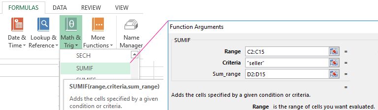
Range — cells, which should be evaluated on the basis of the criterion (the specified condition).
Criteria, determining which cells from the range will be selected (written in quotation marks).
Sum range — the actual cells that are needed to be summed if they meet the criterion.

Consequently the function has only 3 arguments. However, sometimes the third one can be excluded, and then the command will work only by the range and criteria.

How does the SUMIF function work in Excel?

Let’s consider the simplest example, which will clearly demonstrate how to use the SUMIF function and how convenient it can be for solving certain tasks.

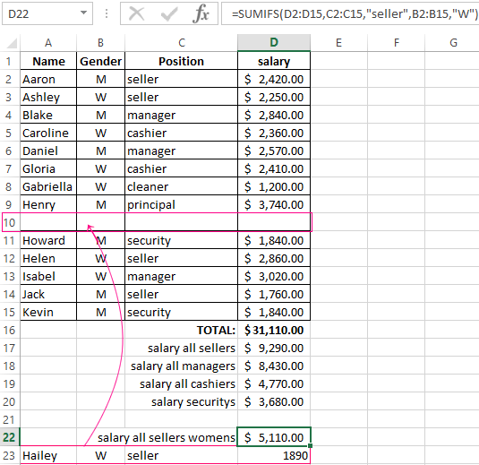
We have a table in which the names of employees, their gender and salary, calculated for January are indicated. If we just need to calculate the total amount of money that is required to pay out to employees, we use the SUM function, specifying all salaries by the range.

But what do we have to do if we need to quickly calculate only sellers’ salaries? In this case, the use of the SUMIF function will help.

Enter the arguments.

The range in this case will be a list of all staff posts, because we will need to determine the whole amount of salaries. Therefore, enter E2:E14.
The criterion of choice in our case is the seller. Enclose the word in quotation marks and put it as the second argument.
The range of summation is salaries, because we need to know the amount of salaries of all sellers. Therefore, enter F2:F14.

Done.

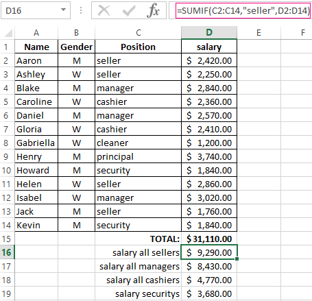
We have obtained 9290$. It means that the function automatically elaborated the list of all posts, chose only sellers from them and summed up their salaries.

Similarly, you can calculate the salaries of all managers, vendors, cashiers and security guards. When the table is small, it seems that everything can be counted manually, but when working with lists having several hundreds of positions, it makes sense to use SUMIF function.

SUMIF function in Excel with multiple criteria SUMIFS

If the letter S is added to the end of the standard SUMIF command, then it implies the function with several criteria (SUMIFS function). It is used in the case when you need to specify more than one criterion.

Syntax of using the function by several criteria

There can be as many arguments for SUMIFS as you like, but no less than 5.

SUMIFS.

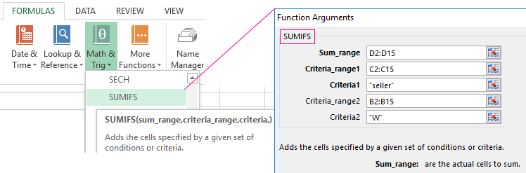
Sum range. If in SUMIF it was at the end, then here it is in the first place. It also indicates the cells that need to be summed.
Criteria range 1 — cells that need to be evaluated on the basis of the first criterion.
Criteria 1 — defines the cells that the function will select from the first range of the condition.
Criteria range 2 — cells, which should be evaluated on the basis of the second criterion.
Criteria 2 — defines the cells that the function will select from the second condition range.

And so on. Depending on the number of criteria, the number of arguments can increase in an arithmetic progression in step 2. That is, 5, 7, 9 …

Example of use

Suppose we need to calculate the amount of salaries of all female sellers for January. We have two conditions. The employee must be:

a seller;
a woman.

So, we will use the SUMIFS command.

Enter the arguments.

Sum range — cells with a salary;
Criteria range 1 — cells indicating the post of the employee;
Criteria 1 — the seller;
Criteria range 2 — cells with gender of the employee;
Criteria 2 — female (f).

result.

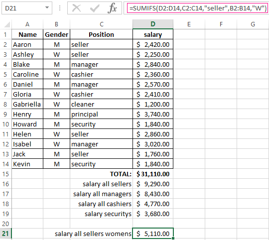
The result: all female sellers in January received in summation 5110$.

SUMIF in Excel with dynamic criterion

The SUMIF and SUMIFS functions are useful because they automatically fit themselves to the changing criteria. That is, we can change the data in cells, and the sums will change with them. For example, when calculating salaries, it turned out that we forgot to take into account one employee who works as a seller. We can add one more line by right-clicking and selecting the ВСТАВИТЬ command.

We have an additional row. We can see that the range of conditions and summations has automatically expanded to 15 rows.

Copy the employee’s data and paste it into the general list. The sums in the resulting cells have changed. The functions have reacted to the appearance of another female seller in the range.

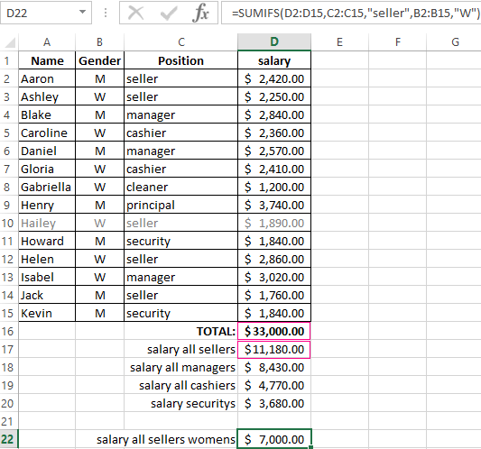
Similarly, you can not only add, but also delete any rows (for example, when the employee is discharged), change the values, etc.

Источник