
Arguments are the values that functions use to perform calculations. In spreadsheet programs such as Excel and Google Sheets, functions are just built-in formulas that carry out set calculations and most of these functions require data to be entered, either by the user or another source, in order to return a result.
Contents
- 1 What is the argument in an Excel function?
- 2 What are arguments in Excel explain giving example?
- 3 What is the type argument in Excel?
- 4 What are the two kinds of arguments in Excel?
- 5 What are the 3 arguments of the IF function?
- 6 How do you create an argument in Excel?
- 7 What is the argument of a story?
- 8 What is an argument in parentheses?
- 9 How many arguments can a function have in Excel?
- 10 What are the 3 types of cell references in Excel?
- 11 What is a syntax in Excel?
- 12 How do you access function arguments in Excel?
- 13 What are the 10 logical functions in Excel?
- 14 How do you create a logical argument in Excel?
- 15 How many arguments are required for the SUM function?
- 16 What is Vlookup in Excel?
- 17 What does spill mean in Excel?
- 18 What is the third argument in an IF statement in Excel?
- 19 What does the rand function do?
- 20 What is argument explain with example?
What is the argument in an Excel function?
A function argument is a specific input to a function. For example, the VLOOKUP function takes four arguments as follows: =VLOOKUP (value, table, col_index, [range_lookup]) Note most arguments are required, but some are optional. In Excel, optional arguments are denoted with square brackets.
What are arguments in Excel explain giving example?
Most of the functions found in Excel require some input or information in order to calculate correctly. For example, to use the AVERAGE function, you need to give it a range of numbers to average. =AVERAGE(A1:A100) Any input you give to a function is called an argument.
What is the type argument in Excel?
The Excel TYPE function returns a numeric code representing “type” in 5 categories: number = 1, text = 2, logical = 4, error = 16, and array = 64. Use TYPE when the operation of a formula depends on the type of value in a particular cell.
What are the two kinds of arguments in Excel?
The types of arguments that are used in Excel are given below.
- Numeric data (=SUM(5,10))
- Text-string data (=UPPER(“siam”))
- Boolean values (=OR(1+1=2))
- Error Values (=ISERR(#VALUE!))
- Other functions (=DATE(YEAR(A2) + B2, MONTH(A2), DAY(A2)))
What are the 3 arguments of the IF function?
There are 3 parts (arguments) to the IF function:
- TEST something, such as the value in a cell.
- Specify what should happen if the test result is TRUE.
- Specify what should happen if the test result is FALSE.
How do you create an argument in Excel?
Follow these steps:
- Click the cell with the existing function.
- Click the Insert Function button. The Function Argument dialog box appears.
- Add, edit, or delete arguments, as follows:
- Click OK when you’re finished.
What is the argument of a story?
Argument Definition
An argument is the main statement of a poem, an essay, a short story, or a novel, which usually appears as an introduction, or a point on which the writer will develop his work in order to convince his readers. Literature does not merely entertain. It also intends to shape the outlook of readers.
What is an argument in parentheses?
1. For the initial line of a Sub or Function, you use parentheses to enclose the arguments (if any), e.g. Sub MySubroutine(a As Long, b As String) or. Function MyFunction(a As Long, B As String) As Long.
How many arguments can a function have in Excel?
The concept of additional optional arguments is expressed with ellipses, which appear at the end of the argument list when a function takes multiple optional arguments. The SUM function can actually accept up to 256 arguments total.
What are the 3 types of cell references in Excel?
Relative, Absolute and Mixed
A key element of a formula is the cell reference, and there are three types: Relative. Absolute. Mixed.
What is a syntax in Excel?
The syntax of a function in Excel or Google Sheets refers to the layout and order of the function and its arguments.All functions begin with the equal sign ( = ) followed by the function’s name such as IF, SUM, COUNT, or ROUND.
How do you access function arguments in Excel?
Keyboard shortcut fans might know that you can start typing a formula, like =VLOOKUP(, into a cell and then press Ctrl+A to open the Functions Argument for that function.
What are the 10 logical functions in Excel?
Excel logical functions – overview
| Function | Description | Formula Example |
|---|---|---|
| AND | Returns TRUE if all of the arguments evaluate to TRUE. | =AND(A2>=10, B2<5) |
| OR | Returns TRUE if any argument evaluates to TRUE. | =OR(A2>=10, B2<5) |
| XOR | Returns a logical Exclusive Or of all arguments. | =XOR(A2>=10, B2<5) |
How do you create a logical argument in Excel?
Use the IF function, one of the logical functions, to return one value if a condition is true and another value if it’s false. For example: =IF(A2>B2,”Over Budget”,”OK”) =IF(A2=B2,B4-A4,””)
Syntax.
| Argument name | Description |
|---|---|
| value_if_false (optional) | The value that you want returned if the result of logical_test is FALSE. |
How many arguments are required for the SUM function?
These values can be numbers, cell references, ranges, arrays, and constants, in any combination. SUM can handle up to 255 individual arguments. The SUM function takes multiple arguments in the form number1, number2, number3, etc. up to 255 total.
What is Vlookup in Excel?
VLOOKUP stands for ‘Vertical Lookup’. It is a function that makes Excel search for a certain value in a column (the so called ‘table array’), in order to return a value from a different column in the same row.
What does spill mean in Excel?
#SPILL errors are returned when a formula returns multiple results, and Excel cannot return the results to the grid.
What is the third argument in an IF statement in Excel?
The IF Function has 3 arguments: Logical test. This is where we can compare data or see if a condition is met. Value if true.
What does the rand function do?
RAND returns an evenly distributed random real number greater than or equal to 0 and less than 1. A new random real number is returned every time the worksheet is calculated. Note: As of Excel 2010, Excel uses the Mersenne Twister algorithm (MT19937) to generate random numbers.
What is argument explain with example?
For example, consider the argument that because bats can fly (premise=true), and all flying creatures are birds (premise=false), therefore bats are birds (conclusion=false). If we assume the premises are true, the conclusion follows necessarily, and it is a valid argument.
If you’re new to Excel for the web, you’ll soon find that it’s more than just a grid in which you enter numbers in columns or rows. Yes, you can use Excel for the web to find totals for a column or row of numbers, but you can also calculate a mortgage payment, solve math or engineering problems, or find a best case scenario based on variable numbers that you plug in.
Excel for the web does this by using formulas in cells. A formula performs calculations or other actions on the data in your worksheet. A formula always starts with an equal sign (=), which can be followed by numbers, math operators (such as a plus or minus sign), and functions, which can really expand the power of a formula.
For example, the following formula multiplies 2 by 3 and then adds 5 to that result to come up with the answer, 11.
=2*3+5
This next formula uses the PMT function to calculate a mortgage payment ($1,073.64), which is based on a 5 percent interest rate (5% divided by 12 months equals the monthly interest rate) over a 30-year period (360 months) for a $200,000 loan:
=PMT(0.05/12,360,200000)
Here are some additional examples of formulas that you can enter in a worksheet.
-
=A1+A2+A3 Adds the values in cells A1, A2, and A3.
-
=SQRT(A1) Uses the SQRT function to return the square root of the value in A1.
-
=TODAY() Returns the current date.
-
=UPPER(«hello») Converts the text «hello» to «HELLO» by using the UPPER worksheet function.
-
=IF(A1>0) Tests the cell A1 to determine if it contains a value greater than 0.
The parts of a formula
A formula can also contain any or all of the following: functions, references, operators, and constants.

1. Functions: The PI() function returns the value of pi: 3.142…
2. References: A2 returns the value in cell A2.
3. Constants: Numbers or text values entered directly into a formula, such as 2.
4. Operators: The ^ (caret) operator raises a number to a power, and the * (asterisk) operator multiplies numbers.
Using constants in formulas
A constant is a value that is not calculated; it always stays the same. For example, the date 10/9/2008, the number 210, and the text «Quarterly Earnings» are all constants. An expression or a value resulting from an expression is not a constant. If you use constants in a formula instead of references to cells (for example, =30+70+110), the result changes only if you modify the formula.
Using calculation operators in formulas
Operators specify the type of calculation that you want to perform on the elements of a formula. There is a default order in which calculations occur (this follows general mathematical rules), but you can change this order by using parentheses.
Types of operators
There are four different types of calculation operators: arithmetic, comparison, text concatenation, and reference.
Arithmetic operators
To perform basic mathematical operations, such as addition, subtraction, multiplication, or division; combine numbers; and produce numeric results, use the following arithmetic operators.
|
Arithmetic operator |
Meaning |
Example |
|
+ (plus sign) |
Addition |
3+3 |
|
– (minus sign) |
Subtraction |
3–1 |
|
* (asterisk) |
Multiplication |
3*3 |
|
/ (forward slash) |
Division |
3/3 |
|
% (percent sign) |
Percent |
20% |
|
^ (caret) |
Exponentiation |
3^2 |
Comparison operators
You can compare two values with the following operators. When two values are compared by using these operators, the result is a logical value — either TRUE or FALSE.
|
Comparison operator |
Meaning |
Example |
|
= (equal sign) |
Equal to |
A1=B1 |
|
> (greater than sign) |
Greater than |
A1>B1 |
|
< (less than sign) |
Less than |
A1<B1 |
|
>= (greater than or equal to sign) |
Greater than or equal to |
A1>=B1 |
|
<= (less than or equal to sign) |
Less than or equal to |
A1<=B1 |
|
<> (not equal to sign) |
Not equal to |
A1<>B1 |
Text concatenation operator
Use the ampersand (&) to concatenate (join) one or more text strings to produce a single piece of text.
|
Text operator |
Meaning |
Example |
|
& (ampersand) |
Connects, or concatenates, two values to produce one continuous text value |
«North»&»wind» results in «Northwind» |
Reference operators
Combine ranges of cells for calculations with the following operators.
|
Reference operator |
Meaning |
Example |
|
: (colon) |
Range operator, which produces one reference to all the cells between two references, including the two references. |
B5:B15 |
|
, (comma) |
Union operator, which combines multiple references into one reference |
SUM(B5:B15,D5:D15) |
|
(space) |
Intersection operator, which produces one reference to cells common to the two references |
B7:D7 C6:C8 |
The order in which Excel for the web performs operations in formulas
In some cases, the order in which a calculation is performed can affect the return value of the formula, so it’s important to understand how the order is determined and how you can change the order to obtain the results you want.
Calculation order
Formulas calculate values in a specific order. A formula always begins with an equal sign (=). Excel for the web interprets the characters that follow the equal sign as a formula. Following the equal sign are the elements to be calculated (the operands), such as constants or cell references. These are separated by calculation operators. Excel for the web calculates the formula from left to right, according to a specific order for each operator in the formula.
Operator precedence
If you combine several operators in a single formula, Excel for the web performs the operations in the order shown in the following table. If a formula contains operators with the same precedence—for example, if a formula contains both a multiplication and division operator— Excel for the web evaluates the operators from left to right.
|
Operator |
Description |
|
: (colon) (single space) , (comma) |
Reference operators |
|
– |
Negation (as in –1) |
|
% |
Percent |
|
^ |
Exponentiation |
|
* and / |
Multiplication and division |
|
+ and – |
Addition and subtraction |
|
& |
Connects two strings of text (concatenation) |
|
= |
Comparison |
Use of parentheses
To change the order of evaluation, enclose in parentheses the part of the formula to be calculated first. For example, the following formula produces 11 because Excel for the web performs multiplication before addition. The formula multiplies 2 by 3 and then adds 5 to the result.
=5+2*3
In contrast, if you use parentheses to change the syntax, Excel for the web adds 5 and 2 together and then multiplies the result by 3 to produce 21.
=(5+2)*3
In the following example, the parentheses that enclose the first part of the formula force Excel for the web to calculate B4+25 first and then divide the result by the sum of the values in cells D5, E5, and F5.
=(B4+25)/SUM(D5:F5)
Using functions and nested functions in formulas
Functions are predefined formulas that perform calculations by using specific values, called arguments, in a particular order, or structure. Functions can be used to perform simple or complex calculations.
The syntax of functions
The following example of the ROUND function rounding off a number in cell A10 illustrates the syntax of a function.
1. Structure. The structure of a function begins with an equal sign (=), followed by the function name, an opening parenthesis, the arguments for the function separated by commas, and a closing parenthesis.
2. Function name. For a list of available functions, click a cell and press SHIFT+F3.
3. Arguments. Arguments can be numbers, text, logical values such as TRUE or FALSE, arrays, error values such as #N/A, or cell references. The argument you designate must produce a valid value for that argument. Arguments can also be constants, formulas, or other functions.
4. Argument tooltip. A tooltip with the syntax and arguments appears as you type the function. For example, type =ROUND( and the tooltip appears. Tooltips appear only for built-in functions.
Entering functions
When you create a formula that contains a function, you can use the Insert Function dialog box to help you enter worksheet functions. As you enter a function into the formula, the Insert Function dialog box displays the name of the function, each of its arguments, a description of the function and each argument, the current result of the function, and the current result of the entire formula.
To make it easier to create and edit formulas and minimize typing and syntax errors, use Formula AutoComplete. After you type an = (equal sign) and beginning letters or a display trigger, Excel for the web displays, below the cell, a dynamic drop-down list of valid functions, arguments, and names that match the letters or trigger. You can then insert an item from the drop-down list into the formula.
Nesting functions
In certain cases, you may need to use a function as one of the arguments of another function. For example, the following formula uses a nested AVERAGE function and compares the result with the value 50.
1. The AVERAGE and SUM functions are nested within the IF function.
Valid returns When a nested function is used as an argument, the nested function must return the same type of value that the argument uses. For example, if the argument returns a TRUE or FALSE value, the nested function must return a TRUE or FALSE value. If the function doesn’t, Excel for the web displays a #VALUE! error value.
Nesting level limits A formula can contain up to seven levels of nested functions. When one function (we’ll call this Function B) is used as an argument in another function (we’ll call this Function A), Function B acts as a second-level function. For example, the AVERAGE function and the SUM function are both second-level functions if they are used as arguments of the IF function. A function nested within the nested AVERAGE function is then a third-level function, and so on.
Using references in formulas
A reference identifies a cell or a range of cells on a worksheet, and tells Excel for the web where to look for the values or data you want to use in a formula. You can use references to use data contained in different parts of a worksheet in one formula or use the value from one cell in several formulas. You can also refer to cells on other sheets in the same workbook, and to other workbooks. References to cells in other workbooks are called links or external references.
The A1 reference style
The default reference style By default, Excel for the web uses the A1 reference style, which refers to columns with letters (A through XFD, for a total of 16,384 columns) and refers to rows with numbers (1 through 1,048,576). These letters and numbers are called row and column headings. To refer to a cell, enter the column letter followed by the row number. For example, B2 refers to the cell at the intersection of column B and row 2.
|
To refer to |
Use |
|
The cell in column A and row 10 |
A10 |
|
The range of cells in column A and rows 10 through 20 |
A10:A20 |
|
The range of cells in row 15 and columns B through E |
B15:E15 |
|
All cells in row 5 |
5:5 |
|
All cells in rows 5 through 10 |
5:10 |
|
All cells in column H |
H:H |
|
All cells in columns H through J |
H:J |
|
The range of cells in columns A through E and rows 10 through 20 |
A10:E20 |
Making a reference to another worksheet In the following example, the AVERAGE worksheet function calculates the average value for the range B1:B10 on the worksheet named Marketing in the same workbook.

1. Refers to the worksheet named Marketing
2. Refers to the range of cells between B1 and B10, inclusively
3. Separates the worksheet reference from the cell range reference
The difference between absolute, relative and mixed references
Relative references A relative cell reference in a formula, such as A1, is based on the relative position of the cell that contains the formula and the cell the reference refers to. If the position of the cell that contains the formula changes, the reference is changed. If you copy or fill the formula across rows or down columns, the reference automatically adjusts. By default, new formulas use relative references. For example, if you copy or fill a relative reference in cell B2 to cell B3, it automatically adjusts from =A1 to =A2.

Absolute references An absolute cell reference in a formula, such as $A$1, always refer to a cell in a specific location. If the position of the cell that contains the formula changes, the absolute reference remains the same. If you copy or fill the formula across rows or down columns, the absolute reference does not adjust. By default, new formulas use relative references, so you may need to switch them to absolute references. For example, if you copy or fill an absolute reference in cell B2 to cell B3, it stays the same in both cells: =$A$1.

Mixed references A mixed reference has either an absolute column and relative row, or absolute row and relative column. An absolute column reference takes the form $A1, $B1, and so on. An absolute row reference takes the form A$1, B$1, and so on. If the position of the cell that contains the formula changes, the relative reference is changed, and the absolute reference does not change. If you copy or fill the formula across rows or down columns, the relative reference automatically adjusts, and the absolute reference does not adjust. For example, if you copy or fill a mixed reference from cell A2 to B3, it adjusts from =A$1 to =B$1.

The 3-D reference style
Conveniently referencing multiple worksheets If you want to analyze data in the same cell or range of cells on multiple worksheets within a workbook, use a 3-D reference. A 3-D reference includes the cell or range reference, preceded by a range of worksheet names. Excel for the web uses any worksheets stored between the starting and ending names of the reference. For example, =SUM(Sheet2:Sheet13!B5) adds all the values contained in cell B5 on all the worksheets between and including Sheet 2 and Sheet 13.
-
You can use 3-D references to refer to cells on other sheets, to define names, and to create formulas by using the following functions: SUM, AVERAGE, AVERAGEA, COUNT, COUNTA, MAX, MAXA, MIN, MINA, PRODUCT, STDEV.P, STDEV.S, STDEVA, STDEVPA, VAR.P, VAR.S, VARA, and VARPA.
-
3-D references cannot be used in array formulas.
-
3-D references cannot be used with the intersection operator (a single space) or in formulas that use implicit intersection.
What occurs when you move, copy, insert, or delete worksheets The following examples explain what happens when you move, copy, insert, or delete worksheets that are included in a 3-D reference. The examples use the formula =SUM(Sheet2:Sheet6!A2:A5) to add cells A2 through A5 on worksheets 2 through 6.
-
Insert or copy If you insert or copy sheets between Sheet2 and Sheet6 (the endpoints in this example), Excel for the web includes all values in cells A2 through A5 from the added sheets in the calculations.
-
Delete If you delete sheets between Sheet2 and Sheet6, Excel for the web removes their values from the calculation.
-
Move If you move sheets from between Sheet2 and Sheet6 to a location outside the referenced sheet range, Excel for the web removes their values from the calculation.
-
Move an endpoint If you move Sheet2 or Sheet6 to another location in the same workbook, Excel for the web adjusts the calculation to accommodate the new range of sheets between them.
-
Delete an endpoint If you delete Sheet2 or Sheet6, Excel for the web adjusts the calculation to accommodate the range of sheets between them.
The R1C1 reference style
You can also use a reference style where both the rows and the columns on the worksheet are numbered. The R1C1 reference style is useful for computing row and column positions in macros. In the R1C1 style, Excel for the web indicates the location of a cell with an «R» followed by a row number and a «C» followed by a column number.
|
Reference |
Meaning |
|
R[-2]C |
A relative reference to the cell two rows up and in the same column |
|
R[2]C[2] |
A relative reference to the cell two rows down and two columns to the right |
|
R2C2 |
An absolute reference to the cell in the second row and in the second column |
|
R[-1] |
A relative reference to the entire row above the active cell |
|
R |
An absolute reference to the current row |
When you record a macro, Excel for the web records some commands by using the R1C1 reference style. For example, if you record a command, such as clicking the AutoSum button to insert a formula that adds a range of cells, Excel for the web records the formula by using R1C1 style, not A1 style, references.
Using names in formulas
You can create defined names to represent cells, ranges of cells, formulas, constants, or Excel for the web tables. A name is a meaningful shorthand that makes it easier to understand the purpose of a cell reference, constant, formula, or table, each of which may be difficult to comprehend at first glance. The following information shows common examples of names and how using them in formulas can improve clarity and make formulas easier to understand.
|
Example Type |
Example, using ranges instead of names |
Example, using names |
|
Reference |
=SUM(A16:A20) |
=SUM(Sales) |
|
Constant |
=PRODUCT(A12,9.5%) |
=PRODUCT(Price,KCTaxRate) |
|
Formula |
=TEXT(VLOOKUP(MAX(A16,A20),A16:B20,2,FALSE),»m/dd/yyyy») |
=TEXT(VLOOKUP(MAX(Sales),SalesInfo,2,FALSE),»m/dd/yyyy») |
|
Table |
A22:B25 |
=PRODUCT(Price,Table1[@Tax Rate]) |
Types of names
There are several types of names that you can create and use.
Defined name A name that represents a cell, range of cells, formula, or constant value. You can create your own defined name. Also, Excel for the web sometimes creates a defined name for you, such as when you set a print area.
Table name A name for an Excel for the web table, which is a collection of data about a particular subject that is stored in records (rows) and fields (columns). Excel for the web creates a default Excel for the web table name of «Table1», «Table2», and so on, each time you insert an Excel for the web table, but you can change these names to make them more meaningful.
Creating and entering names
You create a name by using Create a name from selection. You can conveniently create names from existing row and column labels by using a selection of cells in the worksheet.
Note: By default, names use absolute cell references.
You can enter a name by:
-
Typing Typing the name, for example, as an argument to a formula.
-
Using Formula AutoComplete Use the Formula AutoComplete drop-down list, where valid names are automatically listed for you.
Using array formulas and array constants
Excel for the web doesn’t support creating array formulas. You can view the results of array formulas created in Excel desktop application, but you can’t edit or recalculate them. If you have the Excel desktop application, click Open in Excel to work with arrays.
The following array example calculates the total value of an array of stock prices and shares, without using a row of cells to calculate and display the individual values for each stock.
When you enter the formula ={SUM(B2:D2*B3:D3)} as an array formula, it multiples the Shares and Price for each stock, and then adds the results of those calculations together.
To calculate multiple results Some worksheet functions return arrays of values, or require an array of values as an argument. To calculate multiple results with an array formula, you must enter the array into a range of cells that has the same number of rows and columns as the array arguments.
For example, given a series of three sales figures (in column B) for a series of three months (in column A), the TREND function determines the straight-line values for the sales figures. To display all the results of the formula, it is entered into three cells in column C (C1:C3).
When you enter the formula =TREND(B1:B3,A1:A3) as an array formula, it produces three separate results (22196, 17079, and 11962), based on the three sales figures and the three months.
Using array constants
In an ordinary formula, you can enter a reference to a cell containing a value, or the value itself, also called a constant. Similarly, in an array formula you can enter a reference to an array, or enter the array of values contained within the cells, also called an array constant. Array formulas accept constants in the same way that non-array formulas do, but you must enter the array constants in a certain format.
Array constants can contain numbers, text, logical values such as TRUE or FALSE, or error values such as #N/A. Different types of values can be in the same array constant — for example, {1,3,4;TRUE,FALSE,TRUE}. Numbers in array constants can be in integer, decimal, or scientific format. Text must be enclosed in double quotation marks — for example, «Tuesday».
Array constants cannot contain cell references, columns or rows of unequal length, formulas, or the special characters $ (dollar sign), parentheses, or % (percent sign).
When you format array constants, make sure you:
-
Enclose them in braces ( { } ).
-
Separate values in different columns by using commas (,). For example, to represent the values 10, 20, 30, and 40, you enter {10,20,30,40}. This array constant is known as a 1-by-4 array and is equivalent to a 1-row-by-4-column reference.
-
Separate values in different rows by using semicolons (;). For example, to represent the values 10, 20, 30, and 40 in one row and 50, 60, 70, and 80 in the row immediately below, you enter a 2-by-4 array constant: {10,20,30,40;50,60,70,80}.
A function argument is a specific input to a function. For example, the VLOOKUP function takes four arguments as follows:
=VLOOKUP (value, table, col_index, [range_lookup])
Note most arguments are required, but some are optional. In Excel, optional arguments are denoted with square brackets. For example, the fourth argument in VLOOKUP function, range_lookup, is optional and appears in square brackets as shown above.
Finally, many Excel functions accept multiple optional arguments, which are denoted with an ellipses (…)
For example, the COUNTIFS function accepts multiple and optional range and criteria pairs, which can be represented like this:
=COUNTIFS(range1,criteria1,[range2,criteria2],...)
This means you can optionally add additional arguments in pairs: range3/criteria3, range4/criteria4, etc.
Great site — amazingly clear but with a lot of depth in terms of the explanations.
Get Training
Quick, clean, and to the point training
Learn Excel with high quality video training. Our videos are quick, clean, and to the point, so you can learn Excel in less time, and easily review key topics when needed. Each video comes with its own practice worksheet.
View Paid Training & Bundles
Содержание
- Using functions and nested functions in Excel formulas
- Using the CALL and REGISTER functions
- In this article
- Description
- Data Types
- Remarks
- Additional Data Types Information
- F and G Data Types
- K Data Type
- O Data Type
- P Data Type
- R Data Type — Calling Microsoft Excel Functions from DLLs
- Volatile Functions and Recalculation
- Modifying in Place — Functions Declared as Void
- Excel Function Arguments
- Using functions with no arguments
- Using functions with one or more required arguments
- Using functions with both required and optional arguments
- Finding out which arguments are needed for a given function
Using functions and nested functions in Excel formulas
Functions are predefined formulas that perform calculations by using specific values, called arguments, in a particular order, or structure. Functions can be used to perform simple or complex calculations. You can find all of Excel’s functions on the Formulas tab on the Ribbon:

Excel function syntax
The following example of the ROUND function rounding off a number in cell A10 illustrates a function’s syntax.
1. Structure. The structure of a function begins with an equal sign (=), followed by the function name, an opening parenthesis, the arguments for the function separated by commas, and a closing parenthesis.
2. Function name. For a list of available functions, click a cell and press SHIFT+F3, which will launch the Insert Function dialog.

3. Arguments. Arguments can be numbers, text, logical values such as TRUE or FALSE, arrays, error values such as #N/A, or cell references. The argument you designate must produce a valid value for that argument. Arguments can also be constants, formulas, or other functions.
4. Argument tooltip. A tooltip with the syntax and arguments appears as you type the function. For example, type =ROUND( and the tooltip appears. Tooltips appear only for built-in functions.
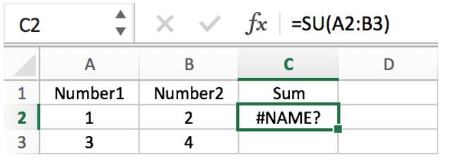
Note: You don’t need to type functions in all caps, like =ROUND, as Excel will automatically capitalize the function name for you once you press enter. If you misspell a function name, like =SUME(A1:A10) instead of =SUM(A1:A10), then Excel will return a #NAME? error.
Entering Excel functions
When you create a formula that contains a function, you can use the Insert Function dialog box to help you enter worksheet functions. Once you select a function from the Insert Function dialog Excel will launch a function wizard, which displays the name of the function, each of its arguments, a description of the function and each argument, the current result of the function, and the current result of the entire formula.
To make it easier to create and edit formulas and minimize typing and syntax errors, use Formula AutoComplete. After you type an = (equal sign) and beginning letters of a function, Excel displays a dynamic drop-down list of valid functions, arguments, and names that match those letters. You can then select one from the drop-down list and Excel will enter it for you.
Nesting Excel functions
In certain cases, you may need to use a function as one of the arguments of another function. For example, the following formula uses a nested AVERAGE function and compares the result with the value 50.
1. The AVERAGE and SUM functions are nested within the IF function.
Valid returns When a nested function is used as an argument, the nested function must return the same type of value that the argument uses. For example, if the argument returns a TRUE or FALSE value, the nested function must return a TRUE or FALSE value. If the function doesn’t, Excel displays a #VALUE! error value.
Nesting level limits A formula can contain up to seven levels of nested functions. When one function (we’ll call this Function B) is used as an argument in another function (we’ll call this Function A), Function B acts as a second-level function. For example, the AVERAGE function and the SUM function are both second-level functions if they are used as arguments of the IF function. A function nested within the nested AVERAGE function is then a third-level function, and so on.
Источник
Using the CALL and REGISTER functions
Important: Caution Incorrectly editing the registry may severely damage your operating system, requiring you to reinstall it. Microsoft cannot guarantee that problems resulting from editing the registry incorrectly can be resolved. Before editing the registry, back up any valuable data. For the most recent information about using and protecting your computer’s registry, see Microsoft Windows Help.
This article describes the formula syntax and usage of the CALL, REGISTER, and REGISTER.ID functions in Microsoft Excel.
Note: The CALL and REGISTER functions are not available in Excel for the web.
In this article
Description
The following describes the argument and return value data types used by the CALL, REGISTER, and REGISTER.ID functions. Arguments and return values differ slightly depending on your operating environment, and these differences are noted in the data type table.
Data Types
In the CALL, REGISTER, and REGISTER.ID functions, the type_text argument specifies the data type of the return value and the data types of all arguments to the DLL function or code resource. The first character of type_text specifies the data type of the return value. The remaining characters indicate the data types of all the arguments. For example, a DLL function that returns a floating-point number and takes an integer and a floating-point number as arguments would require «BIB» for the type_text argument.
The following table contains a complete list of the data type codes that Microsoft Excel recognizes, a description of each data type, how the argument or return value is passed, and a typical declaration for the data type in the C programming language.
Logical
(FALSE = 0), TRUE = 1)
IEEE 8-byte floating-point number
Null-terminated string (maximum string length = 255)
Byte-counted string (first byte contains length of string, maximum string length = 255 characters)
IEEE 8-byte floating-point number
Null-terminated string (maximum string length = 255 characters)
Reference (modify in place)
Byte-counted string (first byte contains length of string, maximum string length = 255 characters)
Reference (modify in place)
Unsigned 2-byte integer
unsigned short int
Signed 2-byte integer
Signed 4-byte integer
Logical
(FALSE = 0, TRUE = 1)
Signed 2-byte integer
Signed 4-byte integer
Three arguments are passed:
unsigned short int *
unsigned short int *
double [ ]
Microsoft Excel OPER data structure
Microsoft Excel XLOPER data structure
The C-language declarations are based on the assumption that your compiler defaults to 8-byte doubles, 2-byte short integers, and 4-byte long integers.
In the Microsoft Windows programming environment, all pointers are far pointers. For example, you must declare the D data type code as unsigned char far * in Microsoft Windows.
All functions in DLLs and code resources are called using the Pascal calling convention. Most C compilers allow you to use the Pascal calling convention by adding the Pascal keyword to the function declaration, as shown in the following example: pascal void main (rows,columns,a)
If a function uses a pass-by-reference data type for its return value, you can pass a null pointer as the return value. Microsoft Excel will interpret the null pointer as the #NUM! error value.
Additional Data Types Information
This section contains detailed information about the F, G, K, O, P, and R data types and other information about the type_text argument.
F and G Data Types
With the F and G data types, a function can modify a string buffer that is allocated by Microsoft Excel. If the return value type code is F or G, then Microsoft Excel ignores the value returned by the function. Instead, Microsoft Excel searches the list of function arguments for the first corresponding data type (F or G) and then takes the current contents of the allocated string buffer as the return value. Microsoft Excel allocates 256 bytes for the argument, so the function may return a larger string than it received.
K Data Type
The K data type uses a pointer to a variable-size FP structure. You must define this structure in the DLL or code resource as follows:
The declaration double array[1] allocates storage for only a single-element array. The number of elements in the actual array equals the number of rows multiplied by the number of columns.
O Data Type
The O data type can be used only as an argument, not as a return value. It passes three items: a pointer to the number of rows in an array, a pointer to the number of columns in an array, and a pointer to a two-dimensional array of floating-point numbers.
Instead of returning a value, a function can modify an array passed by the O data type. To do this, you can use «>O» as the type_text argument. For more information, see «Modifying in Place — Functions Declared as Void» below.
The O data type was created for direct compatibility with Fortran DLLs, which pass arguments by reference.
P Data Type
The P data type is a pointer to an OPER structure. The OPER structure contains 8 bytes of data, followed by a 2-byte identifier that specifies the type of data. With the P data type, a DLL function or code resource can take and return any Microsoft Excel data type.
The OPER structure is defined as follows:
typedef struct _oper
The type field contains one of these values.
Val field to use
String (first byte contains length of string)
Error: the error values are:
The last two values can be used only as arguments, not return values. The missing argument value (128) is passed when the caller omits an argument. The empty cell value (256) is passed when the caller passes a reference to an empty cell.
R Data Type — Calling Microsoft Excel Functions from DLLs
The R data type is a pointer to an XLOPER structure, which is an enhanced version of the OPER structure. In Microsoft Excel version 4.0 and later, you can use the R data type to write DLLs and code resources that call Microsoft Excel functions. With the XLOPER structure, a DLL function can pass sheet references and implement flow control, in addition to passing data. A complete description of the R data type and the Microsoft Excel application programming interface (API) is beyond the scope of this topic. The Microsoft Office XP Developer’s Guide contains detailed information about the R data type, the Microsoft Excel API, and many other technical aspects of Microsoft Excel.
Volatile Functions and Recalculation
Microsoft Excel usually calculates a DLL function (or a code resource) only when it is entered into a cell, when one of its precedents changes, or when the cell is calculated during a macro. On a worksheet, you can make a DLL function or code resource volatile, which means that it recalculates every time the worksheet recalculates. To make a function volatile, add an exclamation point (!) as the last character in the type_text argument.
For example, in Microsoft Excel for Windows, the following worksheet formula recalculates every time the worksheet recalculates:
Modifying in Place — Functions Declared as Void
You can use a single digit n for the return type code in type_text, where n is a number from 1 to 9. This tells Microsoft Excel to modify the variable in the location pointed to by the nth argument in type_text, instead of returning a value. This is also known as modifying in place. The nth argument must be a pass-by-reference data type (C, D, E, F, G, K, L, M, N, O, P, or R). The DLL function or code resource must also be declared with the void keyword in the C language (or the procedure keyword in the Pascal language).
For example, a DLL function that takes a null-terminated string and two pointers to integers as arguments can modify the string in place. Use «1FMM» as the type_text argument, and declare the function as void.
Versions prior to Microsoft Excel 4.0 used the > character to modify the first argument in place; there was no way to modify any argument other than the first. The > character is equivalent to n = 1 in Microsoft Excel version 4.0 and later.
Источник
Excel Function Arguments
Excel 2019 All-in-One For Dummies

Most of the functions found in Excel require some input or information in order to calculate correctly. For example, to use the AVERAGE function, you need to give it a range of numbers to average.
Any input you give to a function is called an argument.
The basic construct of a function is:
To use a function, you enter its name, open parenthesis, the needed arguments, and then the close parenthesis. The number of arguments needed varies from function to function.
Using functions with no arguments
Some functions, such as the NOW() function, don’t require any arguments. To get the current date and time, you can simply enter a formula like this:
Note that even though no arguments are required, you still need to include the open and close parentheses.
Using functions with one or more required arguments
Some functions require one or more arguments. The LARGE function, for instance, returns the nth largest number in a range of cells. This function requires two arguments: a cell reference to a range of numeric values and a rank number. To get the third largest value in range A1 through A100, you can enter:
Note that each argument is separated by a comma. This is true regardless of how many arguments you enter. Each argument must be separated by a comma.
Using functions with both required and optional arguments
Many Excel functions, such as the NETWORKDAYS function, allow for optional arguments in addition to the required arguments. The NETWORKDAYS function returns the number of workdays (days excluding weekends) between a given start date and end data.
To use the NETWORKDAYS function, you need to provide, at minimum, the start and end dates. These are the required arguments.
The following formula gives you the answer 260, meaning that there are 260 workdays between January 1, 2014, and December 31, 2014:
The NETWORKDAYS function also allows for an optional argument that lets you pass a range containing a list of holiday dates. The function treats each date in the optional range as a nonworkday, effectively returning a different result (255 workdays between January 1, 2014, and December 31, 2014, taking into account holiday dates).
Don’t be too concerned with completely understanding the NETWORKDAYS function. The take-away here is that when a function has required and optional arguments, you can elect to use the function with just the required arguments, or you can take advantage of the function’s additional utility by providing the optional arguments.
Finding out which arguments are needed for a given function
An easy way to discover the arguments needed for a given function is to begin typing that function into a cell. Click a cell, enter the equal sign, enter the function name, and then enter an open parenthesis.
Recognizing that you are entering a function, Excel activates a tooltip that shows you all the arguments for the function. Any argument that is shown in brackets ([ ]) is an optional argument. All others shown without the brackets are required arguments.
Источник
![]()
Function Arguments in Excel

Arguments in Excel Functions are input values to an Excel Function. Most of the Excel Functions will take one or more arguments, will be used in the function programs as input data and return the outputs. For example, Trim Function will take a string as input (argument) and returned the output by removing the extra spaces from the string.
Data Types of Parameters
Optional Arguments
Required Arguments
Functions with no Arguments
Functions with One Arguments
Functions with Multiple Arguments
Arguments Separator
what is an argument in excel
how to separate arguments in excel
what is an optional argument in excel
what are the values inside the parentheses of a function known as in excel
function arguments excel calculator
what does the excel argument nper refer to?
what symbol is placed between arguments in a formula
the arguments inside the parentheses of a function provide what purpose
Share This Story, Choose Your Platform!
Leave A Comment Cancel reply
Save my name, email, and website in this browser for the next time I comment.
© Copyright 2012 – 2020 | Excelx.com | All Rights Reserved
Page load link
Arguments are the values that functions use to perform calculations. In spreadsheet programs such as Excel and Google Sheets, functions are just built-in formulas that carry out set calculations and most of these functions require data to be entered, either by the user or another source, in order to return a result.
Function Syntax
A function’s syntax refers to the layout of the function and includes the function’s name, parenthesis, comma separators, and its arguments.
The arguments are always surrounded by parentheses and individual arguments are separated by commas.
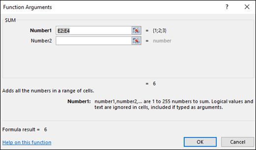
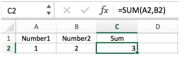
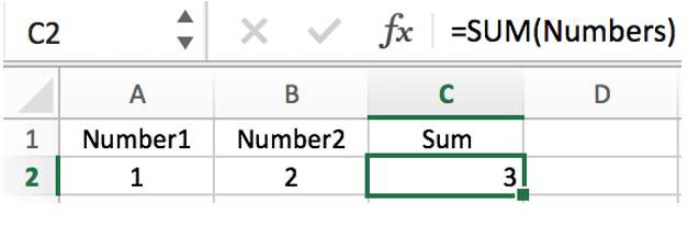
A simple example, shown in the image above, is the SUM function, which can be used to sum or total long columns or rows of numbers. The syntax for this function is:
SUM (Number1, Number2, ... Number255)
The arguments for this function are:
Number1, Number2, ... Number255
Number of Arguments
The number of arguments that a function requires varies with the function. The SUM function can have up to 255 arguments, but only one is required — the Number1 argument. The remainder are optional.
The OFFSET function, meanwhile, has three required arguments and two optional ones.
Other functions, such as the NOW and TODAY functions, have no arguments but draw their data — the serial number or date — from the computer’s system clock. Even though no arguments are required by these functions, the parentheses, which are part of the function’s syntax, must still be included when entering the function.
Types of Data in Arguments
Like the number of arguments, the types of data that can be entered for an argument will vary depending upon the function.
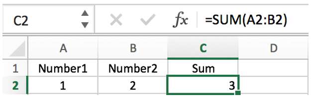
In the case of the SUM function, as shown in the image above, the arguments must contain number data, but this data can be:
- the actual data being summed — the Number1 argument in the image above
- an individual cell reference to the location of the number data in the worksheet — the Number2 argument
- an array or range of cell references — the Number3 argument
Other types of data that can be used for arguments include:
- text data
- Boolean values
- error values
- other functions
Nesting Functions
It is common for one function to be entered as the argument for another function. This operation is known as nesting functions and it is done to extend the capabilities of the program in carrying out complex calculations.
For example, it is not uncommon for IF functions to be nested one inside the other as shown below.
=IF(A1 > 50,IF(A2 < 100, A1 * 10,A1 * 25)
In this example, the second or nested IF function is used as the Value_if_true argument of the first IF function and is used to test for a second condition, if the data in cell A2 is less than 100.
Since Excel 2007, 64 levels of nesting are permitted in formulas. Prior to that, only seven levels of nesting were supported.
Finding a Function’s Arguments
Two ways of finding the argument requirements for individual functions are:
- Open the function’s dialog box in Excel
- Tooltip windows in Excel and Google Sheets
Excel Function Dialog Boxes
The vast majority of functions in Excel have a dialog box, as shown for the SUM function in the image above, that lists the required and optional arguments for the function.
Opening a function’s dialog box can be done by:
- finding and clicking on a function’s name under the Formula tab of the ribbon;
- clicking on the Insert Function option located next to the formula bar, as indicated in the image above.
Tooltips: Typing a Function’s Name
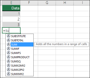
Another way to find out a function’s arguments in Excel and in Google Sheets is to:
-
Select a cell.
-
Enter the equal sign to notify the program that a formula is being entered.
-
Enter the function’s name.
As you type, the names of all functions starting with that letter appear in a tooltip below the active cell.
-
Enter an open parenthesis — the specified function and its arguments are listed in the tooltip.
In Excel, the tooltip window surrounds optional arguments with square brackets ([ ]). All others listed arguments are required.
In Google Sheets, the tooltip window does not differentiate between required and optional arguments. Instead, it includes an example as well as a summary of the function’s use and a description of each argument.
Thanks for letting us know!
Get the Latest Tech News Delivered Every Day
Subscribe
Home / What is a Function in Excel
Home / What is a Function in Excel
What is a Function in Excel
In Excel, a function is a predefined formula that performs a specific calculation by using values a user input as arguments. Every Excel function has a specific purpose, in simple words, it calculates a specific value. Each function has its arguments (the value one needs to input) to get the result value in the cell.
Components
Each function has two major components. In short, each function (except a few) is made up of two following things:
- Function Name
- Arguments
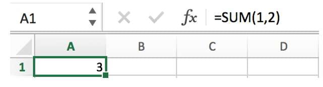
Let me show you an example. Let’s take a look at the below function which we have inserted in the cell A1.
Now if you look at the formula bar you can understand the structure of the function by splitting it into two parts i.e. name and arguments.
Function Arguments
As I have already mentioned that in a function you need to specify input values to get the desired result. An argument is that value which you need to specify. If you look at the syntax of a function you can see there in each function there is set arguments to specify.
Below are the types of arguments:
- Required: A required argument is compulsory for a user to specify and without which a function can’t calculate its result.
- Optional: If you skip specifying these arguments it will not stop a function to calculate its result value.
- No Arguments: There are few functions (like NOW) where you don’t need to specify any argument.
How to INSERT a Function in Excel
The easiest way to insert a function in a cell in Excel is to type the name of the function you want to insert starting with equals to sign.
Let’s say you want to insert the SUM function:
- First of all, you need to type = and the then type SUM.
- After that, enter the opening parentheses.
- Specify the arguments (refer to a cell or you can directly enter values into the function).
- In the end, type closing parentheses and hit enter.
Major Types
Below are the major types:
- Text Functions: If you deal with data where you have text, then below are some of the functions which you need to learn to work efficiently.
- Date Functions: Dates are one of the major ingredients of data that you use every day, and helps you to analyze your data in a better way.
- Time Functions: Just like dates, time is could also be there in data and you can use time functions to deal with data where you have time values.
- Logical Functions: Logical functions can help you create some of the most helpful formula in your spreadsheet.
- Maths Functions: Excel is all about calculations and analysis, and mathematical functions and you can use these functions to get better in calculations and analysis.
- Statistical Functions: One of the best things about Excel is there are a bunch of statistical functions there that you can use to analyze data easily.
- Lookup Functions: In Excel, there some specific functions which can help you to look up a value or specific information about a cell or a range of cells.
- Information Function: These some specific functions which you can use to get information about the values you supplied.
- Financial Functions: These functions can help you calculate some of the common but important financial calculations in an easy way.
About the Author

Puneet is using Excel since his college days. He helped thousands of people to understand the power of the spreadsheets and learn Microsoft Excel. You can find him online, tweeting about Excel, on a running track, or sometimes hiking up a mountain.
Still cannot understand the functions and formulas in Excel or google sheets and trouble? The most basic excel or google sheets function parameters introduction, newcomers must see!
Table of Contents
- ABSTRACT
- – Arguments
- – Constants
- – Cell Reference & Range Reference
- Cell Reference
- Range Reference
- Relative Reference:
- Absolute Reference:
- Mixed Reference:
- – Array
- – Logical Values
- – Logical Operators
- AND
- NOT
- OR
- IF
- – Error Values
- Error: #NAME?
- Error: #N/A
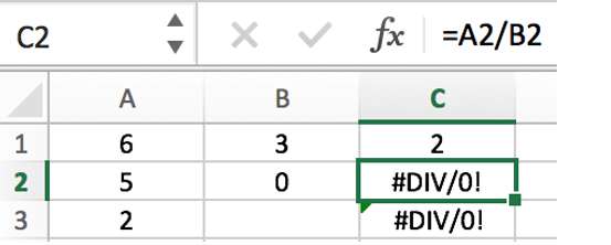
- Error: #DIV/0!
- Error: #NUM!
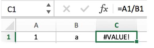
- Error: #VALUE!
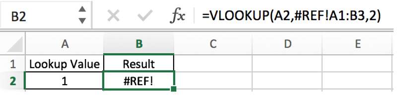
- Error: #REF!
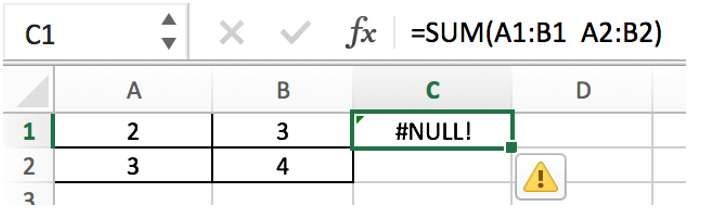
- Error: #NULL!
- Resolution
- – Nested Functions
ABSTRACT
Our website introduces many basic uses of functions in Excel or google sheets as well as common examples from everyday life and work. We have also uploaded many articles on how to use functions to create formulas to solve common problems.
We found that, in fact, many people do not know much about Excel or google sheets functions, or a half-understanding, by reading our articles may solve the current problem, but they do not know how to use Excel or google sheets functions to create formulas when solving the problem, with what function? Which similar function to use? How to nest the formula? What is the input value? Why does it return an error?
We will have the above problems because we usually only think about how to quickly apply these functions as well as formulas to solve problems in a timely manner, and copy the formula directly to use it without thinking about how the formula works.
We will face a lot of problems, so before we learn Excel or google sheets functions and formulas, we must learn some basic concepts about functions and formulas, or a few basic elements that make up a function/formula. Then after understanding these basic concepts, you will really see how a formula is made up and what role each part plays in the formula.
– Arguments
Referring to the syntax structure of the function, each item in the function brackets is called an argument to the function. These arguments can be constants, cell reference, range reference, arrays, nested functions, etc. Next, we will introduce them according to different categories of arguments.
In the example below, number 1 and 2 are arguments to SUM function.
– Constants
Constant is an immutable value or data item. A constant can be a specified value, array, or character/string. In a normal Excel or google sheets formula, in addition to the value itself, you can also enter a cell reference or range reference that contains the value(s).
Note: Neither the formula nor the result calculated by the formula is a constant, because whenever the argument of the formula changes, it will affect the formula calculation and change the result.
In the example below, arguments 1 and 2 are entered manually, they are constants.
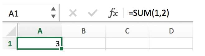
– Cell Reference & Range Reference
Cell reference and cell range reference are the most common arguments in Excel or google sheets functions. The purpose of the reference is to define the cell or range in the worksheet and specify the location of the data used by the formula or function, so that the function can easily use the data in various parts of the worksheet.
The values in cell references and range references can be static values, but they can also be dynamic values. The actual return value according to the change in the value of cell reference or range reference.
Cell Reference
In the example below, A2 and B2 are cell references. Number “1” is saved in cell reference A2, “2” is saved in cell B2. When selecting A2 in a function, that means number “1” in A2 is referenced.
A cell reference is delivered to function as its argument.
Range Reference
The entire selected multiple cells can be seen a range reference. In Excel or google sheets, for the common used lookup function VLOOKUP, its lookup range argument is usually entered with a range reference.
In the example below, A2:B2 is a range reference, it is one argument to SUM function not two arguments. This range reference contains an array actually. We will introduce array in the following paragraph.
When entering or typing function’s arguments, we can click on a single cell, or drag and drop to select multiple cells, in this way we can directly enter a cell reference or range reference.
We can also pre-define a name for a range reference in advance, in this way, we can enter this name directly as function’s argument when applying a function.
STEP 1: Name a range reference:
Formulas->Define Name, enter “Numbers” for selected range:
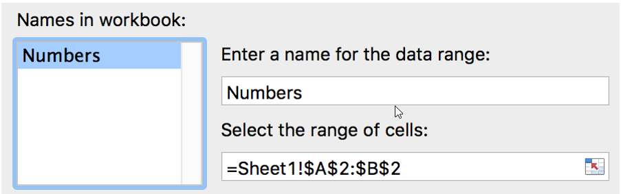
OR
Select A1:B2->Enter “Numbers” in Name Box:
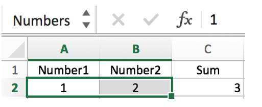
STEP 2: Entering “Numbers” as argument.
As functions or formulas are often copied directly to other cells through drag-and-drop operations, usually, the reference will change automatically according to the cell location where the formula is located.
If you do not want to change the reference, we must add a dollar sign in front of the row or column index. For these two cases, we divided the reference into relative reference and absolute reference.
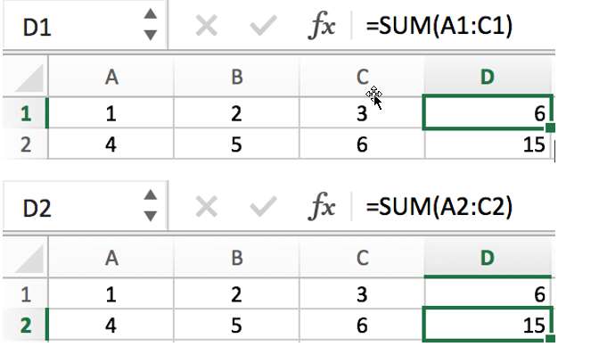
Relative Reference:
When dragging down the formula, A1:C1 is automatically updated to A2:C2.
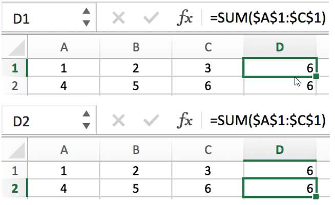
Absolute Reference:
When dragging down the formula, $A$1:$C$1 is not changed. Because we add $ before row and column indexes, so range reference is locked.
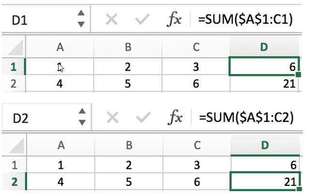
Mixed Reference:
When dragging down the formula, for range reference $A$1:C1, $A$1 is locked, but C1 is updated from C1 to C2 as formula is copied down to D2.
– Array
Array, equivalent to our mathematical matrix, a matrix contains multiple elements, elements and different combinations of elements constitute a matrix of different dimensions.
In EXCLE workbook, the selected range can be expressed as an array, expressed as an N row * M column area, N and M are not 0.
The array formula is relative to the ordinary function formula; it has two characteristics.
1) Elements of the array are referenced by brackets {} and separated by commas or semicolons.
2) After entering an array formula, you must press Ctrl+Shift+Enter to load the result.
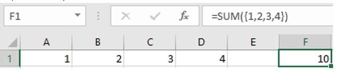
Example 1:
F1=SUM(A1:D1); A1:D1={1,2,3,4}; If all elements in on array are in one row, values are separated by comma.
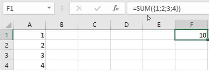
Example 2:
F1=SUM(A1:A4); A1:A4={1;2;3;4}; If all elements in on array are in one column, values are separated by semicolon.
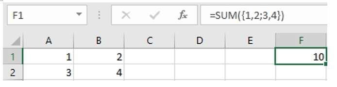
Example 3:
F1=SUM(A1:B2); A1:B2={1,2;3,4}; The array is a multidimensional array.
– Logical Values
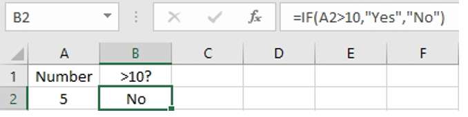
There are TRUE and FALSE two logical values. In Excel or google sheets, IF function is a logical test function that returns the corresponding branch value based on the two logical values TRUE and FALSE.
Example:
If logical test value is TRUE, IF function returns “Yes” else returns “No”.
– Logical Operators
AND
Syntax: AND(logical1, logical2, …).
Description: Returns TRUE if all arguments are true; and If AND function detects an argument with a value of false, it returns false
Example:
If both conditions “N>3” and “M>5” are true, result is TRUE.
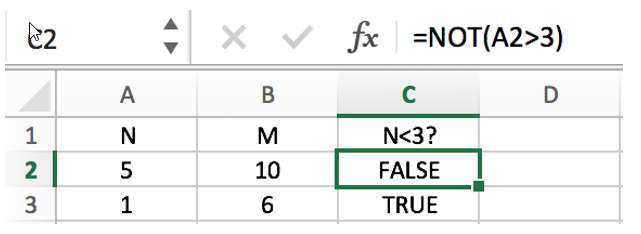
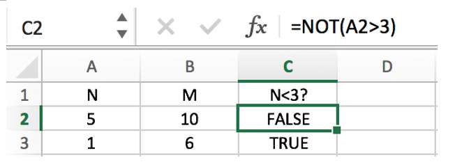
NOT
Syntax: NOT(logical)
Description: Find the opposite of a logical value or a logical expression. If you want to get the opposite of a logical value, you should use the NOT function.
Example:
Normally we can use IF function to create a logical test like =IF(A2>3,”TRUE”,”FALSE”) to return TRUE or FALSE result; Actually you can make it easier, you can also use “=NOT(A2>3)” to return the result of logical test “N<3”.
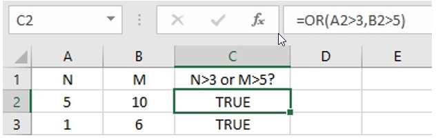
OR
Syntax: OR(logical1, logical2, …)
Description: Returns TRUE when any of the logical values is true.
Example:
If one of the conditions “N>3” and “M>5” is true, result is TRUE.
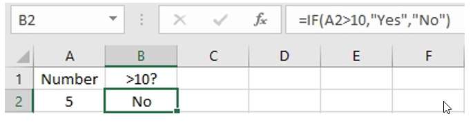
IF
The IF function is used to make logical judgments
Syntax: IF(logical_test, value_if_true, value_if_false)
Description: IF function performs a logical test which can return different results depending on the TRUE or FALSE of the logical expression.
Example:
Set “Yes” to logical test value of TRUE; Set “No” to logical test value of FALSE.
– Error Values
Sometimes we don’t get the value we want after pressing the Enter key, and formula returns error value instead. These values usually consist of “#error!”.
When we find that an error is returned, we need to understand the meaning of these errors, they can help us to know what the cause of the error is and how to solve the error.
Below is a list of common error values and solutions in Excel or google sheets function applications.
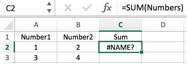
Error: #NAME?
Explanation: The function was entered incorrectly with unrecognized text. For example, the function name is spelled incorrectly, the quoted text is not quoted, and so on.
Solution: Check for spelling errors, quotation marks and brackets
Example1: Function name “SUM” is spelled incorrectly
Example2: Reference “Numbers” is missing
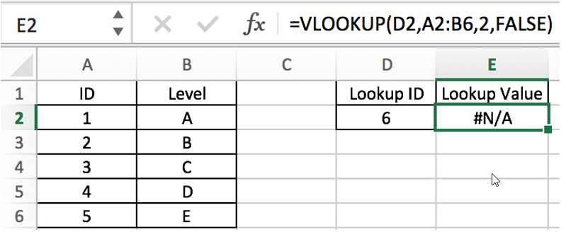
Error: #N/A
Explanation: The lookup range cannot be found when using some lookup functions in Excel workbook (for example, the VLOOKUP function cannot find the input lookup range, or the lookup value cannot be found in the first column of the lookup range).
Solution: Check if the lookup range has been entered incorrectly; make sure the lookup value is in the first column of the lookup range.
Example 1: Lookup ID doesn’t exist in lookup table A2:B6.
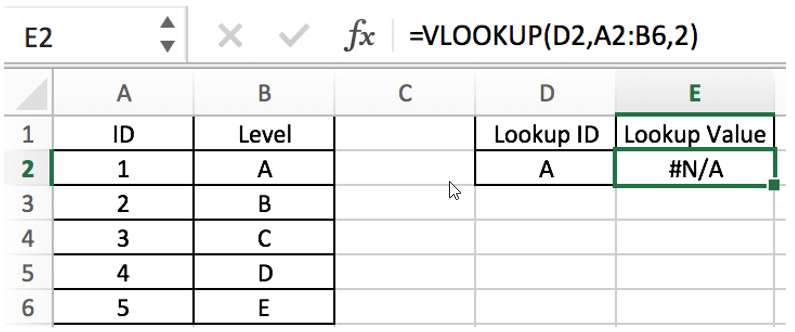
Example 2: Lookup value is incorrect; A is not listed in the first column of lookup table A2:B6.
Error: #DIV/0!
Description: Function or formula has a divisor equal to 0 or the divisor cell is empty.
Solution: Change the divisor to a non-zero value.
Example:
Error: #NUM!
Explanation: A non-numeric value has been entered in the numeric argument or is out of Excel’s calculation range.
Solution: Check the argument type and enter a valid type.
Error: #VALUE!
Explanation: Incorrect argument type entered, e.g., a number needs to be entered but text is entered, a value needs to be entered but multiple values are entered, etc. If it is an array formula, forget to press Control+Shift+Enter.
Solution: Check the argument type of the function and enter the correct type.
Example:
Divisor is “a”.
Error: #REF!
Explanation: Cell reference or range reference is invalid. For example, clear value in the cell reference which is used by the formula, then formula reports this error code.
Solution: make sure reference is correct; check if the cell reference or range reference is empty, and if it is, re-enter values into values.
Example:
Lookup table exists in sheet2, but sheet2 is deleted.
Error: #NULL!
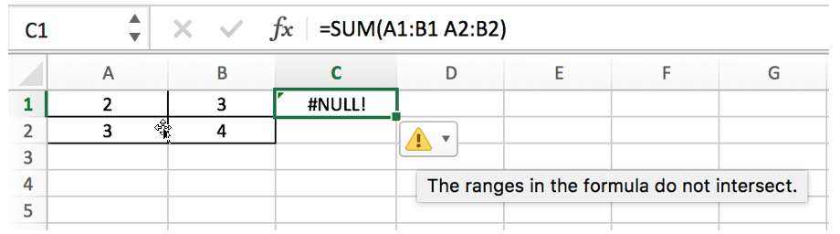
Explanation: When multiple ranges are entered, the separator is incorrect; the intersection of multiple ranges is empty.
Solution: Change the separator; make the ranges intersect.
Example:
Separator is incorrect. It should be =SUM(A1:B1,A2:B2).
Resolution
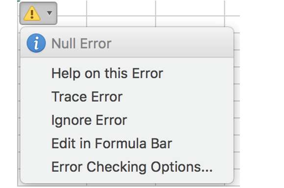
We can move mouse over the warning icon to show the floating indication message.
You can also click the icon to do the following operations.
– Nested Functions
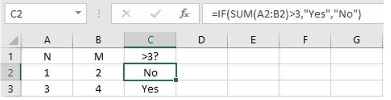
In addition to the arguments listed above, functions can also be used as arguments to a function, this is called nested function. The value of this internal function will be delivered to the external function as an argument value.
Example:
SUM(A2:B2)>3 is an argument (logical test) to IF function.
This article introduces some basic concepts in Excel or google sheets function applications, which are the most basis information for new learners. You can bookmark this article so that you can refer to it when learning functions or building formulas.
15 Most Common Excel Functions You Must Know + How to Use Them
Microsoft Excel is one of the most well-known computer applications. It has changed the way people and companies work with data.
Thus, learning Excel can help with both your career and your personal needs.
Excel runs using functions and there are roughly 500 of them! These range from basic arithmetic to complex statistics.

If you’re a new Excel user, this sheer quantity can be quite daunting.
So we are here to help you! 🤝
We have rounded up 15 of the most common and useful Excel functions that you need to learn. We also prepared a practice workbook for you to follow along with the examples. Download it here.
Let’s get started!
What are Excel functions?
Excel is used to calculate and manipulate numbers and text. To do this, you use formulas!
Formulas are expressions that tell Excel what you want to do with the data. They begin with the equal symbol (=) followed by a combination of operators and functions.
What are operators?
These are symbols that specify the type of calculation you want to perform on the elements of a formula.
For example, to add two numbers, you can type “=1+1” into a cell. Once you hit Enter, Excel will run the formula and return the result which is 2.
Here are some examples of common operators:

Excel automatically treats cell contents that start with (=) as formulas. This also applies when you begin a cell with the plus (+) or minus (-) symbols.
You can bypass this by adding a leading apostrophe (‘). This is how you can show formulas as text like in the table above.
Order of operation and using parentheses in Excel formulas
Generally, Excel follows PEMDAS when calculating formulas. PEMDAS means parentheses first, then exponents, then multiplication and division, then addition and subtraction.

What are functions?
These are predefined processes in Excel. Each function in Excel has a unique name and specific input(s). The function takes these inputs and performs the corresponding calculation.
The inputs or arguments of an Excel function are always enclosed in parentheses.
For example, this is the syntax for the MAX function:
=MAX(number1, [number2], …)
The list of numbers where you want to find the maximum value is placed inside the parentheses.

Using a cell or a range as input
As you learn more about Excel, you’ll find that Excel formulas rarely consist of individual numbers only like in the formula “=1+1”.

Thus, referencing cells is important in Excel and you can learn more by clicking here.
Alright! You’ve just learned how a function in Excel works.
Let’s dive right into the list! 🤿
We will start with basic Excel functions and then move on to more advanced functions.
Basic Math Functions (Beginner Level ★☆☆)
1. SUM
This is the first function in Excel that most new users need. As the name implies, the SUM function adds up all the values in a specified group of cells or range.
Syntax: =SUM(number1, [number2], …)
Try it out in the practice workbook.

If you want to get the total quiz score for each student, you can use the SUM function. In this case, the input range will be all four quiz scores for each student.
1. Type this formula into cell F2:
=SUM(B2:E2)
You can also type “=SUM(B2,C2,D2,E2)” but “=SUM(B2:E2)” is much simpler.

2. Press Enter. Excel then evaluates the formula and the cell returns the number for the total which is 360.
3. Copy this for the rest of the students or drag down the fill handle.

Notice that the SUM function ignores the cells containing text. (“X” meaning the student was unable to take the quiz)
Most of the basic math functions in Excel ignore non-numeric values such as text, date, and time.
2. COUNT
Next up is the COUNT function. It returns the number of cells containing numeric values within the input range.
Syntax: =COUNT(value1, [value2], …)
1. To get the number of quizzes taken by each student, use this formula in cell G2:
=COUNT(B2:E2)
2. Hit Enter and fill in the rows below.

If you would like to include non-numeric values in the count, you can use the COUNTA function. To count the number of blank cells, you can use the COUNTBLANK function.
Learn more about the COUNT function and its variants here.
3. AVERAGE
The average of a list of numbers is just the total divided by how many numbers there are in that list.
This is easy enough to calculate the quiz scores. You already have the SUM and the COUNT of quizzes for each student.
But, it gets even easier using the AVERAGE function in Excel.
Syntax: =AVERAGE (value1, [value2], …)
1. Type this into cell H2:
=AVERAGE(B2:E2)
2. Hit Enter and fill in the rows below.


Logical Functions (Intermediate Level – ★★☆)
Let’s raise the difficulty level a little bit.
A logical function in Excel allows you to make comparisons and use the results to change how a formula calculates.
4. IF
The IF function is a very popular function in Excel and it is actually quite easy to learn.
Syntax: =IF(logical_test, value_if_true, [value_if_false])
This function checks if a logical test is either TRUE or FALSE. It then returns the specified value based on the result.

Using the average score of each student, try to assign PASS or FAIL grades. Assume that the passing score for this class is 60.
1. Begin the formula in cell C2 with “=IF(“
The logical_test is to check if the average score in Column B is greater than or equal to (>=) the passing score of 60.
2. So, the formula becomes:
=IF(B2>=60,
If the comparison returns TRUE, then the formula should return the text “PASS”. Thus, the value_if_true argument should be “PASS”.
And if it returns FALSE, then the value_if_false argument should be “FAIL”.
3. Thus, the formula becomes:
=IF(B2>=60,”PASS”,”FAIL”)
4. Hit Enter and fill in the rows below.

What if you needed to assign grades according to a scale instead of just “PASS” and “FAIL”?
For that, you have to use multiple criteria or logical tests. While this is possible using nested IF functions, it can get messy very quickly. Instead, you can use the IFS function.
5. IFS function
The IFS function was introduced in Excel 2016 to replace nested IF functions.
This function works by evaluating the first logical test or criteria. It returns the corresponding value if it is TRUE. But if it is FALSE, the function proceeds to evaluate the second criteria, and so on.
📖 In other words, the IFS function outputs the value that corresponds to the first specified criteria that is true.
Syntax: =IFS(logical_test1, value_if_true1, [logical_test2], [value_if_true2],..)

1. First, the formula should check if the average score (column B) is above or equal to 90. If yes, it should return “A”.
=IFS(B2>=90,”A”,
2. If not, it should then check if the average score is greater than or equal to 80. If yes, it should return “B”. If you do this up to grade D, the formula becomes:
=IFS(B2>=90,”A”,B2>=80,”B”,B2>=70,”C”,B2>=60,”D”,
3. For the last grade “F”, put “TRUE” for the logical test.
The IFS function will only evaluate the last specified criteria if all of the previous logical values were FALSE. Thus, you can set the last criteria to always be TRUE thus making it a “catch all” statement.
The final formula is then:
=IFS(B2>=90,”A”,B2>=80,”B”,B2>=70,”C”,B2>=60,”D”,TRUE,”F”)

PRO-TIP:
You can use absolute cell references and a reference table when working with long formulas.
That way, you don’t have to revisit all of the arguments in the formula if you need to change some values.
For example, using the table and formula shown below, you can easily change the grading scale in use.
=IFS(B2>=$H$2,$F$2,B2>=$H$3,$F$3,B2>
=$H$4,$F$4,B2>=$H$5,$F$5,TRUE,$F$6)

Text Functions (Intermediate Level – ★★☆)
In this next section, you will see how Excel can also be used to manipulate text.
In the “Class List” worksheet of the practice workbook, the full name of each student is listed in Column A. Your goal is to rearrange these from “first name last name” to “last name_first name” in Column F.

To do this, you first have to extract the first name and the last name from Column A.
6. FIND
The names are separated by a space character ” “. So, you have to identify the position of the space within each text string in Column A.
The FIND function in Excel returns the number or position of a specified character or substring within another text string.
Syntax: =FIND(find_text, within_text, [start_num])
To get the position of the space ” “, type this formula:
=FIND(” “,A2)

Next, take a look at the LEN function.
7. LEN
This function returns the number of characters in a text string.
Syntax: =LEN(text)
To get the number of characters in each student’s name:
=LEN(A2)

Now you can move on to extracting the first and last name using the MID function in Excel.
8. MID
This function extracts a given number of characters from the middle of a text string.
Syntax: = MID(text, start_num, num_chars)
It is one of three text functions that are used to extract text. The other two are LEFT and RIGHT which extract text from the start and end of a text string respectively.
The first name starts at the very first character of the text string. So, you extract starting from position 1. Then the length of the first name is given by the position of the space character minus 1.
So, the formula to extract the first name or first word from a text string is:
=MID(A2,1,B2-1)
Or, you can express it directly using the FIND formula earlier.
=MID(A2,1,FIND(” “,A2)-1)

For the last name, you can extract it starting from the position of the space character plus 1. Its length is just the length of the entire text string minus the position of the space character.
=MID(A2,B2+1,C2-B2)
Or, using the FIND and LEN formulas earlier:
=MID(A2,FIND(” “,A2)+1,LEN(A2)-FIND(” “,A2))

Now you can combine the last name and the first name in the desired order using the CONCAT function.
9. CONCAT
Like IFS, CONCAT is another newly introduced function in Excel 2016. It replaced the old CONCATENATE function.
Syntax: =CONCAT(text1, [text2],…)
Combine the last name and the first name with a comma and space character “, ” in between.
=CONCAT(E2,”, “,D2)

PRO-TIP:
In the above example, you used helper columns for FIND, LEN, and MID to help build the final formula and visualize how it works.
In real-world applications, you can use a single long formula to get the results like this:
=CONCAT(MID(A2,FIND(” “,A2)+1,LEN(A2)
-FIND(” “,A2)),”, “,MID(A2,1,FIND(” “,A2)-1))

Lookup and Reference Functions (Advanced Level – ★★★)
In this final section, we will focus on functions that allow you to look for specific data points and refer to them.
Take a look at the “Schedule” worksheet.

10. COLUMN
The COLUMN function in Excel returns the column number of a given cell.
Syntax: =COLUMN([reference])
Let’s try to assign specific dates for each quiz. For example, you may want the quizzes to be held every Monday. This means that the first quiz date should be offset by 1 week or 7 days for each succeeding quiz date.
You can use the column number to multiply the 7 days offset for each week like this:
=$B$2+(COLUMN()-2)*7

Two (2) is subtracted from the column number so that the sequence starts at 1.
You can also get this result using the much simpler “=B2+7” since you are only adding a fixed number of days to each date. 🤔
But, using the COLUMN function, you can create complex patterns.
Take this pattern for example:
The quizzes are still held every Monday. But every third week, they are held on Wednesday instead.
Here is the formula for this pattern:
=$B$2+(COLUMN()-2)*7+IF(MOD(COLUMN()-1,3)=0,2,0)


The MOD function in Excel returns the remainder after a number is divided by a given divisor. It’s part of the Math & Trig group of functions.
This group includes other fun functions such as ABS which returns the absolute value of a number and ROUND which rounds a number to a specified number of digits.
Learn more about the function groups towards the end of this article!
11. ROW
Next, take a look at the ROW function. It works exactly like COLUMN but it returns the row number instead.
Syntax: =ROW([reference])
In this next example, you will assign the seating plans. You can try different seating arrangements using the ROW function.
Assume R1C1 is the seat closest to the teacher’s desk.
1. You can have the students seated one seat after another and in two columns:
=CONCAT(“R”,MOD(ROW()-6,3)*2+1,”C”,INT((ROW()-6)/3)*2+1)

2. Or they can sit in rows of 3 and columns of 2
=CONCAT(“R”,MOD(ROW()-6,2)*2+1,”C”,INT((ROW()-6)/2)*2+1)

3. You can also sit them in the farthest rows:
=CONCAT(“R”,MOD(ROW()-6,2)*4+1,”C”,INT((ROW()-6)/2)*2+1)

4. Or in the farthest columns:
=CONCAT(“R”,MOD(ROW()-6,3)*2+1,”C”,INT((ROW()-6)/3)*4+1)

Manually creating seating patterns for small sets like this one is easy. But a formula like those shown above definitely helps especially for larger sets like 50, 100, or even more.
The COLUMN and ROW functions are rarely used on their own. Like IF and IFS, you use them with other functions to change how the formula is calculated.
12. MATCH
Now, open up the “Lookup” worksheet.
In the next few examples, you will create a search feature that allows students to look up their names. They can then see their scores from past quizzes and their assigned seats for the next quizzes.
To start, you will use the MATCH function. It searches for a specified item within a given range of cells. It then returns the relative position of the first match.
Syntax: =MATCH(lookup_value, lookup_array, [match_type])
- The lookup_value is the item you want to search for. So, set this to cell B2.
- The lookup_array is the range or table array where you want to search. Use F2:F7 from the “Class List” worksheet.
- For the match_type, set this to zero so that the function searches for an exact match. (Learn more about MATCH and the different match types in this article)
The formula then becomes:
=MATCH(B2,’Class List’!F2:F7,0)

However, it only works correctly if the name is entered exactly as it is written in Column F of the Class List.
To fix this, you can use the asterisk “*” wildcard character so that searching for either first or last name works.
You can also enclose the formula in an IFNA function. This way, if the formula cannot find the given name in the table, it will return a phrase like “No result found”.


13. INDEX
The INDEX function retrieves a value from a given table array based on the provided row and column numbers.
Syntax: =INDEX (array, row_num, [col_num])
Similar to the MATCH example, you need to specify where the range or array lookup is.

For row_num, you can use the earlier MATCH result at Cell B5. Then for col_num, use 1 for the First Name:
=INDEX(‘Class List’!D2:E7,B5,1)

And set col_num to 2 for the Last Name.
=INDEX(‘Class List’!D2:E7,B5,2)

Just like that, you have a working search 🔍 formula!
This is just a small example of the countless possibilities using the INDEX and MATCH combination. Click here for more examples!
14. VLOOKUP
The VLOOKUP function in Excel works similarly to the INDEX and MATCH combination. It is faster to set up but it is less versatile. VLOOKUP also only works if your lookup array is at the leftmost of the reference table.
Syntax: =VLOOKUP (lookup_value, table_array, col_index_num, [range_lookup])
This time, you will use the First Name result (cell B6) as the lookup_value. Use this and VLOOKUP to retrieve the given student’s scores from the “Quiz Scores” worksheet.
=VLOOKUP($B$6,’Quiz Scores’!$A$2:$E$7,COLUMN(),FALSE)

For the seat assignment, use the Last Name result followed by the asterisk wild character.
=VLOOKUP($B$7&”*”,Schedule!$A$6:$E$11,COLUMN(),FALSE)

15. INDIRECT
The last function that you will be learning about today is also one of the most powerful in Excel.
INDIRECT allows you to specify cell references using text strings.
SYNTAX: =INDIRECT(ref_text, [a1])
For example, instead of typing “=A1”, you can type “=INDIRECT(“A”&1). This means you can dynamically change references.
Let’s take the INDEX & MATCH formula you used to retrieve the Last Name. You can get the same result using this formula:
=INDIRECT(“‘Class List’!”&”E”&(B5+1))

The INDIRECT function opens up so many possibilities with dynamic references in Excel. I highly this article for an in-depth tutorial on INDIRECT.
That’s it – Now what?
As you have just learned, Excel offers so many different functions to choose from. Luckily, Excel has brought them all together in the Formulas tab.

You can look for an Excel function using search keywords or you can also select from the categorical dropdowns.
For example, click on the Financial group to find functions that can help you calculate items like net present value, future value, cumulative interest paid, cumulative principal paid, etc.

You can also click on More Functions which opens up even more possibilities for advanced Excel formulas.
For example, the Statistical group is useful if you need to calculate a statistical value. This includes functions for maximum value, minimum value, forecast value, gamma function value, etc. You can insert a cumulative distribution function and other useful tools for data analysis.

Learn how to use these formulas and more by signing up for my free online Excel course.
We will help you make the most out of your Excel experience! 📈
Other relevant resources
If you enjoyed this article, you can visit my YouTube channel for more in-depth tutorials and other fun stuff!
Did you know that the Flash Fill feature can help speed up your work by automatically filling a repetitive pattern Excel detects from your data? Learn more here.
Thanks for reading! 😄
Kasper Langmann2023-02-23T11:47:15+00:00
Page load link