
Formulas are the life and blood of Excel spreadsheets. And in most cases, you don’t need the formula in just one cell or a couple of cells.
In most cases, you would need to apply the formula to an entire column (or a large range of cells in a column).
And Excel gives you multiple different ways to do this with a few clicks (or a keyboard shortcut).
Let’s have a look at these methods.
By Double-Clicking on the AutoFill Handle
One of the easiest ways to apply a formula to an entire column is by using this simple mouse double-click trick.
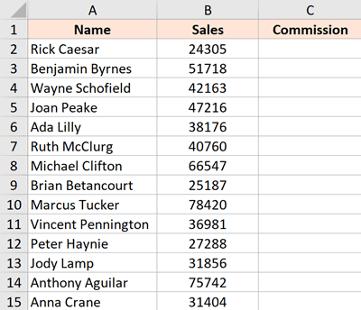
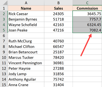
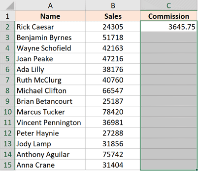
Suppose you have the dataset as shown below, where want to calculate the commission for each sales rep in Column C (where the commission would be 15% of the sale value in column B).
The formula for this would be:
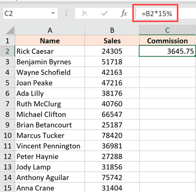
=B2*15%
Below is the way to apply this formula to the entire column C:
- In cell A2, enter the formula: =B2*15%

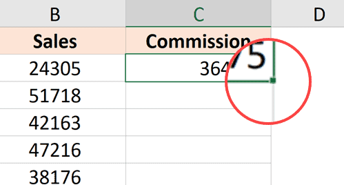
- With the cell selected, you will see a small green square at the bottom-right part of the selection.

- Place the cursor over the small green square. You will notice that the cursor changes to a plus sign (this is called the autofill handle)

- Double click the left mouse key

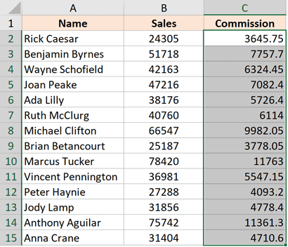
The above steps would automatically fill the entire column till the cell where you have the data in the adjacent column. In our example, the formula would be applied till cell C15
For this to work, there shouldn’t be data in the adjacent column and there should not be any blank cells in it. If, for example, there is a blank cell in column B (say cell B6), then this auto-fill double click would only apply the formula till cell C5
When you use the autofill handle to apply the formula to the entire column, it’s equivalent to copy-pasting the formula manually. This means that the cell reference in the formula would change accordingly.
For example, if it’s an absolute reference, it would remain as is while the formula is applied to the column, add if it’s a relative reference, then it would change as the formula is applied to the cells below.
By Dragging the AutoFill Handle
One issue with the above double click method is that it would stop as soon as it encountered a blank cell in the adjacent columns.
If you have a small data set, you can also manually drag the fill handle to apply the formula in the column.
Below are the steps to do this:
- In cell A2, enter the formula: =B2*15%
- With the cell selected, you will see a small green square at the bottom-right part of the selection
- Place the cursor over the small green square. You will notice that the cursor changes to a plus sign
- Hold the left mouse key and drag it to the cell where you want the formula to be applied
- Leave the mouse key when done
Using the Fill Down Option (it’s in the ribbon)
Another way to apply a formula to the entire column is by using the fill down option in the ribbon.
For this method to work, you first need to select the cells in the column where you want to have the formula.
Below are the steps to use the fill down method:
- In cell A2, enter the formula: =B2*15%
- Select all the cells in which you want to apply the formula (including cell C2)

- Click the Home tab

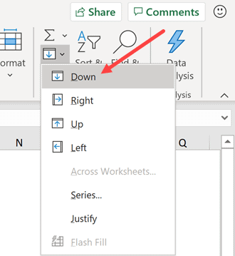
- In the editing group, click on the Fill icon

- Click on ‘Fill down’

The above steps would take the formula from cell C2 and fill it in all the selected cells
Adding the Fill Down in the Quick Access Toolbar
If you need to use the fill down option often, you can add that to the Quick Access Toolbar, so that you can use it with a single click (and it’s always visible on the screen).
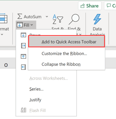
T0 add it to the Quick Access Toolbar (QAT), go to the ‘Fill Down’ option, right-click on it, and then click on ‘Add to the Quick Access Toolbar’
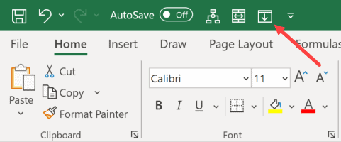
Now, you will see the ‘Fill Down’ icon appear in the QAT.
Using Keyboard Shortcut
If you prefer using the keyboard shortcuts, you can also use the below shortcut to achieve the fill down functionality:
CONTROL + D (hold the control key and then press the D key)
Below are the steps to use the keyboard shortcut to fill-down the formula:
- In cell A2, enter the formula: =B2*15%
- Select all the cells in which you want to apply the formula (including cell C2)
- Hold the Control key and then press the D key
Using Array Formula
If you’re using Microsoft 365 and have access to dynamic arrays, you can also use the array formula method to apply a formula to the entire column.
Suppose you have a data set as shown below and you want to calculate the Commission in column C.
Below is the formula that you can use:
=B2:B15*15%
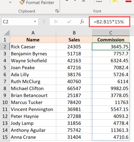
This is an Array formula that would return 14 values in the cell (one each for B2:B15). But since we have dynamic arrays, the result would not be restricted to the single-cell and would spill over to fill the entire column.
Note that you cannot use this formula in every scenario. In this case, because our formula uses the input value from an adjacent column and as the same length of the column in which we want the result (i.e., 14 cells), it works fine here.
But if this is not the case, this may not be the best way to copy a formula to the entire column
By Copy-Pasting the Cell
Another quick and well-known method of applying a formula to the entire column (or selected cells in the entire column) is to simply copy the cell that has the formula and paste it over those cells in the column where you need that formula.
Below are the steps to do this:
- In cell A2, enter the formula: =B2*15%
- Copy the cell (use the keyboard shortcut Control + C in Windows or Command + C in Mac)
- Select all the cells where you want to apply the same formula (excluding cell C2)
- Paste the copied cell (Control + V in Windows and Command + V in Mac)
One difference between this copy-paste method and all the methods convert below above this is that with this method you can choose to only paste the formula (and not paste any of the formattings).
For example, if cell C2 has a blue cell color in it, all the methods covered so far (except the array formula method) would not only copy and paste the formula to the entire column but also paste the formatting (such as the cell color, font size, bold/italics)
If you want to only apply the formula and not the formatting, use the steps below:
- In cell A2, enter the formula: =B2*15%
- Copy the cell (use the keyboard shortcut Control + C in Windows or Command + C in Mac)
- Select all the cells where you want to apply the same formula
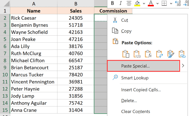
- Right-click on the Selection
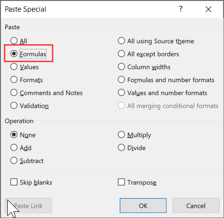
- In the options that appear, click on ‘Paste Special’

- In the ‘Paste Special’ dialog box, click on the Formulas option

- Click OK
The above steps would make sure that only the formula is copied to the selected cells (and none of the formattings comes over with it).
So these are some of the quick and easy methods that you can use to apply a formula to the entire column in Excel.
I hope you found this tutorial useful!
Other Excel tutorials you may also like:
- 5 Ways to Insert New Columns in Excel (including Shortcut & VBA)
- How to Sum a Column in Excel
- How to Compare Two Columns in Excel (for matches & differences)
- Lookup and Return Values in an Entire Row/Column in Excel
- How to Copy and Paste Columns in Excel?
- Apply Conditional Formatting Based on Another Column in Excel
- How to Multiply a Column by a Number in Excel
Follow these steps to fill a formula and choose which options to apply:
-
Select the cell that has the formula you want to fill into adjacent cells.
-
Drag the fill handle
 across the cells that you want to fill.
If you don’t see the fill handle, it might be hidden. To display it again:
-
Click File > Options
-
Click Advanced.
-
Under Editing Options, check the Enable fill handle and cell drag-and-drop box.
-
-
To change how you want to fill the selection, click the small Auto Fill Options icon
that appears after you finish dragging, and choose the option that want.
For more information about copying formulas, see Copy and paste a formula to another cell or worksheet.
Fill formulas into adjacent cells
You can use the Fill command to fill a formula into an adjacent range of cells. Simply do the following:
-
Select the cell with the formula and the adjacent cells you want to fill.
-
Click Home > Fill, and choose either Down, Right, Up, or Left.
Keyboard shortcut: You can also press Ctrl+D to fill the formula down in a column, or Ctrl+R to fill the formula to the right in a row.
Turn workbook calculation on
Formulas won’t recalculate when you fill cells if automatic workbook calculation isn’t enabled.
Here’s how you can enable it:
-
Click File > Options.
-
Click Formulas.
-
Under Workbook Calculation, choose Automatic.
-
Select the cell that has the formula you want to fill into adjacent cells.
-
Drag the fill handle
down or to the right of the column you want to fill.
Keyboard shortcut: You can also press Ctrl+D to fill the formula down a cell in a column, or Ctrl+R to fill the formula to the right in a row.
If I select a cell containing a formula, I know I can drag the little box in the right-hand corner downwards to apply the formula to more cells of the column. Unfortunately, I need to do this for 300,000 rows!
Is there a shortcut, similar to CTRL+SPACE, that will apply a formula to the entire column, or to a selected part of the column?
![]()
Asclepius
55.7k17 gold badges160 silver badges141 bronze badges
asked Mar 24, 2011 at 20:37
![]()
John ShedletskyJohn Shedletsky
7,09012 gold badges36 silver badges63 bronze badges
0
Try double-clicking on the bottom right hand corner of the cell (ie on the box that you would otherwise drag).
answered Mar 24, 2011 at 20:41
![]()
16
If the formula already exists in a cell you can fill it down as follows:
- Select the cell containing the formula and press CTRL+SHIFT+DOWN to select the rest of the column (CTRL+SHIFT+END to select up to the last row where there is data)
- Fill down by pressing CTRL+D
- Use CTRL+UP to return up
On Mac, use CMD instead of CTRL.
An alternative if the formula is in the first cell of a column:
- Select the entire column by clicking the column header or selecting any cell in the column and pressing CTRL+SPACE
- Fill down by pressing CTRL+D
![]()
Asclepius
55.7k17 gold badges160 silver badges141 bronze badges
answered Jan 18, 2013 at 3:02
![]()
robinCTSrobinCTS
5,68814 gold badges29 silver badges37 bronze badges
8
Select a range of cells (the entire column in this case), type in your formula, and hold down Ctrl while you press Enter. This places the formula in all selected cells.
answered Mar 1, 2012 at 15:28
![]()
PhilPhil
1,0597 silver badges3 bronze badges
1
Excel is essentially a calculation engine. Just like a calculator, it takes questions in the form of formulas, for example, =8+4, and returns answers.
Formulas are essential to manipulating data and extracting useful information from your Excel workbooks. Formulas make Excel roar to life as it were.
Although formulas are powerful tools they need to be used in an efficient manner for maximum benefit.
Suppose you have a dataset that requires the same formula in an entire column. Laboriously entering the formula in one cell at a time wastes time and effort.
This tutorial shows you 7 time-saving techniques for applying a formula at once to an entire column in Excel.
Method #1: Double-click the Fill Handle
The following is a dataset showing the quantities of various items bought and their prices.

We want to apply a formula in column D to calculate the total cost of each line of items bought.
We will enter a formula in cell D2 and double-click the fill handle to copy the formula down the column.
Here are the steps to do this:
- Select cell D2 and type in the following formula:
=B2*C2

- Click the Enter button on the formula bar.

This enters the formula without moving the cell selector.

Notice the little green square in the bottom right corner of cell D2:

That little green square is called the Fill Handle.
Note: If you do not see the fill handle enable it by doing the following then continue with step 3:
- Click the File tab to open the Backstage window.
- Select Options in the left sidebar.
- Select Advanced in the left sidebar of the Excel Options dialog box that appears. Then select Enable Fill handle and cell drag-and-drop and click OK.

- Hover the mouse pointer over the fill handle. It changes to a plus sign:

- Double-click the left mouse button.

The formula is copied down the column and total prices for the various items are returned.
The cell references in the formula are relative and are therefore adjusted accordingly as the formula is copied down the column. You can ascertain this by clicking Show Formulas in the Formula Auditing group on the Formulas tab.


Note: If the cell references in the formula were absolute, meaning they had two dollar signs, for example, =$B$2*$C$2, the formula would be copied down the column as is.
One problem with the technique of double-clicking the fill handle is that if there are blank rows in the dataset, the formula is not copied all the way down the column but only up to the first blank cell in the column as shown below:

If your dataset has blank rows you can first delete them before double-clicking the fill handle or use the following method of dragging down the fill handle.
Also read: Formulas Not Copying Down in Excel – How to Fix!
Method #2: Drag Down the Fill Handle
The following is a dataset showing the quantities of various items bought and their prices. Row 4 of the dataset is blank.

We want to apply a formula in column D to calculate the total cost of each line of items bought.
We will enter a formula in cell D2 and drag down the fill handle to copy the formula down the column.
Below are the steps to do this:
- Select cell D2 and type in the following formula:
=B2*C2

- Press the Enter button on the formula bar to enter the formula.

- Hover the mouse pointer over the fill handle. It changes to a plus sign. Press and hold down the left mouse button and drag the fill handle down to cell D6, then release the button.

Notice the zero (0) in cell D4. You can delete it.
One drawback of this technique is that it can become cumbersome if you are working with a large dataset.
Method #3: Use Copy and Paste
The following is a dataset showing the quantities of various items bought and their prices.

We want to apply a formula in column D to calculate the total cost of each line of items bought.
We will enter a formula in cell D2, copy it, and paste it into the rest of the cells in the column.
We use the following steps:
- Select cell D2 and type in the following formula:
=B2*C2

- Click the Enter button on the formula bar to enter the formula.

- Press Ctrl + C to copy the formula in cell D2. On a Mac use Cmd + C.

Notice the marching ants border around cell D2. This indicates that the formula in the cell is copied to the clipboard and is available for pasting.
- Select range D3:D6.

- Press Ctrl + V to paste the formula in the selected range.

The formula is copied into the range and the total price of each line of the items bought is returned.
Notice that cell D2 still has the marching ants border. Press the Escape key to remove it and clear the clipboard.
Note: If the cell containing the formula has formatting that you do not want to be copied down the column, you can use the Paste Special feature as follows:
- Select and copy the cell containing the formula.
- Select the range into which you want the formula to be copied.
- Press Ctrl + Alt + V to open the Paste Special dialog box. Select the Formulas option and click OK.

Method #4: Use a Dynamic Array Formula
The following is a dataset showing the quantities of various items bought and their prices.

We want to apply a formula in column D to calculate the total cost of each line of items bought. We will enter a dynamic array formula in cell D2. We will press Enter to automatically propagate the formula in the column.
Note: Dynamic arrays are only available in Office 365 and Office 2022 or later.
We use the following steps:
- Select cell D2 and type in the following formula:
=B2:B6*C2:C6

- Press Enter or click the Enter button on the formula bar.

The formula is propagated to the rest of the cells and the total price of each line of the items bought is returned.
Important information about dynamic array formulas
Notice the blue border around range D2:D6 in our example dataset.

When we entered the dynamic array formula, the results spilled into the range. Excel visually defines a spill range with a solid blue border.
All cells in the spill range are disabled except the cell containing the original formula. This means that none of the values in the spill range except cell D2 can be edited, deleted, or moved in any way.
The spill range must be blank for dynamic arrays to work. Any non-empty cell in the path of the spill range will cause a #SPILL! error.
For example, the following dataset has a value in cell D4.

If we attempt to enter a dynamic array formula in cell D2 we get a #SPILL! error:

Delete the value in cell D4 and the formula propagates without an error:

Method #5: Use the Fill Down Command on the Home Tab
The following is a dataset showing the quantities of various items bought and their prices.

We want to apply a formula in column D to calculate the total cost of each line of items bought. We will enter a formula in cell D2 and use the Fill Down command on the Home tab to copy the formula down the column.
We use the following steps:
- Select cell D2 and type in the following formula:
=B2*C2

- Click the Enter button on the formula bar and select range D2:D6.

- Select the Down option on the Fill drop-down list in the Editing group on the Home tab.

The formula is copied down the column and the total price of each line of items bought is returned.

Method #6: Use a Keyboard Shortcut
The following is a dataset showing the quantities of various items bought and their prices.

We want to apply a formula in column D to calculate the total cost of each line of items bought. We will enter a formula in cell D2 and use the keyboard shortcut Ctrl + D to copy the formula down the column.
We proceed as follows:
- Select cell D2 and type in the following formula
=B2*C2

- Click the Enter button on the formula bar and select range D2:D6.

- Press Ctrl + D.

The formula is copied down the column and the total price of each line of items bought is returned.
Method #7: Use Excel VBA
The following is a dataset showing the quantities of various items bought and their prices.

We want to apply a formula in column D to calculate the total cost of each line of items bought. We will create and use a VBA procedure to copy the formula down the column.
We use the following steps:
- Press Alt + F11 to open the Visual Basic Editor.
- Select Module on the Insert menu.

- Type the following procedure in the module.
Sub EnterFormulaEntireColumn()
Range("D2").Formula = "=B2*C2"
Range("D2").AutoFill Range("D2:D6")
End Sub- Save the procedure and save the workbook as a Macro-Enabled Workbook.
- Place the anywhere in the procedure and press F5 to run the code.
- Press Alt + F11 to switch back to the active worksheet.

The procedure has worked and copied the formula down the column.
Note that cell references are hard-coded in the procedure and we will need to change the cell references if we want to apply the procedure to another dataset.
In this tutorial, we have looked at 7 different techniques for applying a formula to an entire column in Excel. You can use the techniques that work best for you.
Other Excel articles you may also like:
- Unhide Columns in Excel (Keyboard Shortcut)
- How to Filter Multiple Columns in Excel? 3 Easy Ways!
- Group Rows or Columns [Keyboard Shortcut]
- How to Flip Data in Excel (Columns, Rows, Tables)?
Содержание
- How to Apply Formula to Entire Column in Excel (5 Easy Ways)
- By Double-Clicking on the AutoFill Handle
- By Dragging the AutoFill Handle
- Using the Fill Down Option (it’s in the ribbon)
- Adding the Fill Down in the Quick Access Toolbar
- Using Keyboard Shortcut
- Using Array Formula
- By Copy-Pasting the Cell
- Fill a formula down into adjacent cells
- Fill formulas into adjacent cells
- Turn workbook calculation on
- Need more help?
- Shortcut to Apply a Formula to an Entire Column in Excel [closed]
- 3 Answers 3
- Use calculated columns in an Excel table
- Create a calculated column
- Need more help?
How to Apply Formula to Entire Column in Excel (5 Easy Ways)
Formulas are the life and blood of Excel spreadsheets. And in most cases, you don’t need the formula in just one cell or a couple of cells.
In most cases, you would need to apply the formula to an entire column (or a large range of cells in a column).
And Excel gives you multiple different ways to do this with a few clicks (or a keyboard shortcut).
Let’s have a look at these methods.
This Tutorial Covers:
By Double-Clicking on the AutoFill Handle
One of the easiest ways to apply a formula to an entire column is by using this simple mouse double-click trick.
Suppose you have the dataset as shown below, where want to calculate the commission for each sales rep in Column C (where the commission would be 15% of the sale value in column B).
The formula for this would be:
Below is the way to apply this formula to the entire column C:
- In cell A2, enter the formula: =B2*15%
- With the cell selected, you will see a small green square at the bottom-right part of the selection.
- Place the cursor over the small green square. You will notice that the cursor changes to a plus sign (this is called the autofill handle)
- Double click the left mouse key
The above steps would automatically fill the entire column till the cell where you have the data in the adjacent column. In our example, the formula would be applied till cell C15
![]()
When you use the autofill handle to apply the formula to the entire column, it’s equivalent to copy-pasting the formula manually. This means that the cell reference in the formula would change accordingly.
For example, if it’s an absolute reference, it would remain as is while the formula is applied to the column, add if it’s a relative reference, then it would change as the formula is applied to the cells below.
By Dragging the AutoFill Handle
One issue with the above double click method is that it would stop as soon as it encountered a blank cell in the adjacent columns.
If you have a small data set, you can also manually drag the fill handle to apply the formula in the column.
Below are the steps to do this:
- In cell A2, enter the formula: =B2*15%
- With the cell selected, you will see a small green square at the bottom-right part of the selection
- Place the cursor over the small green square. You will notice that the cursor changes to a plus sign
- Hold the left mouse key and drag it to the cell where you want the formula to be applied
- Leave the mouse key when done
Using the Fill Down Option (it’s in the ribbon)
Another way to apply a formula to the entire column is by using the fill down option in the ribbon.
For this method to work, you first need to select the cells in the column where you want to have the formula.
Below are the steps to use the fill down method:
- In cell A2, enter the formula: =B2*15%
- Select all the cells in which you want to apply the formula (including cell C2)
- Click the Home tab
- In the editing group, click on the Fill icon
- Click on ‘Fill down’
The above steps would take the formula from cell C2 and fill it in all the selected cells
Adding the Fill Down in the Quick Access Toolbar
If you need to use the fill down option often, you can add that to the Quick Access Toolbar, so that you can use it with a single click (and it’s always visible on the screen).
T0 add it to the Quick Access Toolbar (QAT), go to the ‘Fill Down’ option, right-click on it, and then click on ‘Add to the Quick Access Toolbar’
Now, you will see the ‘Fill Down’ icon appear in the QAT.
Using Keyboard Shortcut
If you prefer using the keyboard shortcuts, you can also use the below shortcut to achieve the fill down functionality:
Below are the steps to use the keyboard shortcut to fill-down the formula:
- In cell A2, enter the formula: =B2*15%
- Select all the cells in which you want to apply the formula (including cell C2)
- Hold the Control key and then press the D key
Using Array Formula
If you’re using Microsoft 365 and have access to dynamic arrays, you can also use the array formula method to apply a formula to the entire column.
Suppose you have a data set as shown below and you want to calculate the Commission in column C.
Below is the formula that you can use:
This is an Array formula that would return 14 values in the cell (one each for B2:B15). But since we have dynamic arrays, the result would not be restricted to the single-cell and would spill over to fill the entire column.
Note that you cannot use this formula in every scenario. In this case, because our formula uses the input value from an adjacent column and as the same length of the column in which we want the result (i.e., 14 cells), it works fine here.
But if this is not the case, this may not be the best way to copy a formula to the entire column
By Copy-Pasting the Cell
Another quick and well-known method of applying a formula to the entire column (or selected cells in the entire column) is to simply copy the cell that has the formula and paste it over those cells in the column where you need that formula.
Below are the steps to do this:
- In cell A2, enter the formula: =B2*15%
- Copy the cell (use the keyboard shortcut Control + C in Windows or Command + C in Mac)
- Select all the cells where you want to apply the same formula (excluding cell C2)
- Paste the copied cell (Control + V in Windows and Command + V in Mac)
One difference between this copy-paste method and all the methods convert below above this is that with this method you can choose to only paste the formula (and not paste any of the formattings).
For example, if cell C2 has a blue cell color in it, all the methods covered so far (except the array formula method) would not only copy and paste the formula to the entire column but also paste the formatting (such as the cell color, font size, bold/italics)
If you want to only apply the formula and not the formatting, use the steps below:
- In cell A2, enter the formula: =B2*15%
- Copy the cell (use the keyboard shortcut Control + C in Windows or Command + C in Mac)
- Select all the cells where you want to apply the same formula
- Right-click on the Selection
- In the options that appear, click on ‘Paste Special’
- In the ‘Paste Special’ dialog box, click on the Formulas option
- Click OK
The above steps would make sure that only the formula is copied to the selected cells (and none of the formattings comes over with it).
So these are some of the quick and easy methods that you can use to apply a formula to the entire column in Excel.
I hope you found this tutorial useful!
Other Excel tutorials you may also like:
Источник
Fill a formula down into adjacent cells
You can quickly copy formulas into adjacent cells by dragging the fill handle  . When you fill formulas down, relative references will be put in place to ensure the formulas adjust for each row—unless you include absolute or mixed references before you fill the formula down.
Follow these steps to fill a formula and choose which options to apply:
Select the cell that has the formula you want to fill into adjacent cells.
Drag the fill handle across the cells that you want to fill.
If you don’t see the fill handle, it might be hidden. To display it again:
Click File > Options
Under Editing Options, check the Enable fill handle and cell drag-and-drop box.
To change how you want to fill the selection, click the small Auto Fill Options icon  that appears after you finish dragging, and choose the option that want.
For more information about copying formulas, see Copy and paste a formula to another cell or worksheet.
Fill formulas into adjacent cells
You can use the Fill command to fill a formula into an adjacent range of cells. Simply do the following:
Select the cell with the formula and the adjacent cells you want to fill.
Click Home > Fill, and choose either Down, Right, Up, or Left.
Keyboard shortcut: You can also press Ctrl+D to fill the formula down in a column, or Ctrl+R to fill the formula to the right in a row.
Turn workbook calculation on
Formulas won’t recalculate when you fill cells if automatic workbook calculation isn’t enabled.
Here’s how you can enable it:
Click File > Options.
Under Workbook Calculation, choose Automatic.
Select the cell that has the formula you want to fill into adjacent cells.
Drag the fill handle  down or to the right of the column you want to fill.
Keyboard shortcut: You can also press Ctrl+D to fill the formula down a cell in a column, or Ctrl+R to fill the formula to the right in a row.
Need more help?
You can always ask an expert in the Excel Tech Community or get support in the Answers community.
Источник
Shortcut to Apply a Formula to an Entire Column in Excel [closed]
This question does not appear to be about a specific programming problem, a software algorithm, or software tools primarily used by programmers. If you believe the question would be on-topic on another Stack Exchange site, you can leave a comment to explain where the question may be able to be answered.
Closed 8 years ago .
If I select a cell containing a formula, I know I can drag the little box in the right-hand corner downwards to apply the formula to more cells of the column. Unfortunately, I need to do this for 300,000 rows!
Is there a shortcut, similar to CTRL + SPACE , that will apply a formula to the entire column, or to a selected part of the column?

3 Answers 3
Try double-clicking on the bottom right hand corner of the cell (ie on the box that you would otherwise drag).
If the formula already exists in a cell you can fill it down as follows:
- Select the cell containing the formula and press CTRL + SHIFT + DOWN to select the rest of the column ( CTRL + SHIFT + END to select up to the last row where there is data)
- Fill down by pressing CTRL + D
- Use CTRL + UP to return up
On Mac, use CMD instead of CTRL .
An alternative if the formula is in the first cell of a column:
- Select the entire column by clicking the column header or selecting any cell in the column and pressing CTRL + SPACE
- Fill down by pressing CTRL + D
Источник
Use calculated columns in an Excel table
Calculated columns in Excel tables are a fantastic tool for entering formulas efficiently. They allow you to enter a single formula in one cell, and then that formula will automatically expand to the rest of the column by itself. There’s no need to use the Fill or Copy commands. This can be incredibly time saving, especially if you have a lot of rows. And the same thing happens when you change a formula; the change will also expand to the rest of the calculated column.
Note: The screen shots in this article were taken in Excel 2016. If you have a different version your view might be slightly different, but unless otherwise noted, the functionality is the same.
Create a calculated column
Create a table. If you’re not familiar with Excel tables, you can learn more at: Overview of Excel tables.
Insert a new column into the table. You can do this by typing in the column immediately to the right of the table, and Excel will automatically extend the table for you. In this example, we created a new column by typing «Grand Total» into cell D1.

You can also add a table column from the Home tab. Just click on the arrow for Insert > Insert Table Columns to the Left.
 Insert Table Columns to the Left.» loading=»lazy»>
Type the formula that you want to use, and press Enter.
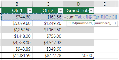
In this case we entered =sum(, then selected the Qtr 1 and Qtr 2 columns. As a result, Excel built the formula: =SUM(Table1[@[Qtr 1]:[Qtr 2]]). This is called a structured reference formula, which is unique to Excel tables. The structured reference format is what allows the table to use the same formula for each row. A regular Excel formula for this would be =SUM(B2:C2), which you would then need to copy or fill down to the rest of the cells in your column
To learn more about structured references, see: Using structured references with Excel tables.
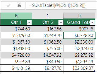
When you press Enter, the formula is automatically filled into all cells of the column — above as well as below the cell where you entered the formula. The formula is the same for each row, but since it’s a structured reference, Excel knows internally which row is which.
Copying or filling a formula into all cells of a blank table column also creates a calculated column.
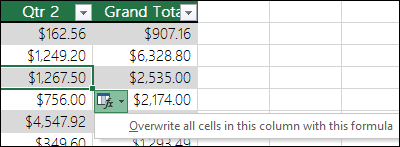
If you type or move a formula in a table column that already contains data, a calculated column is not automatically created. However, the AutoCorrect Options button is displayed to provide you with the option to overwrite the data so that a calculated column can be created.
If you input a new formula that is different from existing formulas in a calculated column, the column will automatically update with the new formula. You can choose to undo the update, and only keep the single new formula from the AutoCorrect Options button. This is generally not recommended though, because it can prevent your column from automatically updating in the future, since it won’t know which formula to extend when new rows are added.
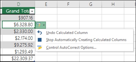
If you typed or copied a formula into a cell of a blank column and don’t want to keep the new calculated column, click Undo  twice. You can also press Ctrl + Z twice
A calculated column can include a cell that has a different formula from the rest. This creates an exception that will be clearly marked in the table. This way, inadvertent inconsistencies can easily be detected and resolved.
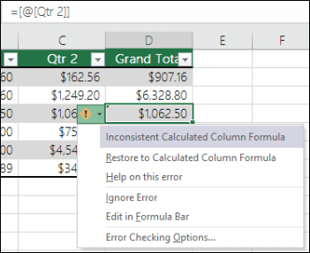
Note: Calculated column exceptions are created when you do any of the following:
Type data other than a formula in a calculated column cell.
Type a formula in a calculated column cell, and then click Undo on the Quick Access Toolbar.
Type a new formula in a calculated column that already contains one or more exceptions.
Copy data into the calculated column that does not match the calculated column formula.
Note: If the copied data contains a formula, this formula will overwrite the data in the calculated column.
Delete a formula from one or more cells in the calculated column.
Note: This exception is not marked.
Move or delete a cell on another worksheet area that is referenced by one of the rows in a calculated column.
Error notification will only appear if you have the background error checking option enabled. If you don’t see the error, then go to File > Options > Formulas > make sure the Enable background error checking box is checked.
If you’re using Excel 2007, click the Office button  , then Excel Options > Formulas.
If you’re using a Mac, go to Excel on the menu bar, and then click Preferences > Formulas & Lists > Error Checking.
The option to automatically fill formulas to create calculated columns in an Excel table is on by default. If you don’t want Excel to create calculated columns when you enter formulas in table columns, you can turn the option to fill formulas off. If you don’t want to turn the option off, but don’t always want to create calculated columns as you work in a table, you can stop calculated columns from being created automatically.
Turn calculated columns on or off
On the File tab, click Options.
If you’re using Excel 2007, click the Office button , then Excel Options.
Under AutoCorrect options, click AutoCorrect Options.
Click the AutoFormat As You Type tab.
Under Automatically as you work, select or clear the Fill formulas in tables to create calculated columns check box to turn this option on or off.
 Options > Proofing Tools > AutoCorrect Options > Uncheck «Fill formulas in tables to create calculated columns».» loading=»lazy»>
Tip: You can also click the AutoCorrect Options button that is displayed in the table column after you enter a formula. Click Control AutoCorrect Options, and then clear the Fill formulas in tables to create calculated columns check box to turn this option off.
If you’re using a Mac, goto Excel on the main menu, then Preferences > Formulas and Lists > Tables & Filters > Automatically fill formulas.
Stop creating calculated columns automatically
After entering the first formula in a table column, click the AutoCorrect Options button that is displayed, and then click Stop Automatically Creating Calculated Columns.
You can also create custom calculated fields with PivotTables, where you create one formula and Excel then applies it to an entire column. Learn more about Calculating values in a PivotTable.
Need more help?
You can always ask an expert in the Excel Tech Community or get support in the Answers community.
Источник