Application match in vba excel

Excel VBA Match Function

VBA Match Function looks for the position or row number of the lookup value in the table array i.e. in the main excel table. For example, VLOOKUP, HLOOKUP, MATCH, INDEX, etc. These are the lookup functions that are more important than others. Regretfully, we don’t have the same functions available in VBA for making things easier. However, we can use these functions as worksheet functions under the VBA script to make our lives easier.

Today, we are about to learn the MATCH function which can be used as a worksheet function under VBA.

VBA Match has the same use as the Match formula in Excel. This function in MS Excel VBA finds a match within an array with reference to the lookup value and prints its position. This function becomes useful when you need to evaluate the data based on certain values. For example, VBA MATCH is helpful if you have the salary data of employees and you need to find out the numeric position of an employee in your data who has salary less than/greater than/equals to a certain value. It is really helpful in analyzing the data and also one line of code can automate the things for you.

Syntax of Match Function in Excel VBA

VBA Match has the following syntax:

Where,

Arg1 – Lookup_value – The value you need to lookup in a given array.
Arg2 – Lookup_array – an array of rows and columns which contain possible Lookup_value.
Arg3 – Match_type – The match type which takes value -1, 0 or 1.

If match_type = -1 means that the MATCH function will find out the smallest value which is greater than or equals to the lookup_value. For this to happen, the lookup_array must be sorted in descending order.

If match_type = 0 means that the MATCH function will find out the value which is exactly the same as that of the lookup_value.

If match_type = +1 it means that the MATCH function will find out the largest value which is lesser than or equals to the lookup_value. For this to happen, the lookup_array must be sorted in ascending order. The default value for the match type is +1.

How to Use Excel VBA Match Function?

We will learn how to use a VBA Match Excel function with few examples.

You can download this VBA Match Excel Template here – VBA Match Excel Template

VBA Match Function – Example #1

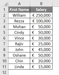
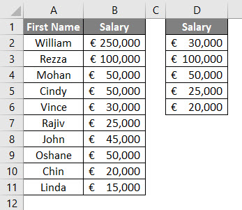
Suppose we have data as shown below:

We need to find who from this list have salary € 30,000 along with position in Excel.

Though in this data set we can manually configure this, please think on a broader picture, what if you have millions of rows and columns?

Follow the below steps to use MATCH function in VBA.

Step 1: Define a sub-procedure by giving a name to macro.

Code:

Sub exmatch1()

End Sub

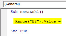
Step 2: Now, we want our output to be stored in cell E2. Therefore, start writing the code as Range(“E2”).Value =

This defines the output range for our result.

Code:

Sub exmatch1()

  Range("E2").Value =

End Sub

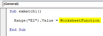
Step 3: Use WorksheetFunction to be able to use VBA functions.

Code:

Sub exmatch1()

  Range("E2").Value = WorksheetFunction

End Sub

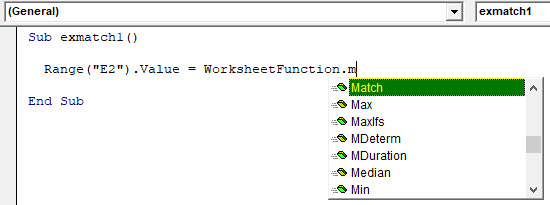
Step 4: WorksheetFunction has a variety of functions that can be accessed and used under VBA. After “WorksheetFunction”, put a dot (.) and then you’ll be able to access the functions. Choose the MATCH function from the dropdown list.

Code:

Sub exmatch1()

  Range("E2").Value = WorksheetFunction.Match

End Sub

Step 5: Now, give the arguments to the MATCH function. Like Lookup_value. Our Lookup_value is stored in cell D2 as shown in the below screenshot. You can access it under the MATCH function using Range function.

Code:

Sub exmatch1()

  Range("E2").Value = WorksheetFunction.Match(Range("D2").Value,

End Sub

Step 6: The Second argument is Lookup_array. This is the table range within which you want to find out the position of Lookup_value. In our case, it is (B1:B11). Provide this array using the Range function.

Code:

Sub exmatch1()

  Range("E2").Value = WorksheetFunction.Match(Range("D2").Value, Range("B1:B11"),

End Sub

Step 7: The Last argument for this code to work out is Match_type. We wanted to have an exact match for Lookup_value in given range> Therefore, give Zero (0) as a matching argument.

Code:

Sub exmatch1()

  Range("E2").Value = WorksheetFunction.Match(Range("D2").Value, Range("B1:B11"), 0)

End Sub

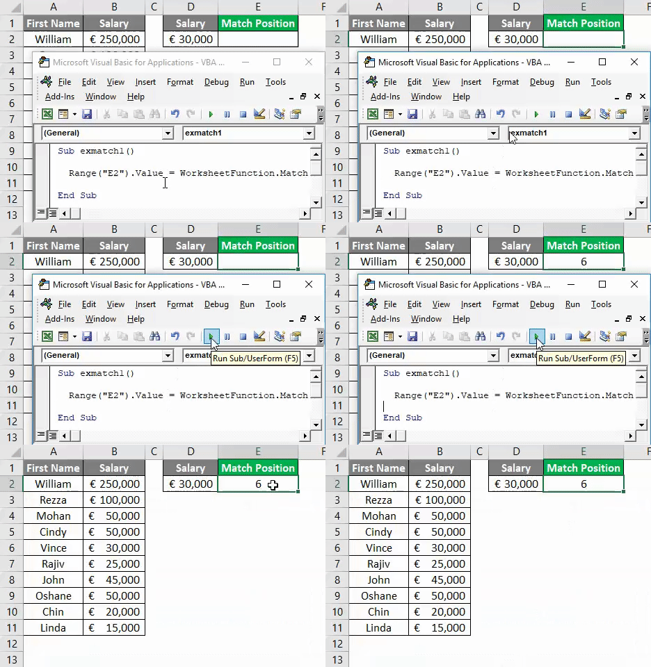
Step 8: Run this code by hitting F5 or Run button and see the output.

You can see in Cell E2, there is a numeric value (6) which shows the position of the value from cell D2 through range B1:B11.

Example #2 – VBA Match Function with Loops

It is easy when you have only one value to lookup for in the entire range. But, what if you need to check the position for a number of cells? It would be harsh on a person who is adding to ask him to write the separate codes for each cell.

In such cases, MATCH function can be used with loop (especially For loop in our case). See the following steps to get an idea of how we use MATCH function with loop.

Step 1: Define a subprocedure by giving a name to macro.

Code:

Sub Example2()

End Sub

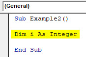
Step 2: Define an integer that can hold the value for multiple cells in the loop.

Code:

Sub Example2()

Dim i As Integer

End Sub

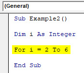
Step 3: Use For loop on the integer to use the different lookup values whose position can be stored in column E.

Code:

Sub Example2()

Dim i As Integer

For i = 2 To 6

End Sub

Step 4: Now, use the same method we used in example 1, just instead of Range, we will use the Cells function and will be using a two-dimensional array (Rows and columns) in contrast to the first example.

Code:

Sub Example2()

Dim i As Integer

For i = 2 To 6
Cells(i, 5).Value = WorksheetFunction.Match(Cells(i, 4).Value, Range("B2:B11"), 0)
Next i

End Sub

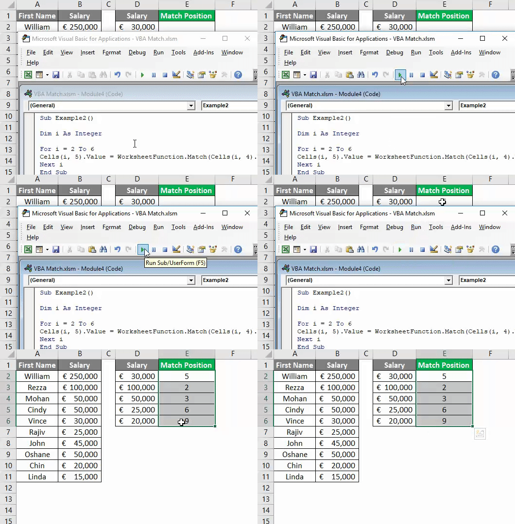
Here, Cells(i, 5).Value = stores the value of resulting positions in each row from 2 to 6 (row i) in column E (column number 5). Under Match function, Cells(i, 4).Values checks for each Lookup_value present in row 2 to 6 in the 4^th column. This lookup value then searched in Array B2:B11 in excel sheet where data is present and relative positions can be stored in each row of column 5 (column E).

Step 5: Run this code by hitting F5 or Run button simultaneously and see the result. It will almost pull out the magic in a piece of code with a single line.

In this article, we learned how we can use MATCH function under VBA as a special case of WorksheetFunction.

Things to Remember

Lookup_value can be number/text/logical value or can be a cell reference to a number, text or logical value.
By default, Match_type can be considered as 1, if omitted/not mentioned.
As similar to Excel MATCH function, VBA MATCH also gives the relative position of a Lookup_value under Lookup_array and not the value itself.
If a match is not found, a relative excel cell will be filled with #N/A.
If MATCH function is used on Text values, it is not able to differentiate between lowercases and uppercases. For Example, Lalit and lalit are same. So do LALIT and lalit.
Wildcard characters can be used if you are finding out the exact match (i.e. match type is zero). Wildcard character asterisk (*) can be used to find out a series of characters. While a question mark (?) can be used to find out a single character.

Quick Recap of MATCH Function

The MATCH function is a lookup functionThe LOOKUP excel function searches a value in a range (single row or single column) and returns a corresponding match from the same position of another range (single row or single column). The corresponding match is a piece of information associated with the value being searched.
read more that looks for the position of the lookup value in the mentioned lookup array. For example, look at the below image of the data.

In the above data, we have months from A2 to A6. If we want to know where “Mar” month occurs, we can use the MATCH function.

Below is the syntax of the MATCH functionThe MATCH function looks for a specific value and returns its relative position in a given range of cells. The output is the first position found for the given value. Being a lookup and reference function, it works for both an exact and approximate match. For example, if the range A11:A15 consists of the numbers 2, 9, 8, 14, 32, the formula “MATCH(8,A11:A15,0)” returns 3. This is because the number 8 is at the third position.
read more.

MATCH (Lookup Value, Lookup Array, [Match Type])

Lookup Value: For which value we are looking for the position in the lookup array.
Lookup Array: In which array we are looking for the position of the lookup value.
[Match Type]: For this, we can provide three arguments.

1 = Less Than
0 = Exact Match
-1 = Greater Than

Most of the time, we use only “0 Exact Match”.

You can download this VBA Application.Match Excel Template here – VBA Application.Match Excel Template

How to Use Application.Match Function in VBA?

Example #1

Look at the below data in excel.

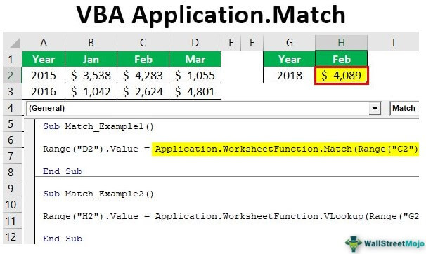
We need to find the position of the “Mar” month in the range of cells from A2 to A6. Since we need results in D2 cells, start the code as Range(“D2”).Value =.

We need to use the MATCH worksheet function to arrive at the value in the D2 cell. So, to access this first, we need to access the APPLICATION object and then the WORKSHEET FUNCTIONThe worksheet function in VBA is used when we need to refer to a specific worksheet. When we create a module, the code runs in the currently active sheet of the workbook, but we can use the worksheet function to run the code in a particular worksheet.read more object.

Enter dot to see a list of worksheet functions.

Choose “Match” from the list.

One of the problems in VBA while using worksheet functions is we do not see exact syntax as we see with worksheet functions. It is one of the reasons we have explained the syntax at the beginning only.

So, the first argument is lookup value, i.e., for which value we are looking to find the place. In this case, we are looking to find the place for “Mar,” which is in the C2 cell, so supply the cell referenceCell reference in excel is referring the other cells to a cell to use its values or properties. For instance, if we have data in cell A2 and want to use that in cell A1, use =A2 in cell A1, and this will copy the A2 value in A1.read more.

The next argument is the lookup array, i.e., in which range we are looking for the position of a lookup value. For this, supply cells from A2 to A6.

The last argument will be an exact match, so supply 0.

Code:

Sub Match_Example1()
Range("D2").Value = Application.WorksheetFunction.Match(Range("C2").Value, Range("A2:A6"), 0)
End Sub

We have finished with the formula.

Run the code through the F5 key and see what we get.

So, we got the result as 3 because the value “Mar” is in the third position in the range A2 to A6.

This MATCH function can provide the position of the lookup value. However, the MATCH function is largely used with the VLOOKUP functionThe VLOOKUP excel function searches for a particular value and returns a corresponding match based on a unique identifier. A unique identifier is uniquely associated with all the records of the database. For instance, employee ID, student roll number, customer contact number, seller email address, etc., are unique identifiers.
read more to supply the column index number based on the column header.

Example #2

Now, we will see how to use MATCH as a supporting function for the VLOOKUP function.

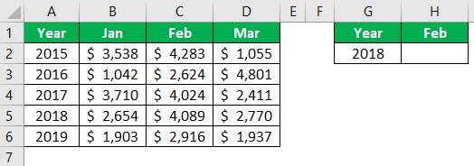
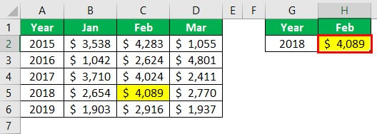
Look at the below data.

In the above table, we are looking at the year 2018 “Feb” month sales, so we need to use the VLOOKUP function. VLOOKUP is also a worksheet function, so access this like how we have accessed the MATCH function.

Lookup Value will be G2 cell, so supply cell address.

Code:

Sub Match_Example2()
Range("H2").Value = Application.WorksheetFunction.VLookup(Range("G2").Value,
End Sub

Table Array will be from A2 to D6.

Code:

Sub Match_Example2()
Range("H2").Value = Application.WorksheetFunction.VLookup(Range("G2").Value,Range("A2:D6"),
End Sub

Now, we need to provide the result from which column of the table array we are looking for. So, this will be from the third column. Instead of supplying the column number as 3, let us use the MATCH function.

Code:

Sub Match_Example2()
Range("H2").Value = Application.WorksheetFunction.VLookup(Range("G2").Value, Range("A2:D6"), Application.WorksheetFunction.Match(Range("H1").Value, Range("A1:D1"), 0), 0)
End Sub

So, the MATCH function provides the column number from the range A1 to D1 for the month “Feb.” Let us run the code and see how it gets column numbers automatically.

We have column number 2, thanks to the MATCH function’s automatic column number supply.

Things to Remember

The MATCH function looks for the position of the lookup value in the selected array table.
The MATCH function is mainly used with the VLOOKUP function to supply the column index number using the column heading automatically.
The MATCH function is available as a worksheet function in VBA.

Синтаксис

Синтаксис метода WorksheetFunction.Match в VBA Excel:

WorksheetFunction.Match (Arg1, Arg2, [Arg3])

Параметры

Описание параметров метода WorksheetFunction.Match:

Параметр	Описание
Arg1	Обязательный параметр. Значение элемента массива, по которому будет произведен поиск относительного положения элемента в массиве.
Arg2	Обязательный параметр. Непрерывный диапазон ячеек или массив, в котором будет произведен поиск позиции элемента, значение которого совпадет со значением параметра Arg1.
Arg3	Необязательный параметр. Задает тип сопоставления значения Arg1 со значениями в массиве Arg2.

В параметре Arg1 можно использовать знаки подстановки для шаблонов, те же, что и для методов Find и Replace.

Значения параметра Arg3, задающие тип сопоставления:

Значение	Тип сопоставления
-1	Метод WorksheetFunction.Match находит наименьшее значение элемента в Arg2, большее или равное Arg1. Значения элементов Arg2 должны быть расположены в убывающем порядке: [m, … 2, 1, 0, -1, -2, … -n], [z – a], [True, False] и т. д.
0	Метод WorksheetFunction.Match находит в Arg2 первое значение, равное Arg1. Значения элементов Arg2 могут быть расположены в любом порядке.
1	Значение по умолчанию. Метод WorksheetFunction.Match находит наибольшее значение элемента в Arg2, меньшее или равное Arg1. Значения элементов Arg2 должны быть расположены в возрастающем порядке: [-n, … -2, -1, 0, 1, 2, … m], [a – z], [False, True] и т. д.

При сопоставлении строк регистр не учитывается.

Примеры

Пример 1

Поиск относительного положения элемента в массиве, индексация которого начинается с нуля:

Sub Primer1()

Dim myArray As Variant, n As Long

‘заполнение массива значениями, нумерация элементов массива начинается с нуля

myArray = Array(«Арка», 45, «Дуб», «Клуб», 85.37, «Литр», 103, «Небо», «Столб»)

‘определяем относительное положение элемента в массиве, при чем

‘нумерация относительного положения начинается с единицы

n = WorksheetFunction.Match(«Клуб», myArray)

MsgBox n ‘Результат: 4

MsgBox myArray(n) ‘Результат: 85.37, так как нумерация массива начинается с нуля

End Sub

Пример 2

Определение индекса элемента в массиве по его относительному положению, возвращенному методом WorksheetFunction.Match:

Sub Primer2()

Dim myArray(7 To 15) As Variant, i As Long, n As Long

‘заполнение элементов массива значениями

For i = 7 To 15

myArray(i) = Choose(i, «», «», «», «», «», «», «Арка», 45, «Дуб», «Клуб», 85.37, «Литр», 103, «Небо», «Столб»)

n = WorksheetFunction.Match(«Клуб», myArray)

MsgBox n ‘Результат: 4

‘находим индекс элемента в массиве по его относительному положению

n = n + LBound(myArray) — 1

MsgBox myArray(n) ‘Результат: Клуб

End Sub

Пример 3

Определение адреса ячейки на рабочем листе по найденному методом WorksheetFunction.Match относительному положению этой ячейки в заданном диапазоне:

Sub Primer3()

Dim n As Long

n = WorksheetFunction.Match(«Брелок», Range(«B1400:B1410»), 0)

With Range(«B1400:B1410»)

MsgBox «Значение = « & .Cells(n) & vbNewLine & _

«Адрес = « & .Cells(n).Address & vbNewLine & _

«Строка = « & .Cells(n).Row & vbNewLine & _

«Столбец = « & .Cells(n).Column

End With

End Sub

Источник

title	keywords	f1_keywords	ms.prod	api_name	ms.assetid	ms.date	ms.localizationpriority
WorksheetFunction.Match method (Excel)	vbaxl10.chm137114	vbaxl10.chm137114	excel	Excel.WorksheetFunction.Match	901cdd78-e8fc-f149-66ff-5887f7099c96	05/24/2019	medium

WorksheetFunction.Match method (Excel)

Returns the relative position of an item in an array that matches a specified value in a specified order. Use Match instead of one of the Lookup functions when you need the position of an item in a range instead of the item itself.

Syntax

expression.Match (Arg1, Arg2, Arg3)

expression A variable that represents a WorksheetFunction object.

Parameters

Name	Required/Optional	Data type	Description
Arg1	Required	Variant	Lookup_value: the value that you use to find the value that you want in a table.
Arg2	Required	Variant	Lookup_array: a contiguous range of cells containing possible lookup values. Lookup_array must be an array or an array reference.
Arg3	Optional	Variant	Match_type: the number -1, 0, or 1. Match_type specifies how Microsoft Excel matches lookup_value with values in lookup_array.

Return value

Double

Remarks

Lookup_value is the value that you want to match in lookup_array. For example, when you look up a number in a telephone book, you are using the person’s name as the lookup value, but the telephone number is the value that you want.

Lookup_value can be a value (number, text, or logical value) or a cell reference to a number, text, or logical value.

If match_type is 1, Match finds the largest value that is less than or equal to lookup_value. Lookup_array must be placed in ascending order: …-2, -1, 0, 1, 2, …, A-Z, FALSE, TRUE.

If match_type is 0, Match finds the first value that is exactly equal to lookup_value. Lookup_array can be in any order. Note that Match is case-insensitive.

If match_type is -1, Match finds the smallest value that is greater than or equal to lookup_value. Lookup_array must be placed in descending order: TRUE, FALSE, Z-A, …2, 1, 0, -1, -2, …, and so on.

If match_type is omitted, it is assumed to be 1.

Match returns the position of the matched value within lookup_array, not the value itself. For example, MATCH("b",{"a","b","c"},0) returns 2, the relative position of «b» within the array {"a","b","c"}.

Match does not distinguish between uppercase and lowercase letters when matching text values.

If Match is unsuccessful in finding a match, it returns the #N/A error value.

If match_type is 0 and lookup_value is text, you can use the wildcard characters, question mark (?) and asterisk (*), in lookup_value. A question mark matches any single character; an asterisk matches any sequence of characters. If you want to find an actual question mark or asterisk, type a tilde (~) before the character.

Example

For each value in the first column of the first worksheet, this example searches through the entire workbook for a matching value. If the macro finds a matching value, it sets the original value on the first worksheet to be bold.

Sub HighlightMatches()
    Application.ScreenUpdating = False
    
    'Declare variables
    Dim var As Variant, iSheet As Integer, iRow As Long, iRowL As Long, bln As Boolean
       
       'Set up the count as the number of filled rows in the first column of Sheet1.
       iRowL = Cells(Rows.Count, 1).End(xlUp).Row
       
       'Cycle through all the cells in that column:
       For iRow = 1 To iRowL
          'For every cell that is not empty, search through the first column in each worksheet in the
          'workbook for a value that matches that cell value.

          If Not IsEmpty(Cells(iRow, 1)) Then
             For iSheet = ActiveSheet.Index + 1 To Worksheets.Count
                bln = False
                var = Application.Match(Cells(iRow, 1).Value, Worksheets(iSheet).Columns(1), 0)
                
                'If you find a matching value, indicate success by setting bln to true and exit the loop;
                'otherwise, continue searching until you reach the end of the workbook.
                If Not IsError(var) Then
                   bln = True
                   Exit For
                End If
             Next iSheet
          End If
          
          'If you don't find a matching value, don't bold the value in the original list;
          'if you do find a value, bold it.
          If bln = False Then
             Cells(iRow, 1).Font.Bold = False
             Else
             Cells(iRow, 1).Font.Bold = True
          End If
       Next iRow
    Application.ScreenUpdating = True
End Sub

[!includeSupport and feedback]

Источник

Date yes Add (Subtract) Days to a Date Concatenate Dates Convert Date to Number Convert Date to Text Month Name to Number Create Date Range from Dates Day Number of Year Month Name from Date First Day of Month Add (Subtract) Weeks to a Date If Functions with Dates Max Date Number of Days Between Dates Number of Days in a Month Number of Weeks Between Dates Number of Years Between Dates Split Date & Time into Separate Cells Countdown Remaining Days Insert Dates Random Date Generator Using Dynamic Ranges — Year to Date Values Add (Subtract) Years to a Date Date Formula Examples Extract Day from Date Get Day Name from Date Count Days Left in Month / Year Count Workdays Left in Month / Year Get Last Day of Month Last Business Day of Month / Year Number of Work / Business Days in Month Weekday Abbreviations Auto Populate Dates Number of Months Between Dates Quarter from a Date Years of Service Change Date Format Compare Dates Time yes Add (Subtract) Hours to Time Add (Subtract) Minutes to Time Add (Subtract) Seconds to Time Add Up time (Total Time) Time Differences Change Time Format Convert Minutes to Hours Convert Time to Decimal Convert Time to Hours Convert Time to Minutes Convert Time to Seconds Military Time Round Time to Nearest 15 Minutes Overtime Calculator Number of Hours Between Times Convert Seconds to Minutes, Hours, or Time Count Hours Worked Time Differences Time Format — Show Minutes Seconds Text yes Add Commas to Cells Get First Word from Text Capitalize First Letter Clean & Format Phone #s Remove Extra Trailing / Leading Spaces Add Spaces to Cell Assign Number Value to Text Combine Cells with Comma Combine First and Last Names Convert Text String to Date Convert Text to Number Extract Text From Cell Get Last Word Remove Unwated Characters Extract Text Before or After Character How to Split Text String by Space, Comma, & More Remove Special Characters Remove First Characters from Left Substitute Multiple Values Switch First & Last Names w/ Commas Remove Specific Text from a Cell Extract Text Between Characters (Ex. Parenthesis) Add Leading Zeros to a Number Remove Line Breaks from Text Remove all Numbers from Text Reverse Text Remove Non-Numeric Characters Remove Last Character(s) From Right Separate First and Last Names Separate Text & Numbers Round yes Round Formulas Round Price to Nearest Dollar or Cent Round to Nearest 10, 100, or 1000 Round to Nearest 5 or .5 Round Percentages Round to Significant Figures Count yes Count Blank and Non-blank Cells Count Cells Between Two Numbers Count Cells not Equal to Count if Cells are in Range Count Times Word Appears in Cell Count Words in Cell Count Specific Characters in Column Count Total Number of Characters in Column Count Cells that Equal one of two Results Count Cells that do not Contain Count Cells that Contain Specific Text Count Unique Values in Range Countif — Multiple Criteria Count Total Number of Cells in Range Count Cells with Any Text Count Total Cells in a Table Lookup yes Two Dimensional VLOOKUP VLOOKUP Simple Example Vlookup — Multiple Matches Case Sensitive Lookup Case Sensitive VLOOKUP Sum if — VLOOKUP Case Sensitive Lookup Case Sensitive VLOOKUP Find Duplicates w/ VLOOKUP or MATCH INDEX MATCH MATCH Lookup — Return Cell Address (Not Value) Lookup Last Value in Column or Row Reverse VLOOKUP (Right to Left) Risk Score Bucket with VLOOKUP Sum with a VLOOKUP Function VLOOKUP & INDIRECT VLOOKUP Concatenate VLOOKUP Contains (Partial Match) 17 Reasons Why Your XLOOKUP is Not Working Double (Nested) XLOOKUP — Dynamic Columns IFERROR (& IFNA) XLOOKUP Lookup Min / Max Value Nested VLOOKUP Top 11 Alternatives to VLOOKUP (Updated 2022!) VLOOKUP – Dynamic Column Reference VLOOKUP – Fix #N/A Error VLOOKUP – Multiple Sheets at Once VLOOKUP & HLOOKUP Combined VLOOKUP & MATCH Combined VLOOKUP Between Worksheets or Spreadsheets VLOOKUP Duplicate Values VLOOKUP Letter Grades VLOOKUP Return Multiple Columns VLOOKUP Returns 0? Return Blank Instead VLOOKUP w/o #N/A Error XLOOKUP Multiple Sheets at Once XLOOKUP Between Worksheets or Spreadsheets XLOOKUP by Date XLOOKUP Duplicate Values XLOOKUP Multiple Criteria XLOOKUP Return Multiple Columns XLOOKUP Returns 0? Return Blank Instead XLOOKUP Text XLOOKUP with IF XLOOKUP With If Statement Misc. yes Sort Multiple Columns Use Cell Value in Formula Percentage Change Between Numbers Percentage Breakdown Rank Values Add Spaces to Cell CAGR Formula Average Time Decimal Part of Number Integer Part of a Number Compare Items in a List Dealing with NA() Errors Get Worksheet Name Wildcard Characters Hyperlink to Current Folder Compound Interest Formula Percentage Increase Create Random Groups Sort with the Small and Large Functions Non-volatile Function Alternatives Decrease a Number by a Percentage Calculate Percent Variance Profit Margin Calculator Convert Column Number to Letter Get Full Address of Named Range Insert File Name Insert Path Latitute / Longitude Functions Replace Negative Values Reverse List Range Convert State Name to Abbreviation Create Dynamic Hyperlinks Custom Sort List with Formula Data Validation — Custom Formulas Dynamic Sheet Reference (INDIRECT) Reference Cell in Another Sheet or Workbook Get Cell Value by Address Get Worksheet Name Increment Cell Reference List Sheet Names List Skipped Numbers in Sequence Return Address of Max Value in Range Search by Keywords Select Every Other (or Every nth) Row Basics yes Cell Reference Basics — A1, R1C1, 3d, etc. Add Up (Sum) Entire Column or Row Into to Dynamic Array Formulas Conversions yes Convert Time Zones Convert Celsius to Fahrenheit Convert Pounds to Kilograms Convert Time to Unix Time Convert Feet to Meters Convert Centimeters to Inches Convert Kilometers to Miles Convert Inches to Feet Convert Date to Julian Format Convert Column Letter to Number Tests yes Test if a Range Contains any Text Test if any Cell in Range is Number Test if a Cell Contains a Specific Value Test if Cell Contains Any Number Test if Cell Contains Specific Number Test if Cell is Number or Text If yes Percentile If Subtotal If Sumproduct If Large If and Small If Median If Concatentate If Max If Rank If TEXTJOIN If Sum yes Sum if — Begins With / Ends With Sum if — Month or Year to Date Sum if — By Year Sum if — Blank / Non-Blank Sum if — Horizontal Sum Count / Sum If — Cell Color INDIRECT Sum Sum If — Across Multiple Sheets Sum If — By Month Sum If — Cells Not Equal To Sum If — Not Blank Sum if — Between Values Sum If — Week Number Sum Text Sum if — By Category or Group Sum if — Cell Contains Specific Text (Wildcards) Sum if — Date Rnage Sum if — Dates Equal Sum if — Day of Week Sum if — Greater Than Sum if — Less Than Average yes Average Non-Zero Values Average If — Not Blank Average — Ignore 0 Average — Ignore Errors Math yes Multiplication Table Cube Roots nth Roots Square Numbers Square Roots Calculations yes Calculate a Ratio Calculate Age KILLLLLLL Calculate Loan Payments GPA Formula Calculate VAT Tax How to Grade Formulas Find yes Find a Number in a Column / Workbook Find Most Frequent Numbers Find Smallest n Values Find nth Occurance of Character in Text Find and Extract Number from String Find Earliest or Latest Date Based on Criteria Find First Cell with Any Value Find Last Row Find Last Row with Data Find Missing Values Find Largest n Values Most Frequent Number Conditional Formatting yes Conditional Format — Dates & Times Conditional Format — Highlight Blank Cells New Functions XLOOKUP Replaces VLOOKUP, HLOOKUP, and INDEX / MATCH Logical yes AND Checks whether all conditions are met. TRUE/FALSE IF If condition is met, do something, if not, do something else. IFERROR If result is an error then do something else. NOT Changes TRUE to FALSE and FALSE to TRUE. OR Checks whether any conditions are met. TRUE/FALSE XOR Checks whether one and only one condition is met. TRUE/FALSE Lookup & Reference yes FALSE The logical value: FALSE. TRUE The logical value: TRUE. ADDRESS Returns a cell address as text. AREAS Returns the number of areas in a reference. CHOOSE Chooses a value from a list based on it’s position number. COLUMN Returns the column number of a cell reference. COLUMNS Returns the number of columns in an array. HLOOKUP Lookup a value in the first row and return a value. HYPERLINK Creates a clickable link. INDEX Returns a value based on it’s column and row numbers. INDIRECT Creates a cell reference from text. LOOKUP Looks up values either horizontally or vertically. MATCH Searches for a value in a list and returns its position. OFFSET Creates a reference offset from a starting point. ROW Returns the row number of a cell reference. ROWS Returns the number of rows in an array. TRANSPOSE Flips the oriention of a range of cells. VLOOKUP Lookup a value in the first column and return a value. Date & Time yes DATE Returns a date from year, month, and day. DATEDIF Number of days, months or years between two dates. DATEVALUE Converts a date stored as text into a valid date DAY Returns the day as a number (1-31). DAYS Returns the number of days between two dates. DAYS360 Returns days between 2 dates in a 360 day year. EDATE Returns a date, n months away from a start date. EOMONTH Returns the last day of the month, n months away date. HOUR Returns the hour as a number (0-23). MINUTE Returns the minute as a number (0-59). MONTH Returns the month as a number (1-12). NETWORKDAYS Number of working days between 2 dates. NETWORKDAYS.INTL Working days between 2 dates, custom weekends. NOW Returns the current date and time. SECOND Returns the second as a number (0-59) TIME Returns the time from a hour, minute, and second. TIMEVALUE Converts a time stored as text into a valid time. TODAY Returns the current date. WEEKDAY Returns the day of the week as a number (1-7). WEEKNUM Returns the week number in a year (1-52). WORKDAY The date n working days from a date. WORKDAY.INTL The date n working days from a date, custom weekends. YEAR Returns the year. YEARFRAC Returns the fraction of a year between 2 dates. Engineering yes CONVERT Convert number from one unit to another. Financial yes FV Calculates the future value. PV Calculates the present value. NPER Calculates the total number of payment periods. PMT Calculates the payment amount. RATE Calculates the interest Rate. NPV Calculates the net present value. IRR The internal rate of return for a set of periodic CFs. XIRR The internal rate of return for a set of non-periodic CFs. PRICE Calculates the price of a bond. YIELD Calculates the bond yield. INTRATE The interest rate of a fully invested security. Information yes CELL Returns information about a cell. ERROR.TYPE Returns a value representing the cell error. ISBLANK Test if cell is blank. TRUE/FALSE ISERR Test if cell value is an error, ignores #N/A. TRUE/FALSE ISERROR Test if cell value is an error. TRUE/FALSE ISEVEN Test if cell value is even. TRUE/FALSE ISFORMULA Test if cell is a formula. TRUE/FALSE ISLOGICAL Test if cell is logical (TRUE or FALSE). TRUE/FALSE ISNA Test if cell value is #N/A. TRUE/FALSE ISNONTEXT Test if cell is not text (blank cells are not text). TRUE/FALSE ISNUMBER Test if cell is a number. TRUE/FALSE ISODD Test if cell value is odd. TRUE/FALSE ISREF Test if cell value is a reference. TRUE/FALSE ISTEXT Test if cell is text. TRUE/FALSE N Converts a value to a number. NA Returns the error: #N/A. TYPE Returns the type of value in a cell. Math yes ABS Calculates the absolute value of a number. AGGREGATE Define and perform calculations for a database or a list. CEILING Rounds a number up, to the nearest specified multiple. COS Returns the cosine of an angle. DEGREES Converts radians to degrees. DSUM Sums database records that meet certain criteria. EVEN Rounds to the nearest even integer. EXP Calculates the exponential value for a given number. FACT Returns the factorial. FLOOR Rounds a number down, to the nearest specified multiple. GCD Returns the greatest common divisor. INT Rounds a number down to the nearest integer. LCM Returns the least common multiple. LN Returns the natural logarithm of a number. LOG Returns the logarithm of a number to a specified base. LOG10 Returns the base-10 logarithm of a number. MOD Returns the remainder after dividing. MROUND Rounds a number to a specified multiple. ODD Rounds to the nearest odd integer. PI The value of PI. POWER Calculates a number raised to a power. PRODUCT Multiplies an array of numbers. QUOTIENT Returns the integer result of division. RADIANS Converts an angle into radians. RAND Calculates a random number between 0 and 1. RANDBETWEEN Calculates a random number between two numbers. ROUND Rounds a number to a specified number of digits. ROUNDDOWN Rounds a number down (towards zero). ROUNDUP Rounds a number up (away from zero). SIGN Returns the sign of a number. SIN Returns the sine of an angle. SQRT Calculates the square root of a number. SUBTOTAL Returns a summary statistic for a series of data. SUM Adds numbers together. SUMIF Sums numbers that meet a criteria. SUMIFS Sums numbers that meet multiple criteria. SUMPRODUCT Multiplies arrays of numbers and sums the resultant array. TAN Returns the tangent of an angle. TRUNC Truncates a number to a specific number of digits. Stats yes AVERAGE Averages numbers. AVERAGEA Averages numbers. Includes text & FALSE =0, TRUE =1. AVERAGEIF Averages numbers that meet a criteria. AVERAGEIFS Averages numbers that meet multiple criteria. CORREL Calculates the correlation of two series. COUNT Counts cells that contain a number. COUNTA Count cells that are non-blank. COUNTBLANK Counts cells that are blank. COUNTIF Counts cells that meet a criteria. COUNTIFS Counts cells that meet multiple criteria. FORECAST Predict future y-values from linear trend line. FREQUENCY Counts values that fall within specified ranges. GROWTH Calculates Y values based on exponential growth. INTERCEPT Calculates the Y intercept for a best-fit line. LARGE Returns the kth largest value. LINEST Returns statistics about a trendline. MAX Returns the largest number. MEDIAN Returns the median number. MIN Returns the smallest number. MODE Returns the most common number. PERCENTILE Returns the kth percentile. PERCENTILE.INC Returns the kth percentile. Where k is inclusive. PERCENTILE.EXC Returns the kth percentile. Where k is exclusive. QUARTILE Returns the specified quartile value. QUARTILE.INC Returns the specified quartile value. Inclusive. QUARTILE.EXC Returns the specified quartile value. Exclusive. RANK Rank of a number within a series. RANK.AVG Rank of a number within a series. Averages. RANK.EQ Rank of a number within a series. Top Rank. SLOPE Calculates the slope from linear regression. SMALL Returns the kth smallest value. STDEV Calculates the standard deviation. STDEV.P Calculates the SD of an entire population. STDEV.S Calculates the SD of a sample. STDEVP Calculates the SD of an entire population TREND Calculates Y values based on a trendline. Text yes CHAR Returns a character specified by a code. CLEAN Removes all non-printable characters. CODE Returns the numeric code for a character. CONCATENATE Combines text together. DOLLAR Converts a number to text in currency format. EXACT Test if cells are exactly equal. Case-sensitive. TRUE/FALSE FIND Locates position of text within a cell.Case-sensitive. LEFT Truncates text a number of characters from the left. LEN Counts number of characters in text. LOWER Converts text to lower case. MID Extracts text from the middle of a cell. PROPER Converts text to proper case. REPLACE Replaces text based on it’s location. REPT Repeats text a number of times. RIGHT Truncates text a number of characters from the right. SEARCH Locates position of text within a cell.Not Case-sensitive. SUBSTITUTE Finds and replaces text. Case-sensitive. TEXT Converts a value into text with a specific number format. TRIM Removes all extra spaces from text. UPPER Converts text to upper case. VALUE Converts a number stored as text into a number.

Источник

Excel VBA Match Function

Syntax of Match Function in Excel VBA

How to Use Excel VBA Match Function?

VBA Match Function – Example #1

Example #2 – VBA Match Function with Loops

Things to Remember

Recommended Articles

Table of contents

Quick Recap of MATCH Function

How to Use Application.Match Function in VBA?

Example #1

Example #2

Things to Remember

Recommended Articles

Синтаксис

Параметры

Примеры

Пример 1

Пример 2

Пример 3

WorksheetFunction.Match method (Excel)

Syntax

Parameters

Return value

Remarks

Example