
This article will show you how to easily add/attach file like PDF, Word or any other to Excel spreadsheet.
Applies to: Excel, Excel 2013, Excel 2016, Excel 2019, Excel 365, Office 365
-
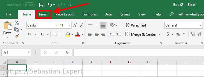
Go to Insert tab

Excel 2016/2019/365 — Home tab
-
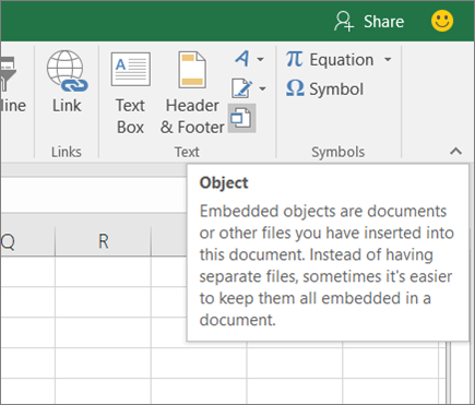
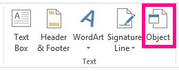
Click Object button placed in Text group.
Narrow window

Insert Object button — narrow window
Medium width window

Insert Object button — medium width window
Maximum width window
Insert Object button — max width window
-
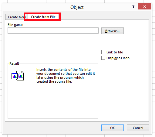
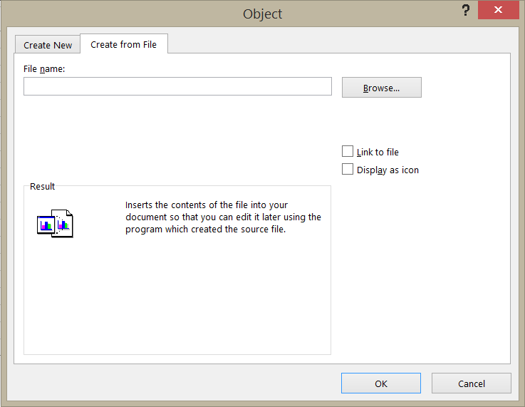
Click Create from file and browse for the file.

Click to enlarge


Skip to content
How to Insert Attachments in Excel?

Do you ever need to insert files into Excel, so you can share more comprehensive information with your colleagues? Either to insert PDF into Excel or to insert word documents into Excel, it’s just as simple as clicking on Insert, Text, Object, choosing your file, and voila!
Then, what happens after? Your file will float around your spreadsheet and not into a single cell. Yet, to be able to sort or move it with the rest of the content, what you really need is to put it into a single cell. How can you do this?
In this brief article, we will see how Excel can better handle your attachments, then we will look into an alternative that integrates with Excel: RowShare, an online table that offers a collaboration solution.
Insert Files into Excel Sheet
There are several ways to insert files into Excel sheet. You can either create from files, create new or add link to files. We will explore how to do it one by one.
If you want to create from an existing file, follow these steps:
- Select the cell into which you want to insert your file
- Click on the “Insert” tab
- Click on “Object” under the “Text” group
- Select “Create from File”
- Browse your file
- Select the “Display as icon” check box to if you want to insert an icon linking to the files
- Click on “OK”
Another possibility is to create a new file. You can do that by selecting “Create New” instead, and choose the type of object you want to attach. A new window will then pop up and you can create a new file you want to insert.
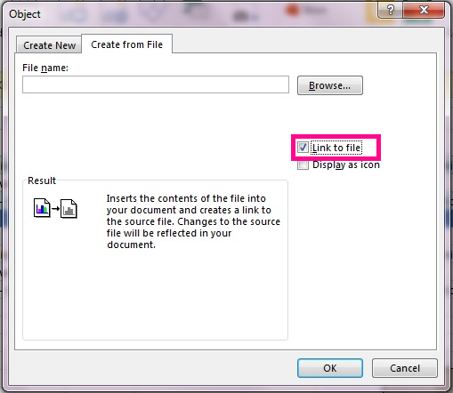
If you only want to add a link to the file instead of embedding the file, select the “Link to File” check box. The file should be stored in a location accessible to those with whom you want to share it. If the link to your file redirects to your computer, you will be the only one able to open it. Other than that, the location of the file should remain the same, if you move it to different location, the link won’t work anymore.
Attach Files in Excel, Within Excel Cells

Once you have made it to insert word documents into Excel or attach PDF to Excel, you probably realize that what you need is to insert your file into a single cell. To do this, follow these steps:
- Resize your file or cell until they fit each other
- Right click on your file and select “Format Object”
- Click on the “Properties” tab
- Select “Move and size with cells”
Since your Excel file size will be the size of the sheet itself plus the size of each other files attached, your Excel size will then be so huge. Also, as you can see here, there is no direct way to insert your file to an Excel cell automatically.
So, crunch time: Should I follow all these long endless steps or should I stick to the traditional way and exchange my files using email instead?
Attach Files Easily with RowShare
It’s time to say goodbye to complicated spreadsheet and endless email exchange. RowShare, an online table focusing in sharing and collaboration, offers a simpler solution. You can insert attachments within a click of a mouse! Start by creating a table from RowShare’s templates or from scratch.
Attach your files by following these super simple steps:
- Add a column of type “File” to your table
- Click on the cell, browse your file and attach it to your RowShare table
You can also control your table and files the way you want it, from sorting, filtering, setting columns as read only, you name it. It couldn’t be any simpler, here is a quick video if you need help:
When it comes to collecting, centralizing and sharing data with your coworkers, partners, suppliers, clients, RowShare is a real time-saver !
Discover all the things you could do :
Tip: If you already have your table in Excel, import it to RowShare and change the appropriate column type to File. Then, click on the cell and upload the file.
Once you have finished adjusting your table in RowShare, you can then synchronize it with Excel to access the best features of both tools. When synchronizing with Excel, instead of having the file itself, you will have the link of the file in your Excel sheet.
Happy RowSharing!


Collaborative, simple and reliable.
Rowshare is the first spreadsheet designed especially for managing projects and organizing administrative tasks.
Page load link
REJECT ALLACCEPT AND CONTINUE
Privacy Overview
Go to Top
Dorothy wanted to learn how to insert objects into her Excel spreadsheets:
I believe that i have seen a Microsoft Excel worksheet that had a Word document embedded in it. Can you explain how can i insert Word files into Excel and in general how to embed file objects in Office? Just so you are aware, I am using Excel 365.
Thanks for the question. One of the key benefits of an integrated productivity suite, such as Office, is the ability to insert files of specific type into other files. For example – you can add Word document files into other Microsoft Office applications, namely Excel worksheets, Outlook emails and PowerPoint presentations.
This quick tutorial is aimed at explaining how you can embed Word objects (being a document, presentation, diagram, notebook) into Excel. You can use a similar process when adding docx files to PowerPoint or to other Word files.
Inserting Word docs into Microsoft Excel sheets
- First off, go ahead and open Microsoft Excel.
- Then hit File, and navigate to the Open tab.
- Now search and open for your Excel workbook. (Tip – consider pinning files for easier access in the future).
- In your Excel file, navigate to your the tab in Excel into which you would like to add the attachment/embed.
- From the Ribbon, hit Insert.
- In the right hand side of the Ribbon, hit Object (located in the Text group of the Insert tab).
- At this point, you can either add a new Word file to your worksheet or an existing one. Select Create a new file and pick Microsoft Word as the object type from the drop down list to add a brand new document or select Create from file to add an existing file to the spreadsheet.
- Now, go ahead and adjust the look and feel of your embedded object so it will fit your spreadsheet layout.
- Next, hit OK.
- And obviously, don’t forget to save your Excel spreadsheet on your computer, network drive or OneDrive.
Adding Word as attachments into Excel files
In a similar fashion you are able to insert your Word doc as an attachment to the worksheet.
Follow steps 1-6 above, but be sure of highlighting the Display as Icon and Link to File check-boxes before moving to step 8. Your document will displayed as an icon on your spreadsheet, which you can double click to open it.
Linking to a file from Word and Excel
As shown above, by using the Link to File feature, you can easily link to any embedded file or icon in your spreadsheet or document.
Notes:
- As shown above, embedded files can also be displayed as links or icons in your spreadsheet.
- The process we just outlined applies for adding any type of files (including if needed, image, graphs, equation objects and so forth) into an Excel spreadsheet.
Embedding Word documents into Excel on macOS
- Open Excel for macOS.
- Navigate and open your spreadsheet.
- Go to the Insert tab.
- Now, go ahead and hit Select Object.
- The Insert Object form will appear:

- Select Microsoft Word document to insert a brand new file, or hit the From file button to add an existing doc to your worksheet.
- Last hit OK, and don’t forget to save your file.
Finally, now that you know everything about embedding Word documents into spreadsheets, you might want to learn how to insert Excel sheets into Word docs.
Note:
- If you are using Microsoft Office on MAC, you’ll be able to embed Word documents into Excel for MAC, but not into PowerPoint presentations nor Visio diagrams.
Copying Word content into an Excel spreadsheet
A reader asked whether he is able to copy and paste between Word an Excel. A very prevalent use case for that is when you have content in a Word table and you would like to paste it into your spreadsheet. This is possible, but with a couple caveats / tricks mostly related to the pasted content formatting:
- Assuming that you have a table in your Word document, highlight it, then hit the right mouse click and hit Copy.
- Open your Excel spreadsheet and navigate to the place you would like to paste your table.
- Right click and use the Paste Options menu to set the formatting of your pasted data.
- Alternatively, use Paste Special (also available in your right mouse button) to paste as text, HTML or embed the content as a “live” Word object.
Home/ Power Query/ Import Multiple Excel Files from a Folder into a Single Excel File
In this tutorial, we look at how to import multiple Excel files into Excel from a folder using Power Query.
It is amazing how simple this process can be with Power Query and modern day Excel. However, it can still come with the odd hiccup.
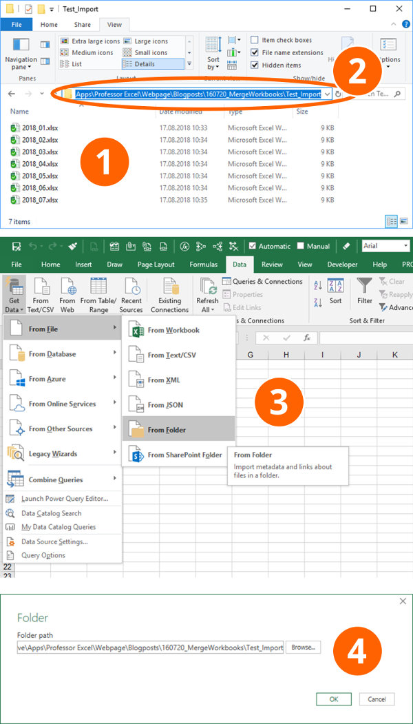
In this example, I want to import all the Excel files from the folder shown below.
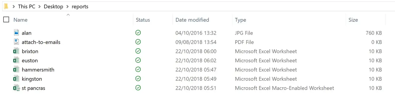
Ideally this folder would contain Excel files ONLY. But when you have teams of people working on a shared area, things happen.
Somehow a PDF file and a JPG (picture of me) have appeared in the folder.
This can create complications with the query we will create to import the Excel files. So we will build in some protection so that the process works seamlessly. Both for now, but also for future imports.
In the future, it will be a case of clicking the Refresh button. And any changed files, or additional files will all be imported again without complication.
Watch the Video
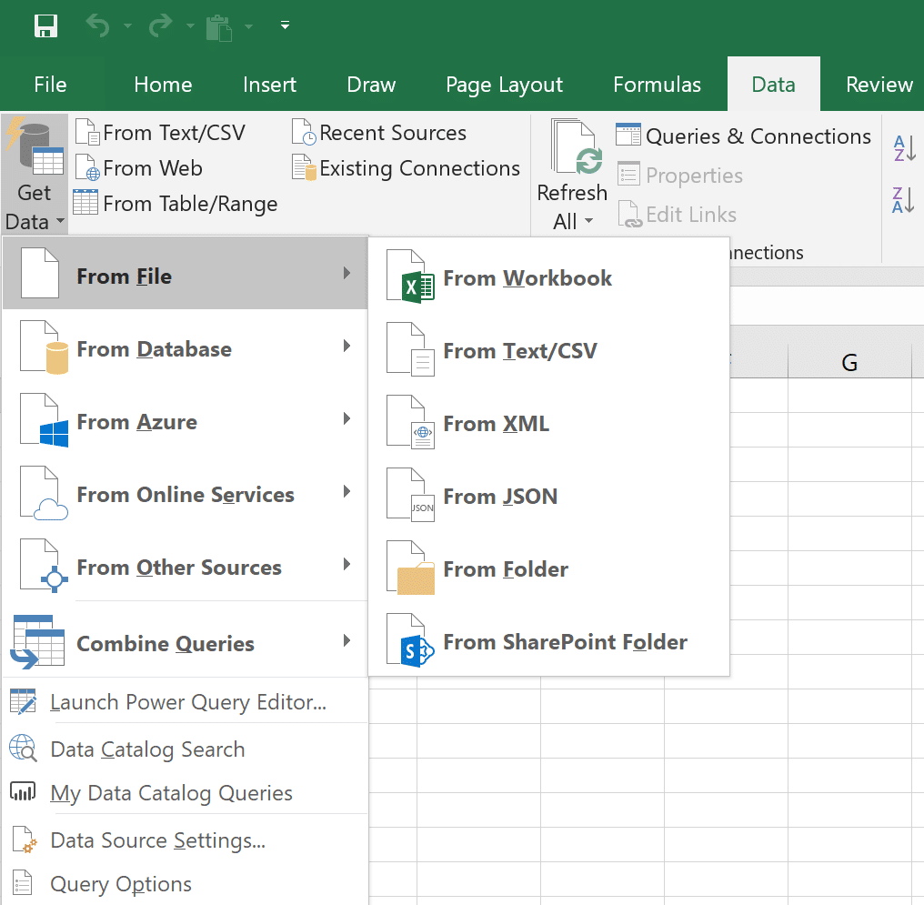
We begin the process by clicking the Data tab > Get Data button > From File and then From Folder.
With the regular changes made to Excel, your screen may look slightly different to above.
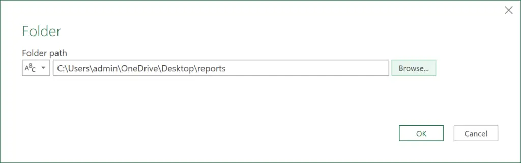
We will then be asked to browse for the folder to import from. I have selected the reports folder on my Desktop.
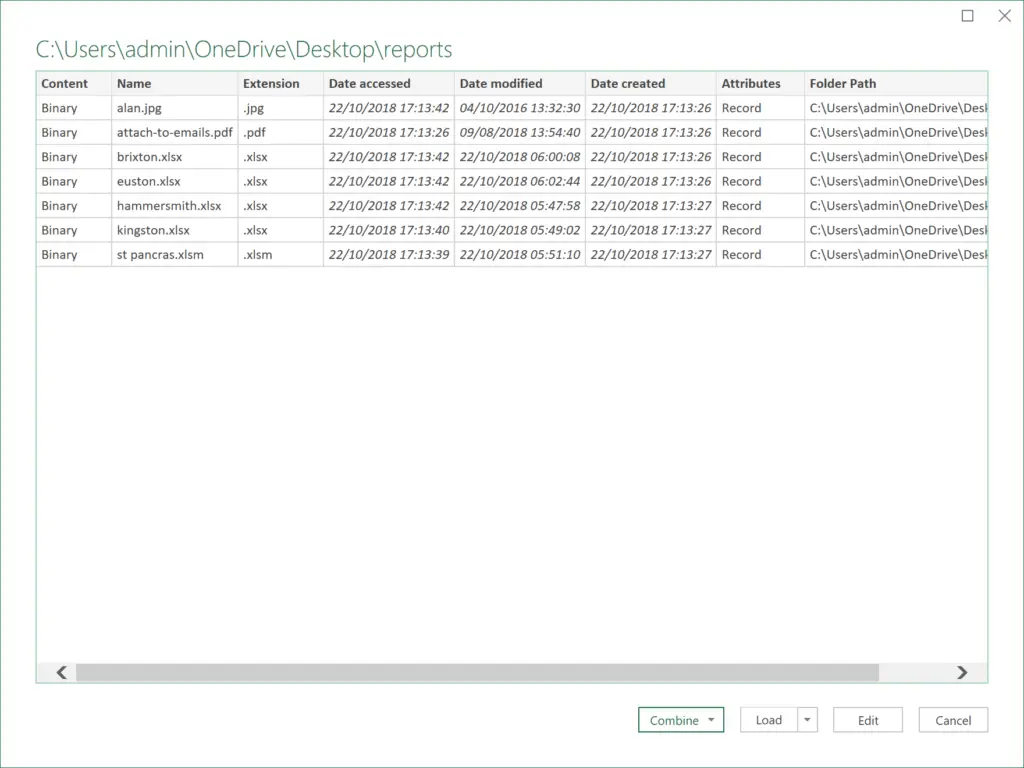
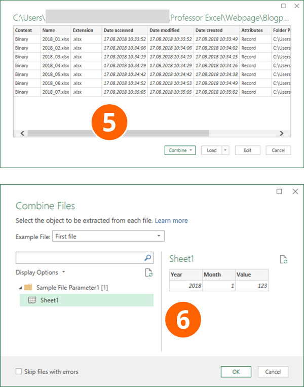
A preview window appears showing the files from that folder.
Click Edit to go to the Power Query Editor. We can then make some changes in here to ensure that only the Excel files are imported.
The files are listed in the editor.
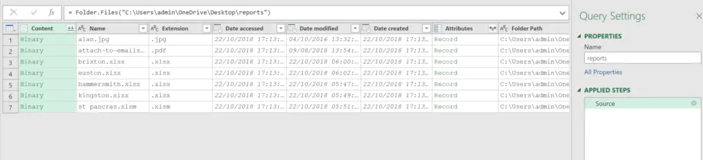
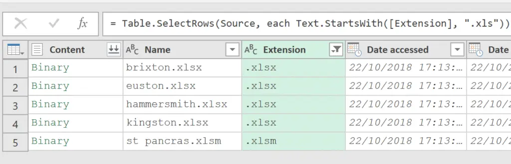
A column with the Extension is provided. This is useful for us to exclude the non Excel files.
Click the filter arrow for the Extension column, select Text Filters and Begins With.
We can then enter .xls to ensure only Excel files are used. This folder also includes a .xlsm (macro enabled worksheet). So by using .xls instead of .xlsx we are catering for .xls, .xlsm and .xlsx files.
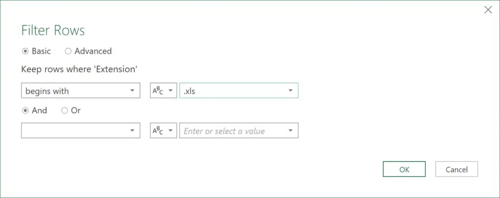
The PDF and JPG files are filtered out of the list. We can now combine the files and append the data from each one into one Excel file.
Click the Combine Files button (double arrow on the Content column header).
The Combine Files window appears. You will see the sheets of the workbooks here and can preview them. Sheet1 is selected as the sheet that includes the data that we want.
The Skip files with errors box has been checked also. This is important to avoid possible errors affecting the import process.
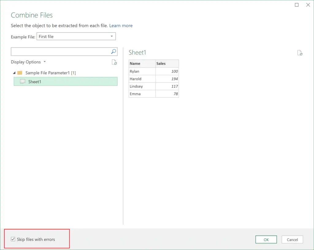
A common error occurs when you try and refresh a connection, but someone has one of the Excel files from that folder open. If you do not check the box to skip errors, your query is interrupted with an error message.
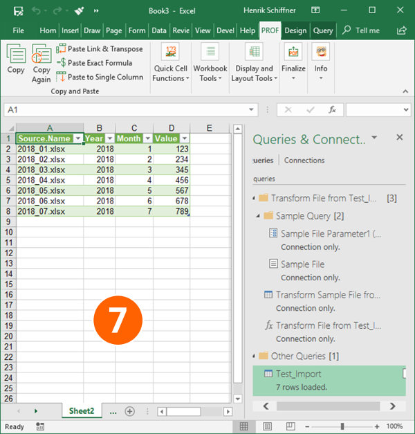
The data from the files is stacked on top of each other into a single list.
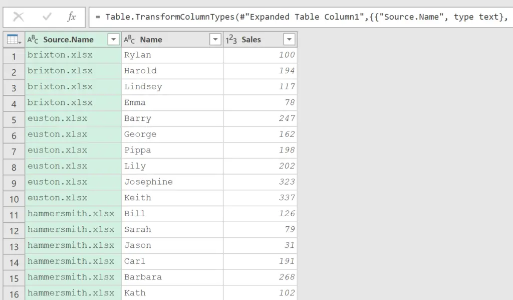
A few more transformations can be done here to make your data look correct.
In the video I split the Source.Name column to separate the extension from the file name. The extension column is then removed. The names converted to capitalise each word. And the column renamed Location to end up with the below.
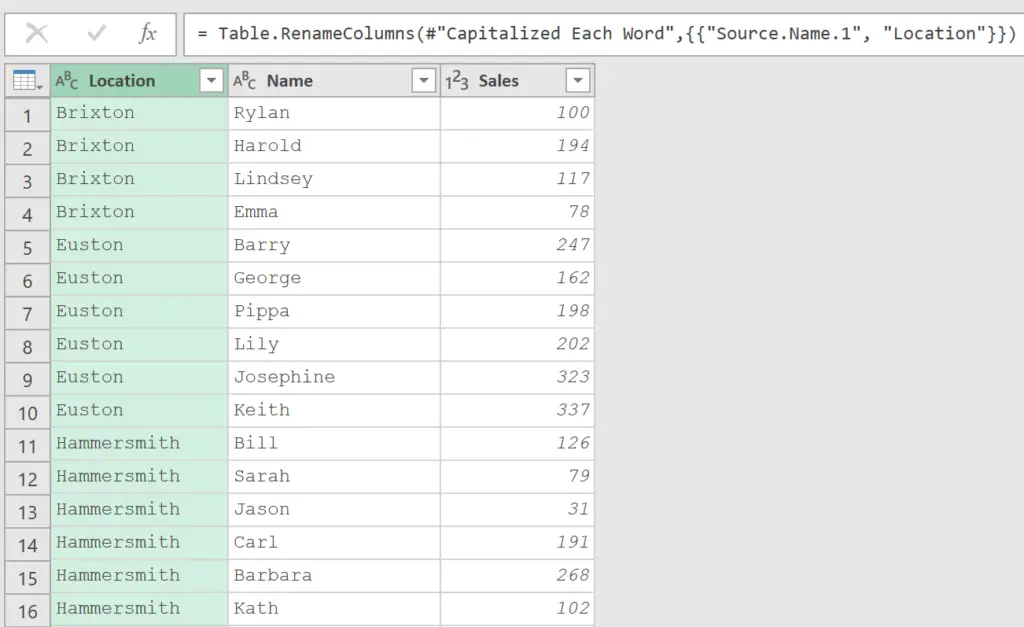
You can then Close and Load the data into a new or existing workbook.
When new files are added, or data changed in those files. You just need to click the Data tab and Refresh to update the connection to that folder, and everything updates.
Superb!
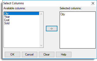
| Select columns for inclusion |
After you click OK this opens a new dialog that lets you select which columns to include in your final spreadsheet.
|
| Sort factor levels | If your data contains factor columns this option will sort the numeric levels (or text labels) into ascending order. |
| Suggest columns to be factors | Genstat will prompt you to convert columns to factors when the column contains x number of repeated values. You can set the number of repeated values in Tools | Spreadsheet Options then click the Conversions tab. Select Suggest converting columns with <=x unique items to factors and set the number as required. |
| Remove empty rows | Remove any rows that contain no data. |
| Remove empty columns | By default, any columns that do not contain data are removed from the Genstat spreadsheet. However, you can keep the empty columns by deselecting this option. |
| Data contains variates & factors only | Any column containing text will be converted to either a variate or factor. If the column contains less than 20% text cells, the column will be made into a variate, otherwise the column will be converted into a factor. |
| Skip first x non-empty rows | The first specified number of rows will be excluded from the spreadsheet. This is useful to exclude any comments that made have been made in the worksheets. Text in these rows can still be used for column names or descriptions – see next option below. |
| Read columns names from file | Controls whether the imported column names are used. Yes if all labels – Read the column names from the row specified in the Column names in row option if all the cells in this row contain labels only or are empty. A default column name will be generated for an empty cell. Yes – Use the cells specified in the Column names in row option . If a cell contains a number, then it will be prefixed with “_” to ensure it is a valid Genstat identifier name. No – Generate default names for the columns, ignoring those in the file. |
| Column names in row | Specifies the row number to use for column names. |
| Column descriptions in row | When selected, the cells in the specified row number will be used for column descriptions. |
| Row numbers (above) are | Controls whether the row numbers are relative to the data range or relate to a whole worksheet. Relative – Row numbers start from the top of the restricted cell range. Absolute – Row numbers start from the top of the worksheet and thus correspond to the absolute row numbering in Excel/Quattro. |
| Text to number | Sometimes numbers are accidentally mistyped as letters. Common mistypings include i, I, l, L for the number 1; o, O for the number 0; a comma for a decimal point, etc. Text to number allows Genstat to convert text labels by substituting numbers for letters or, where this is not possible, the label is converted to a missing value. Strict – Change text strings to numbers only when there are no non-numeric characters in the string. For example, the text ’23’ is converted to 23, the text ‘1a’ contains an alphabetic character so the whole label is converted to a missing value. 1 substitution – Allow a single number to be mistyped and substitute this with the appropriate number. A single lower case ‘o’ or upper case ‘O’ is converted to 0: lower case ‘i’, upper case ‘I’, lower case ‘l’, or upper case ‘L’ is converted to 1. Lower case ‘s’ or upper case ‘S’ is converted to 2. A comma is converted to a decimal point. For example, ‘1o’ contains a single alphabetic character so is converted to 10, ‘1,i’ contains two a comma and an alphabetic characters so is converted to a missing value. Common substitutions – Allows multiple numbers to be mistyped and converts them to the appropriate numbers. For example, ‘LOO’ is converted to 100. Standard – The same as Common substitutions, but any letters at the end of a number are ignored. For example, ’23o’ is converted to 23, ‘i20’ has an alphabetic character at the front so the whole label is converted to a missing value. Lax – Change all text numbers to actual numbers and remove any non-numeric characters. For example, ‘A23X’ is converted to 23. |
| Restricted cell range | Lets you specify a range of cells to import from the worksheet. Type the start and finish cells names separated by a colon, e.g. C1:D96. |
| Add to book | Any open spreadsheets will be displayed in this dropdown list. Select a spreadsheet to insert your data into or leave it at the default setting New Book to create a new workbook. |
| Missing value text | This lets you supply your own text to be inserted into empty cells (the default values are an asterisk * for a variate column or a blank cell for factors and texts). For example, you could use N/A to represent a missing value. |
| Match columns by | Controls how columns are matched between worksheets. Position – matches the worksheet columns by their position i.e. column one in the second worksheet will be appended to column one in the first worksheet, etc. Name – matches and appends worksheet columns that have the same name, regardless of their position. |
| Check for date values | If selected, Genstat checks all text columns to see if they contain data in date format. If any columns appear to contain dates you will be to prompted to convert these to a date format. |
| Set as active sheet |
This sets the new spreadsheet that is created as the active spreadsheet. Setting an active spreadsheet provides a method of avoiding multiple data updates to the server when more than one spreadsheet is open within Genstat. When a spreadsheet is set as the active spreadsheet only data from that spreadsheet is automatically updated to the Genstat server. Another advantage of specifying an active spreadsheet is that the Spread menu options will always be enabled even if your spreadsheet does not have the cursor focus. |
| Ignore case on matching factor labels | If selected, Genstat will match the existing and appended labels even if they use different case e.g. AB and ab will be recognized as the same label. |
You have several Excel workbooks and you want to merge them into one file? This could be a troublesome and long process. But there are 6 different methods of how to merge existing workbooks and worksheets into one file. Depending on the size and number of workbooks, at least one of these methods should be helpful for you. Let’s take a look at them.
Summary
If you want to merge just a small amount of files, go with methods 1 or method 2 below. For anything else, please take a look at the methods 4 to 6: Either use a VBA macro, conveniently use an Excel-add-in or use PowerQuery (PowerQuery only possible if the sheets to merge have exactly the same structure).
Method 1: Copy the cell ranges
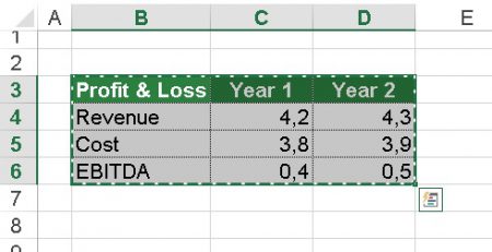
The obvious method: Select the source cell range, copy and paste them into your main workbook. The disadvantage: This method is very troublesome if you have to deal with several worksheets or cell ranges. On the other hand: For just a few ranges it’s probably the fastest way.
Method 2: Manually copy worksheets
The next method is to copy or move one or several Excel sheets manually to another file. Therefore, open both Excel workbooks: The file containing the worksheets which you want to merge (the source workbook) and the new one, which should comprise all the worksheets from the separate files.
- Select the worksheets in your source workbooks which you want to copy. If there are several sheets within one file, hold the Ctrl key
 and click on each sheet tab. Alternatively, go to the first worksheet you want to copy, hold the Shift key
  and click on the last worksheet. That way, all worksheets in between will be selected as well.
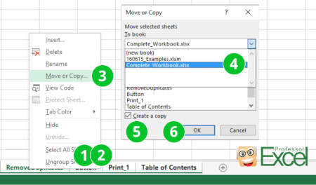
 - Once all worksheets are selected, right click on any of the selected worksheets.
- Click on “Move or Copy”.
- Select the target workbook.
- Set the tick at “Create a copy”. That way, the original worksheets remain in the original workbook and a copy will be created.
- Confirm with OK.

One small tip at this point: You can just drag and drop worksheets from one to another Excel file. Even better: If you press and hold the Ctrl-Key when you drag and drop the worksheets, you create copies.
Do you want to boost your productivity in Excel?
Get the Professor Excel ribbon!

Add more than 120 great features to Excel!
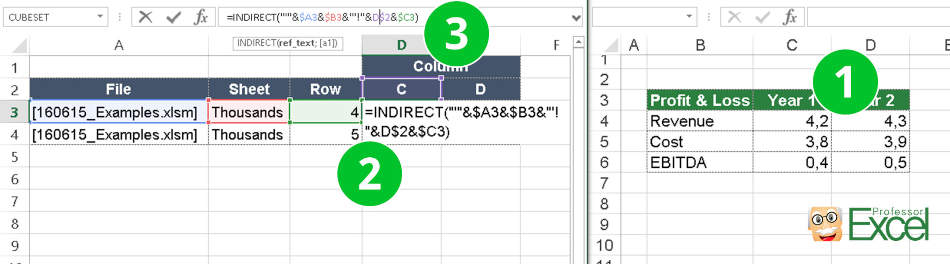
Method 3: Use the INDIRECT formula
The next method comes with some disadvantages and is a little bit more complicated. It works, if your files are in a systematic file order and just want to import some certain values. You build your file and cell reference with the INDIRECT formula. That way, the original files remain and the INDIRECT formula only looks up the values within these files. If you delete the files, you’ll receive #REF! errors.
Let’s take a closer look at how to build the formula. The INDIRECT formula has only one argument: The link to another cell which can also be located within another workbook.
- Copy the first source cell.
- Paste it into your main file using paste special (Ctrl + Alt + v ). Instead of pasting it normally, click on “Link” in the bottom left corner of the Paste Special window. That way, you extract the complete path. In our case, we have the following link:
=[160615_Examples.xlsm]Thousands!$C$4 - Now we wrap the INDIRECT formula around this path. Furthermore, we separate it into file name, sheet name and cell reference. That way, we can later on just change one of these references, for instance for different versions of the same file. The complete formula looks like this (please also see the image above):
=INDIRECT(“‘”&$A3&$B3&”‘!”&D$2&$C3)
Important – please note: This function only works if the source workbooks are open.
Method 4: Merge files with a simple VBA macro
You are not afraid of using a simple VBA macro? Then let’s insert a new VBA module:
- Go to the Developer ribbon. If you can’t see the Developer ribbon, right click on any ribbon and then click on “Customize the Ribbon…”. On the right hand side, set the tick at “Developer”.
- Click on Visual Basic on the left side of the Developer ribbon.
- Right click on your workbook name and click on Insert –> Module.
- Copy and paste the following code into the new VBA module. Position the cursor within the code and click start (the green triangle) on the top. That’s it!
Sub mergeFiles()
    'Merges all files in a folder to a main file.

    'Define variables:
    Dim numberOfFilesChosen, i As Integer
    Dim tempFileDialog As fileDialog
    Dim mainWorkbook, sourceWorkbook As Workbook
    Dim tempWorkSheet As Worksheet

    Set mainWorkbook = Application.ActiveWorkbook
    Set tempFileDialog = Application.fileDialog(msoFileDialogFilePicker)

    'Allow the user to select multiple workbooks
    tempFileDialog.AllowMultiSelect = True

    numberOfFilesChosen = tempFileDialog.Show

    'Loop through all selected workbooks
    For i = 1 To tempFileDialog.SelectedItems.Count

        'Open each workbook
        Workbooks.Open tempFileDialog.SelectedItems(i)

        Set sourceWorkbook = ActiveWorkbook

        'Copy each worksheet to the end of the main workbook
        For Each tempWorkSheet In sourceWorkbook.Worksheets
            tempWorkSheet.Copy after:=mainWorkbook.Sheets(mainWorkbook.Worksheets.Count)
        Next tempWorkSheet

        'Close the source workbook
        sourceWorkbook.Close
    Next i

End Sub
Method 5: Automatically merge workbooks
The fifth way is probably most convenient:
Click on “Merge Files” on the Professor Excel ribbon.
Now select all the files and worksheets you want to merge and start with “OK”.
This procedure works well also for many files at the same time and is self-explanatory. Even better: Besides XLSX files, you can also combine XLS, XLSB, XLSM, CSV, TXT and ODS files.
To do that you need a third party add-in, for example our popular “Professor Excel Tools” (click here to start the download).
Here is the whole process in detail:
Method 6: Use the Get & Transform tools (PowerQuery)
The current version of Excel 365 offers the “Get & Transform” tools to import data. These functions are very powerful and are supposed to replace the old “Text Import Wizard”. However, they have one useful feature: Import a complete folder of documents.
The requirements: The workbooks and worksheets you want to import have to be in the same format.
Please follow these steps for importing a complete folder of Excel files.
- Create a folder with all the documents you want to import.
- Usually it’s the fastest to just copy the folder path directly from the Windows Explorer. You still have the change to later-on select the folder, though.
- Within Excel, go to the Data ribbon and click on “Get Data”, “From File” and then on “From Folder”.
- Paste the previously copied path or select it via the “Browse” function. Continue with “OK”.
- If all files are shown in the following window, either click on “Combine” (and then on “Combine & Load To”) or on “Edit”. If you click on “Edit”, you can still filter the list and only import a selection of the files in the list. Recommendation: Put only the necessary files into your import folder from the beginning so that you don’t have to navigate through the complex “Edit” process.
- Next, Excel shows an example of the data based on the first file. If everything seems fine, click on OK. If your files have several sheets, just select the one you want to import, in this example “Sheet1”. Click on “OK”.
- That’s it, Excel now imports the data and inserts a new column containing the file name.
For more information about the Get & Transform tools please refer to this article.
Next step: Merge multiple worksheets to one combined sheet
After you have combined many Excel workbooks into one file, usually the next step is this: Merge all the imported sheets into one worksheet.
Because this is a whole different topic by itself, please refer to this article.
Image by MartinHolzer from Pixabay
You have several Excel files that make it harder for you to access data. You keep switching between different opened files, and this process takes a lot of your time. You are well aware that it is a lot easier to process data in a single file instead of switching between numerous sources. Then comes the question, how can I merge all these files into one comprehensive file? It is a troublesome and long process trying to combine different Excel files into one file when you factor in the number of worksheets found in one workbook. There are various ways of merging Excel files.
In this article, we discuss how to merge multiple Excel files into one file. Let’s get started.
Method 1: Combine multiple workbooks into one workbook with the Move or Copy function
1. If you want to merge all the existing files into a new Excel workbook, create the new Excel workbook and open it. But if you’re going to combine all of them into a current workbook, open that workbook.


2. Open all the Excel files you want to merge. You need to open all files to be able to combine them into one. Instead of doing it manually, select all the files and press the enter key on your keyboard. To select multiple files that are non-adjacent, hold the Ctrl key and click the files one by one. For adjacent files, hold the Shift key and click on the last file to select them all.

3. Maximize the first file you want to merge.
4. Right-click the worksheet you want to merge, then select Move or Copy.

5. On the pop-up window, click ‘Pick from Drop-down List.’ All the Excel files opened on your computer will be displayed here

6. Select the excel file you want to merge other files into in the ‘To book’ drop-down arrow.

7. To merge excel files, check the Create a copy checkbox.

8. In the Before Sheet section, select ‘move to end and click OK. It will create a copy of the worksheet in the destination file.

9. Repeat all the above steps for all the remaining files and save your file.
Method 2: Combine multiple workbooks into one with VBA
1. Open a new workbook that will act as a master workbook.

2. Press Alt + F11 to the VBA page

3. Click on the Insert tab. Next, select the Module tab.

4. Copy and paste the macro code below.
Sub GetSheets()
Path = "C:UsersdtDesktopdt kte"
Filename = Dir(Path & "*.xlsx")
Do While Filename <> ""
Workbooks.Open Filename:=Path & Filename, ReadOnly:=True
For Each Sheet In ActiveWorkbook.Sheets
Sheet.Copy After:=ThisWorkbook.Sheets(1)
Next Sheet
Workbooks(Filename).Close
Filename = Dir()
Loop
End Sub
Click here for more code.
5. After this, it is time to initiate the command by pressing F5 to run the excel macro code. Doing this will open a file and then copy the data. It will paste the same in your new workbook. Close the workbook.

Method 3: Merging Microsoft Excel files as CSV files.
1. Open the excel files.
2. Go to the Menu bar. Click File. Then Save As.
4. In the Save as type, there is a drop-down list. Select CSV from the list.

5. Do this for all the files you want to merge, and then place all the CSV files into one folder.

6. Open the command prompt then navigate to your folder. Type the following command to merge all CSV files in the folder into a new CSV file. Copy *.csv newfile.CSV

7. After creating the new file, open the new CSV file in Microsoft Excel.
8. Save it as an Excel file.

Method 4: Using Power Query
The Power Query method is the best way to merge data since you only need to store all the excel files in a single folder. You can then use that folder to load data from files into the Power Query Editor. It also allows you to transform data while combining.
However, for the Power Query editor to merge Excel files, you need to understand that all data should be structured in the same way. That means the number of columns and their order should be the same. Below are steps to follow when merging files with the Power Query application.
Power query allows to import, edit and consolidate the data. It can also be used to import and combine multiple excel files into one folder.
With the Same Name of Worksheets and Tables
1. Move all the files into the new folder that you want to combine.

2. In Excel go to the Data tab

3. Press Get Dat > From File > From Folder

4. Browse and select the folder path

5. Press Ok
6. If files are ready to combine press Combine & Load

7. If you want to manipulate the data, then press the Transform Data button. This will open the query editor where you can work on the data.

From here, select the table in which you have data in all the workbooks. A preview of this will appear at the side of the window.

8. Once you select the table, click OK to merge data from all the files into your Power Query editor. You will see a new column with the name of the workbooks from which data is extracted.

9. Right-click on the column header and select “Replace Values”.

10. Enter the text “.xlsx” in the Replace Values box and leave the “Replace With” box blank. The idea here is to remove the file extension from the name of the workbook.

11. Next, double-click on the header and select “Rename” to enter a name for the column.

12. At this point, your merged data is ready and you only need to load it into your new workbook. To perform this, go to the Home Tab and click on Close & Load. Now you will have your combined data from all tables or workbooks with the same name in a single workbook.

Note: You will not have the same table name in all the excel files all the time. At that point, you can use the worksheet name to combine data with the Power Query method. However, you should note two points when using the worksheet name to combine data with the power query method:
- Power Query is case-sensitive. So, you should have the same letter names of worksheets in all the workbooks.
- You should have the same name for the column headers, but the order of the columns does not matter. If column1 in the north.xlxs is column2 in the west.xlxs, Power Query will match it, but you need to have the same column names.
Therefore, when combining files using the power query, you can use the worksheet name instead of the table name. You only need to select the worksheet name, click on the Combine & Edit, and follow all the steps outlined above from step number 6.
When You Don’t Have the Same Name of Worksheets and Tables.
In some situations, you can lack the same name of worksheets and tables in the excel files. In this case, you must know how to combine data from these different worksheets and tables into one file, following these steps:
1. Open the “From Folder” dialog box to locate the folder where you have all the files and click OK.

2. After that, click on the “Edit” to edit the table.
3. Once the table and Power Query editor open, select the first two columns of the table and click on the Remove other Columns from the right-click menu.

4. From here, you need to add a custom column to fetch data from the worksheets of the workbooks. To do this, go to Add Column Tab and click on the Custom Column button. The step will automatically open the Custom Column in the dialog box.

5. In the dialog box enter the formula below and click OK.
=Excel.Workbook([Content])

6. You will have a new column in the table from which you need to extract data. Open the filter from that newly added custom column and click OK to expand all the data into the table.
7. You will see a newly expanded table with some new columns. Delete all columns from the new table except the third and the fourth column.

8. Now open the filter for the Custom Data column to expand it and click OK.

Once you click OK, you will get all the data from the files having been merged into a single table. Though, if you notice all the headings of the columns are in the data itself, you need to add the column headings as follows;
- Double-click on the header and add a name. You can also right-click and select Rename It.
- Exclude the headings you have in the data table. For this, open any column’s filter options and unselect the heading name which you have in the column data and click OK after that. After you click ok, your data is ready to load into the worksheet.
- Go to the Home Tab and click on Close and Load. This allows you to combine data from different workbooks that had different worksheets names.

At this point, you have already merged the data into one single file. You should then apply some formatting to avoid losing a single file of your data when updating it. To format a single file, you can use these steps:
- Go to Design Tab and open Properties.
- Untick the Adjust Column width and tick the Preserve Cell Formatting
Conclusion
The above tips help you to be organized and save time. Whether you decide to merge data in excel into a single file, or if you prefer to spread your work across multiple files, either of the methods above will help you. Excel offers immense features such as an in-built tracking feature that keeps track of any changes made in your files. So, losing your original data should not be a cause of dilemma.
You can use Object Linking and Embedding (OLE) to include content from other programs, such as Word or Excel.
OLE is supported by many different programs, and OLE is used to make content that is created in one program available in another program. For example, you can insert an Office Word document in an Office Excel workbook. To see what types of content that you can insert, click Object in the Text group on the Insert tab. Only programs that are installed on your computer and that support OLE objects appear in the Object type box.
If you copy information between Excel or any program that supports OLE, such as Word, you can copy the information as either a linked object or an embedded object. The main differences between linked objects and embedded objects are where the data is stored and how the object is updated after you place it in the destination file. Embedded objects are stored in the workbook that they are inserted in, and they are not updated. Linked objects remain as separate files, and they can be updated.
Linked and embedded objects in a document
1. An embedded object has no connection to the source file.
2. A linked object is linked to the source file.
3. The source file updates the linked object.
When to use linked objects
If you want the information in your destination file to be updated when the data in the source file changes, use linked objects.
With a linked object, the original information remains stored in the source file. The destination file displays a representation of the linked information but stores only the location of the original data (and the size if the object is an Excel chart object). The source file must remain available on your computer or network to maintain the link to the original data.
The linked information can be updated automatically if you change the original data in the source file. For example, if you select a paragraph in a Word document and then paste the paragraph as a linked object in an Excel workbook, the information can be updated in Excel if you change the information in your Word document.
When to use embedded objects
If you don’t want to update the copied data when it changes in the source file, use an embedded object. The version of the source is embedded entirely in the workbook. If you copy information as an embedded object, the destination file requires more disk space than if you link the information.
When a user opens the file on another computer, he can view the embedded object without having access to the original data. Because an embedded object has no links to the source file, the object is not updated if you change the original data. To change an embedded object, double-click the object to open and edit it in the source program. The source program (or another program capable of editing the object) must be installed on your computer.
Changing the way that an OLE object is displayed
You can display a linked object or embedded object in a workbook exactly as it appears in the source program or as an icon. If the workbook will be viewed online, and you don’t intend to print the workbook, you can display the object as an icon. This minimizes the amount of display space that the object occupies. Viewers who want to display the information can double-click the icon.
Embed an object in a worksheet
-
Click inside the cell of the spreadsheet where you want to insert the object.
-
On the Insert tab, in the Text group, click Object
 .
. -
In the Object dialog box, click the Create from File tab.
-
Click Browse, and select the file you want to insert.
-
If you want to insert an icon into the spreadsheet instead of show the contents of the file, select the Display as icon check box. If you don’t select any check boxes, Excel shows the first page of the file. In both cases, the complete file opens with a double click. Click OK.
Note: After you add the icon or file, you can drag and drop it anywhere on the worksheet. You can also resize the icon or file by using the resizing handles. To find the handles, click the file or icon one time.
 .
.
Insert a link to a file
You might want to just add a link to the object rather than fully embedding it. You can do that if your workbook and the object you want to add are both stored on a SharePoint site, a shared network drive, or a similar location, and if the location of the files will remain the same. This is handy if the linked object undergoes changes because the link always opens the most up-to-date document.
Note: If you move the linked file to another location, the link won’t work anymore.
-
Click inside the cell of the spreadsheet where you want to insert the object.
-
On the Insert tab, in the Text group, click Object
. -
Click the Create from File tab.
-
Click Browse, and then select the file you want to link.
-
Select the Link to file check box, and click OK.
Create a new object from inside Excel
You can create an entirely new object based on another program without leaving your workbook. For example, if you want to add a more detailed explanation to your chart or table, you can create an embedded document, such as a Word or PowerPoint file, in Excel. You can either set your object to be displayed right in a worksheet or add an icon that opens the file.

-
Click inside the cell of the spreadsheet where you want to insert the object.
-
On the Insert tab, in the Text group, click Object
. -
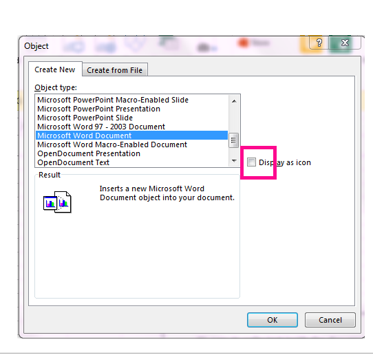
On the Create New tab, select the type of object you want to insert from the list presented. If you want to insert an icon into the spreadsheet instead of the object itself, select the Display as icon check box.
-
Click OK. Depending on the type of file you are inserting, either a new program window opens or an editing window appears within Excel.
-
Create the new object you want to insert.
When you’re done, if Excel opened a new program window in which you created the object, you can work directly within it.
When you’re done with your work in the window, you can do other tasks without saving the embedded object. When you close the workbook your new objects will be saved automatically.
Note: After you add the object, you can drag and drop it anywhere on your Excel worksheet. You can also resize the object by using the resizing handles. To find the handles, click the object one time.

Embed an object in a worksheet
-
Click inside the cell of the spreadsheet where you want to insert the object.
-
On the Insert tab, in the Text group, click Object.
-
Click the Create from File tab.
-
Click Browse, and select the file you want to insert.
-
If you want to insert an icon into the spreadsheet instead of show the contents of the file, select the Display as icon check box. If you don’t select any check boxes, Excel shows the first page of the file. In both cases, the complete file opens with a double click. Click OK.
Note: After you add the icon or file, you can drag and drop it anywhere on the worksheet. You can also resize the icon or file by using the resizing handles. To find the handles, click the file or icon one time.
Insert a link to a file
You might want to just add a link to the object rather than fully embedding it. You can do that if your workbook and the object you want to add are both stored on a SharePoint site, a shared network drive, or a similar location, and if the location of the files will remain the same. This is handy if the linked object undergoes changes because the link always opens the most up-to-date document.
Note: If you move the linked file to another location, the link won’t work anymore.
-
Click inside the cell of the spreadsheet where you want to insert the object.
-
On the Insert tab, in the Text group, click Object.
-
Click the Create from File tab.
-
Click Browse, and then select the file you want to link.
-
Select the Link to file check box, and click OK.
Create a new object from inside Excel
You can create an entirely new object based on another program without leaving your workbook. For example, if you want to add a more detailed explanation to your chart or table, you can create an embedded document, such as a Word or PowerPoint file, in Excel. You can either set your object to be displayed right in a worksheet or add an icon that opens the file.
-
Click inside the cell of the spreadsheet where you want to insert the object.
-
On the Insert tab, in the Text group, click Object.
-
On the Create New tab, select the type of object you want to insert from the list presented. If you want to insert an icon into the spreadsheet instead of the object itself, select the Display as icon check box.
-
Click OK. Depending on the type of file you are inserting, either a new program window opens or an editing window appears within Excel.
-
Create the new object you want to insert.
When you’re done, if Excel opened a new program window in which you created the object, you can work directly within it.
When you’re done with your work in the window, you can do other tasks without saving the embedded object. When you close the workbook your new objects will be saved automatically.
Note: After you add the object, you can drag and drop it anywhere on your Excel worksheet. You can also resize the object by using the resizing handles. To find the handles, click the object one time.
Link or embed content from another program by using OLE
You can link or embed all or part of the content from another program.
Create a link to content from another program
-
Click in the worksheet where you want to place the linked object.
-
On the Insert tab, in the Text group, click Object.
-
Click the Create from File tab.
-
In the File name box, type the name of the file, or click Browse to select from a list.
-
Select the Link to file check box.
-
Do one of the following:
-
To display the content, clear the Display as icon check box.
-
To display an icon, select the Display as icon check box. Optionally, to change the default icon image or label, click Change Icon, and then click the icon that you want from the Icon list, or type a label in the Caption box.
Note: You cannot use the Object command to insert graphics and certain types of files. To insert a graphic or file, on the Insert tab, in the Illustrations group, click Picture.
-
Embed content from another program
-
Click in the worksheet where you want to place the embedded object.
-
On the Insert tab, in the Text group, click Object.
-
If the document does not already exist, click the Create New tab. In the Object type box, click the type of object that you want to create.
If the document already exists, click the Create from File tab. In the File name box, type the name of the file, or click Browse to select from a list.
-
Clear the Link to file check box.
-
Do one of the following:
-
To display the content, clear the Display as icon check box.
-
To display an icon, select the Display as icon check box. To change the default icon image or label, click Change Icon, and then click the icon that you want from the Icon list, or type a label in the Caption box.
-
Link or embed partial content from another program
-
From a program other than Excel, select the information that you want to copy as a linked or embedded object.
-
On the Home tab, in the Clipboard group, click Copy.
-
Switch to the worksheet that you want to place the information in, and then click where you want the information to appear.
-
On the Home tab, in the Clipboard group, click the arrow below Paste, and then click Paste Special.
-
Do one of the following:
-
To paste the information as a linked object, click Paste link.
-
To paste the information as an embedded object, click Paste. In the As box, click the entry with the word «object» in its name. For example, if you copied the information from a Word document, click Microsoft Word Document Object.
-

Change the way that an OLE object is displayed
-
Right-click the icon or object, point to object typeObject (for example, Document Object), and then click Convert.
-
Do one of the following:
-
To display the content, clear the Display as icon check box.
-
To display an icon, select the Display as icon check box. Optionally, you can change the default icon image or label. To do that, click Change Icon, and then click the icon that you want from the Icon list, or type a label in the Caption box.
-
Control updates to linked objects
You can set links to other programs to be updated in the following ways: automatically, when you open the destination file; manually, when you want to see the previous data before updating with the new data from the source file; or when you specifically request the update, regardless of whether automatic or manual updating is turned on.
Set a link to another program to be updated manually
-
On the Data tab, in the Connections group, click Edit Links.
Note: The Edit Links command is unavailable if your file does not contain links to other files.
-
In the Source list, click the linked object that you want to update. An A in the Update column means that the link is automatic, and an M in the Update column means that the link is set to Manual update.
Tip: To select multiple linked objects, hold down CTRL and click each linked object. To select all linked objects, press CTRL+A.
-
To update a linked object only when you click Update Values, click Manual.
Set a link to another program to be updated automatically
-
On the Data tab, in the Connections group, click Edit Links.
Note: The Edit Links command is unavailable if your file does not contain links to other files.
-
In the Source list, click the linked object that you want to update. An A in the Update column means that the link will update automatically, and an M in the Update column means that the link must be updated manually.
Tip: To select multiple linked objects, hold down CTRL and click each linked object. To select all linked objects, press CTRL+A.
-
Click OK.
Issue: I can’t update the automatic links on my worksheet
The Automatic option can be overridden by the Update links to other documents Excel option.
To ensure that automatic links to OLE objects can be automatically updated:
-
Click the Microsoft Office Button
, click Excel Options, and then click the Advanced category. -
Under When calculating this workbook, make sure that the Update links to other documents check box is selected.
 , click Excel Options, and then click the Advanced category.
Update a link to another program now
-
On the Data tab, in the Connections group, click Edit Links.
Note: The Edit Links command is unavailable if your file does not contain linked information.
-
In the Source list, click the linked object that you want to update.
Tip: To select multiple linked objects, hold down CTRL and click each linked object. To select all linked objects, press CTRL+A.
-
Click Update Values.
Edit content from an OLE program
While you are in Excel, you can change the content linked or embedded from another program.
Edit a linked object in the source program
-
On the Data tab, in the Connections group, click Edit Links.
Note: The Edit Links command is unavailable if your file does not contain linked information.
-
In the Source file list, click the source for the linked object, and then click Open Source.
-
Make the changes that you want to the linked object.
-
Exit the source program to return to the destination file.
Edit an embedded object in the source program
-
Double-click the embedded object to open it.
-
Make the changes that you want to the object.
-
If you are editing the object in place within the open program, click anywhere outside of the object to return to the destination file.
If you edit the embedded object in the source program in a separate window, exit the source program to return to the destination file.
Note: Double-clicking certain embedded objects, such as video and sound clips, plays the object instead of opening a program. To edit one of these embedded objects, right-click the icon or object, point to object typeObject (for example, Media Clip Object), and then click Edit.
Edit an embedded object in a program other than the source program
-
Select the embedded object that you want to edit.
-
Right-click the icon or object, point to object typeObject (for example, Document Object), and then click Convert.
-
Do one of the following:
-
To convert the embedded object to the type that you specify in the list, click Convert to.
-
To open the embedded object as the type that you specify in the list without changing the embedded object type, click Activate.
-
Select an OLE object by using the keyboard
-
Press CTRL+G to display the Go To dialog box.
-
Click Special, select Objects, and then click OK.
-
Press TAB until the object that you want is selected.
-
Press SHIFT+F10.
-
Point to Object or Chart Object, and then click Edit.
Issue: When I double-click a linked or embedded object, a «cannot edit» message appears
This message appears when the source file or source program can’t be opened.
Make sure that the source program is available If the source program is not installed on your computer, convert the object to the file format of a program that you do have installed.
Ensure that memory is adequate Make sure that you have enough memory to run the source program. Close other programs to free up memory, if necessary.
Close all dialog boxes If the source program is running, make sure that it doesn’t have any open dialog boxes. Switch to the source program, and close any open dialog boxes.
Close the source file If the source file is a linked object, make sure that another user doesn’t have it open.
Ensure that the source file name has not changed If the source file that you want to edit is a linked object, make sure that it has the same name as it did when you created the link and that it has not been moved. Select the linked object, and then click the Edit Links command in the Connections group on the Data tab to see the name of the source file. If the source file has been renamed or moved, use the Change Source button in the Edit Links dialog box to locate the source file and reconnect the link.
Need more help?
You can always ask an expert in the Excel Tech Community or get support in the Answers community.