
Append queries
- To open a query, locate one previously loaded from the Power Query Editor, select a cell in the data, and then select Query > Edit. For more information see Create, load, or edit a query in Excel.
- Select Home > Append Queries.
- Decide the number of tables you want to append:
- Select OK.
Contents
- 1 How do I append in Excel?
- 2 What does it mean to append data in Excel?
- 3 How do I append data from another sheet in Excel?
- 4 How do I append data to a table in Excel?
- 5 How do I append text in Excel?
- 6 How do you append data?
- 7 What is the difference between append and merge?
- 8 How do you use concatenate?
- 9 How do you auto populate data from multiple sheets to a master?
- 10 How do you combine cells in Excel without losing data?
- 11 How do I add a space between words in Excel?
- 12 How do you append data in access without duplicates?
- 13 How do you write an append query?
- 14 What is merge query?
- 15 How do you merge tables?
- 16 How do you CONCATENATE 3 columns in Excel?
- 17 What is the Ifna function in Excel?
- 18 How do I append to a column in Excel?
- 19 How do I auto populate data in Excel based on another cell?
- 20 How do I combine data from multiple sheets on one page in Excel?
Appending text from one cell to another with formula
You can use formula to append text from one cell to another as follows. 1. Select a blank cell for locating the appended result, enter formula =CONCATENATE(A1,” “,B1,” “,C1) into the formula bar, and then press the Enter key.
What does it mean to append data in Excel?
Append means to add to; when you append multiple worksheets, you are adding one worksheet to another. This could mean you are adding a worksheet or multiple worksheets to an existing one, or combining all into one new worksheet. This lesson will introduce you to the Consolidate tool in Excel.
How do I append data from another sheet in Excel?
On the Data tab, under Tools, click Consolidate. In the Function box, click the function that you want Excel to use to consolidate the data. In each source sheet, select your data, and then click Add. The file path is entered in All references.
How do I append data to a table in Excel?
Once the data is selected, click over the table you want to append data to, inside the main panel. Finally, click the Append Excel Data to Table action label when it becomes enabled.
How do I append text in Excel?
Combine text from two or more cells into one cell
- Select the cell where you want to put the combined data.
- Type = and select the first cell you want to combine.
- Type & and use quotation marks with a space enclosed.
- Select the next cell you want to combine and press enter. An example formula might be =A2&” “&B2.
How do you append data?
On the Home tab, in the View group, click View, and then click Design View. On the Design tab, in the Query Type group, click Append. The Append dialog box appears. Next, you specify whether to append records to a table in the current database, or to a table in a different database.
What is the difference between append and merge?
Merge will join two tables horizontally adding columns based on matching key columns like vlookup in Excel from the 2nd table, but append, you add rows from the 2nd or more tables to the 1st table the end.
How do you use concatenate?
There are two ways to do this:
- Add double quotation marks with a space between them ” “. For example: =CONCATENATE(“Hello”, ” “, “World!”).
- Add a space after the Text argument. For example: =CONCATENATE(“Hello “, “World!”). The string “Hello ” has an extra space added.
How do you auto populate data from multiple sheets to a master?
How to collect data from multiple sheets to a master sheet in…
- In a new sheet of the workbook which you want to collect data from sheets, click Data > Consolidate.
- In the Consolidate dialog, do as these: (1 Select one operation you want to do after combine the data in Function drop down list;
- Click OK.
How do you combine cells in Excel without losing data?
How to merge cells in Excel without losing data
- Select all the cells you want to combine.
- Make the column wide enough to fit the contents of all cells.
- On the Home tab, in the Editing group, click Fill > Justify.
- Click Merge and Center or Merge Cells, depending on whether you want the merged text to be centered or not.
How do I add a space between words in Excel?
Select a blank cell, enter formula =AddSpace(B2) into the Formula Bar, then press the Enter key. In this case, you can see spaces are added between characters of cell B2. Note: For adding space between every digits, please change the cell reference in the formula to the one with numbers as you need.
How do you append data in access without duplicates?
In the Append dialog box, select the blank database Customers Without Duplicates, as shown in Figure K. Click the Run button. In the dialog box that asks whether you wish to append the records to the new file, click Yes.
How do you write an append query?
Create an Append Query
- Click the Create tab on the ribbon.
- Click the Query Design button.
- Select the tables and queries you want to add and click Add.
- Click Close.
- Click the Append button.
- Select the Current Database or Another Database option.
- Click the Table Name list arrow and select the table.
- Click the OK.
What is merge query?
A merge query creates a new query from two existing queries. One query result contains all columns from a primary table, with one column serving as a single column containing a relationship to a secondary table. The related table contains all rows that match each row from a primary table based on a common column value.
How do you merge tables?
Method 2: Use “Merge Table” Option
- Firstly, click on the cross sign to select the first table.
- Then press “Ctrl+ X” to cut the table.
- Next place cursor at the start of the line right below the second table.
- And right click.
- Lastly, on the contextual menu, choose “Merge Table”.
How do you CONCATENATE 3 columns in Excel?
How to Combine Three Columns in Excel
- Open your spreadsheet.
- Select the cell where you want to display the combined data.
- Type =CONCATENATE(AA, BB, CC) but insert your cell locations.
- Adjust the formula to include any needed spaces or punctuation.
What is the Ifna function in Excel?
The IFNA function returns the value you specify if a formula returns the #N/A error value; otherwise it returns the result of the formula.
How do I append to a column in Excel?
Append value(s) to a column (before or after)
- Select a single cell in table column you want, then invoke ‘DigDB->Column->Append…’ The column to append will be automatically selected.
- Enter the values you want to append.
- Click ‘OK’ to append.
How do I auto populate data in Excel based on another cell?
Anyone who has used Excel for some time knows how to use the autofill feature to autofill an Excel cell based on another. You simply click and hold your mouse on the lower right corner of the cell, and drag it down to apply the formula in that cell to every cell beneath it (similar to copying formulas in Excel).
How do I combine data from multiple sheets on one page in Excel?
On the Excel ribbon, go to the Ablebits tab, Merge group, click Copy Sheets, and choose one of the following options:
- Copy sheets in each workbook to one sheet and put the resulting sheets to one workbook.
- Merge the identically named sheets to one.
- Copy the selected sheets to one workbook.
Note: Microsoft Access doesn’t support importing Excel data with an applied sensitivity label. As a workaround, you can remove the label before importing and then re-apply the label after importing. For more information, see Apply sensitivity labels to your files and email in Office.
You can bring the data from an Excel workbook into Access databases in many ways. You can copy data from an open worksheet and paste it into an Access datasheet, import a worksheet into a new or existing table, or link to a worksheet from an Access database.
This topic explains in detail how to import or link to Excel data from Access desktop databases.
What do you want to do?
-
Understand importing data from Excel
-
Import data from Excel
-
Troubleshoot missing or incorrect values
-
Link to data in Excel
-
Troubleshoot #Num! and other incorrect values in a linked table
Understand importing data from Excel
If your goal is to store some or all of your data from one or more Excel worksheets in Access, you should import the contents of the worksheet into a new or existing Access database. When you import data, Access creates a copy of the data in a new or existing table without altering the source Excel worksheet.
Common scenarios for importing Excel data into Access
-
You are a long-time user of Excel but, going forward, you want to use Access to work with this data. You want to move the data in your Excel worksheets into one or more new Access databases.
-
Your department or workgroup uses Access, but you occasionally receive data in Excel format that must be merged with your Access databases. You want to import these Excel worksheets into your database as you receive them.
-
You use Access to manage your data, but the weekly reports you receive from the rest of your team are Excel workbooks. You would like to streamline the import process to ensure that data is imported every week at a specific time into your database.
If this is the first time you are importing data from Excel
-
There is no way to save an Excel workbook as an Access database. Excel does not provide functionality to create an Access database from Excel data.
-
When you open an Excel workbook in Access (in the File Open dialog box, change the Files of Type list box to Microsoft Office Excel Files and select the file you want), Access creates a link to the workbook instead of importing its data. Linking to a workbook is fundamentally different from importing a worksheet into a database. For more information about linking, see the section Link to data in Excel, later in this article.
Import data from Excel
The steps in this section explain how to prepare for and run an import operation, and how to save the import settings as a specification for later reuse. As you proceed, remember that you can import data from only one worksheet at a time. You cannot import all the data from a whole workbook at the same time.
Prepare the worksheet
-
Locate the source file and select the worksheet that contains the data that you want to import to Access. If you want to import only a portion of a worksheet, you can define a named range that includes only the cells that you want to import.
Define a named range (optional)
-
Switch to Excel and open the worksheet that has data that you want to import.
-
Select the range of cells that contain the data that you want to import.
-
Right-click within the selected range and then click Name a Range or Define Name.
-
In the New Name dialog box, specify a name for the range in the Name box and click OK.
Remember that you can import only one worksheet at a time during an import operation. To import data from multiple worksheets, repeat the import operation for each worksheet.
-
-
Review the source data and take action as described in this table.
Element
Description
Number of columns
The number of source columns that you want to import cannot exceed 255, because Access does not support more than 255 fields in a table.
Skipping columns and rows
It is a good practice to include only the rows and columns that you want to import in the source worksheet or named range.
Rows You cannot filter or skip rows during the import operation.
Columns You cannot skip columns during the operation if you choose to add the data to an existing table.
Tabular format
Ensure that the cells are in tabular format. If the worksheet or named range includes merged cells, the contents of the cell are placed in the field that corresponds to the leftmost column, and the other fields are left blank.
Blank columns, rows, and cells
Delete all unnecessary blank columns and blank rows in the worksheet or range. If the worksheet or range contains blank cells, try to add the missing data. If you are planning to append the records to an existing table, ensure that the corresponding field in the table accepts null (missing or unknown) values. A field will accept null values if its Required field property is set to No and its ValidationRule property setting doesn’t prevent null values.
Error values
If one or more cells in the worksheet or range contain error values, such as #NUM and #DIV, correct them before you start the import operation. If a source worksheet or range contains error values, Access places a null value in the corresponding fields in the table. For more information about ways to correct those errors, see the section Troubleshoot missing or incorrect values, later in this article.
Data type
To avoid errors during importing, ensure that each source column contains the same type of data in every row. Access scans the first eight source rows to determine the data type of the fields in the table. We highly recommend that you ensure that the first eight source rows do not mix values of different data types in any of the columns. Otherwise, Access might not assign the correct data type to the column.
Also, it is a good practice to format each source column in Excel and assign a specific data format to each column before you start the import operation. Formatting is highly recommended if a column includes values of different data types. For example, the FlightNo column in a worksheet might contain numeric and text values, such as 871, AA90, and 171. To avoid missing or incorrect values, do the following:
-
Right-click the column header and then click Format Cells.
-
On the Number tab, under Category, select a format. For the FlightNo column, you would probably choose Text.
-
Click OK.
If the source columns are formatted, but still contain mixed values in the rows following the eighth row, the import operation might still skip values or convert values incorrectly. For troubleshooting information, see the section Troubleshoot missing or incorrect values.
First row
If the first row in the worksheet or named range contains the names of the columns, you can specify that Access treat the data in the first row as field names during the import operation. If your source worksheet or range doesn’t include the names, it is a good idea to add them to the source before you start the import operation.
Note: If you plan to append the data to an existing table, ensure that the name of each column exactly matches the name of the corresponding field. If the name of a column is different from the name of the corresponding field in the table, the import operation will fail. To see the names of the fields, open the table in Design view in Access.
-
-
Close the source workbook, if it is open. Keeping the source file open might result in data conversion errors during the import operation.
Prepare the destination database
-
Open the Access database where the imported data will be stored. Ensure that the database is not read-only, and that you have permissions to make changes to the database.
-or-
If you don’t want to store the data in any of your existing databases, create a blank database. To do so:
Click the File tab, click New, and then click Blank Database.
-
Before you start the import operation, decide whether you want to store the data in a new or existing table.
Create a new table If you choose to store the data in a new table, Access creates a table and adds the imported data to this table. If a table with the specified name already exists, Access overwrites the contents of the table with the imported data.
Append to an existing table If you choose to add the data to an existing table, the rows in the Excel worksheet are appended to the specified table.
Remember that most failures during append operations occur because the source data does not match the structure and field settings of the destination table. To avoid this, open the destination table in Design view and review the following:
-
First row If the first row of the source worksheet or named range does not contain column headings, ensure that the position and data type of each column in the source worksheet matches those of the corresponding field in the table. If the first row contains column headings, the order of columns and fields do not need to match, but the name and data type of each column must exactly match those of its corresponding field.
-
Missing or extra fields If one or more fields in the source worksheet do not exist in the destination table, add them before you start the import operation. However, if the table contains fields that don’t exist in the source, you do not need to delete those fields from the table if they accept null values.
Tip: A field will accept null values if its Required property is set to No and its ValidationRule property setting doesn’t prevent null values.
-
Primary key If the table contains a primary key field, the source worksheet or range must have a column that contains values that are compatible with the primary key field, and the imported key values must be unique. If an imported record contains a primary key value that already exists in the destination table, the import operation displays an error message.
-
Indexed fields If the Indexed property of a field in the table is set to Yes (No Duplicates), the corresponding column in the source worksheet or range must contain unique values.
Go to the next steps to run the import operation.
-
Start the import operation
-
The location of the import/link wizard differs slightly depending upon your version of Access. Choose the steps that match your Access version:
-
If you’re using the latest version of the Microsoft 365 subscription version of Access or Access 2019, on the External Data tab, in the Import & Link group, click New Data Source > From File > Excel.
-
If you’re using Access 2016, Access 2013, or Access 2010, on the External Data tab, in the Import & Link group, click Excel.
Note: The External Data tab is not available unless a database is open.
-
-
In the Get External Data — Excel Spreadsheet dialog box, in the File name box, specify the name of the Excel file that contains the data that you want to import.
-or-
Click Browse and use the File Open dialog box to locate the file that you want to import.
-
Specify how you want to store the imported data.
To store the data in a new table, select Import the source data into a new table in the current database. You will be prompted to name this table later.
To append the data to an existing table, select Append a copy of the records to the table and select a table from the drop-down list. This option is not available if the database has no tables.
To link to the data source by creating a linked table, see the section Link to data in Excel, later in this article.
-
Click OK.
The Import Spreadsheet Wizard starts, and leads you through the import process. Go to the next set of steps.
Use the Import Spreadsheet wizard
-
On the first page of the wizard, select the worksheet that contains the data that you want to import, and then click Next.
-
On the second page of the wizard, click either Show Worksheets or Show Named Ranges, select either the worksheet or the named range that you want to import, and then click Next.
-
If the first row of the source worksheet or range contains the field names, select First Row Contains Column Headings and click Next.
If you are importing the data into a new table, Access uses these column headings to name the fields in the table. You can change these names either during or after the import operation. If you are appending the data to an existing table, ensure that the column headings in the source worksheet exactly match the names of the fields in the destination table.
If you are appending data to an existing table, skip directly to step 6. If you are adding the data to a new table, follow the remaining steps.
-
The wizard prompts you to review the field properties. Click a column in the lower half of the page to display the corresponding field’s properties. Optionally, do any of the following:
-
Review and change, if you want, the name and data type of the destination field.
Access reviews the first eight rows in each column to suggest the data type for the corresponding field. If the column in the worksheet contains different types of values, such as text and numbers, in the first eight rows of a column, the wizard suggests a data type that is compatible with all the values in the column — most often, the text data type. Although you can choose a different data type, remember that values that are incompatible with the data type that you choose will be either ignored or converted incorrectly during the import process. For more information about how to correct missing or incorrect values, see the section Troubleshoot missing or incorrect values, later in this article.
-
To create an index on the field, set Indexed to Yes.
-
To completely skip a source column, select the Do not import field (Skip) check box.
Click Next after you finish selecting options.
-
-
In the next screen, specify a primary key for the table. If you select Let Access add primary key, Access adds an AutoNumber field as the first field in the destination table, and automatically populates it with unique ID values, starting with 1. Click Next.
-
In the final wizard screen, specify a name for the destination table. In the Import to Table box, type a name for the table. If the table already exists, Access displays a prompt that asks whether you want to overwrite the existing contents of the table. Click Yes to continue or No to specify a different name for the destination table, and then click Finish to import the data.
If Access was able to import some or all the data, the wizard displays a page that shows you the status of the import operation. In addition, you can save the details of the operation for future use as a specification. Conversely, if the operation completely failed, Access displays the message An error occurred trying to import file.
-
Click Yes to save the details of the operation for future use. Saving the details helps you repeat the operation at a later time without having to step through the wizard each time.
See Save the details of an import or export operation as a specification to learn how to save your save your specification details.
See Run a saved import or export specification to learn how to run your saved import or link specifications.
See Schedule an import or export specification to learn how to schedule import and link tasks to run at specific times.
Troubleshoot missing or incorrect values
If you receive the message An error occurred trying to import file, the import operation completely failed. Conversely, if the import operation displays a dialog box that prompts you to save the details of the operation, the operation was able to import all or some of the data. The status message also mentions the name of the error log table that contains the description of any errors that occurred during the import operation.
Important: Even if the status message indicates a completely successful operation, you should review the contents and structure of the table to ensure that everything looks correct before you start using the table.
-
Open the destination table in Datasheet view to see whether all data was added to the table.
-
Open the table in Design view to review the data type and other property settings of the fields.
The following table describes the steps that you can take to correct missing or incorrect values.
Tip: While you are troubleshooting the results, if you find just a few missing values, you can add them to the table manually. Conversely, if you find that entire columns or a large number of values are either missing or were not imported properly, you should correct the problem in the source file. After you have corrected all known problems, repeat the import operation.
|
Issue |
Resolution |
||||||||||||
|---|---|---|---|---|---|---|---|---|---|---|---|---|---|
|
Graphical elements |
Graphical elements, such as logos, charts, and pictures cannot be imported. Manually add them to the database after completing the import operation. |
||||||||||||
|
Calculated values |
The results of a calculated column or cells are imported, but not the underlying formula. During the import operation, you can specify a data type that is compatible with the formula results, such as Number. |
||||||||||||
|
TRUE or FALSE and -1 or 0 values |
If the source worksheet or range includes a column that contains only TRUE or FALSE values, Access creates a Yes/No field for the column and inserts -1 or 0 values in the field. However, if the source worksheet or range includes a column that contains only -1 or 0 values, Access, by default, creates a numeric field for the column. You can change the data type of the field to Yes/No during the import operation to avoid this problem. |
||||||||||||
|
Multivalued fields |
When you import data to a new table or append data to an existing table, Access does not enable support for multiple values in a field, even if the source column contains a list of values separated by semicolon (;). The list of values is treated as a single value and is placed in a text field. |
||||||||||||
|
Truncated data |
If data appears truncated in a column in the Access table, try increasing the width of the column in Datasheet view. If that doesn’t resolve the issue, the data in a numeric column in Excel is too large for the field size of the destination field in Access. For example, the destination field might have the FieldSize property set to Byte in an Access database but the source data contains a value greater than 255. Correct the values in the source file and try importing again. |
||||||||||||
|
Display format |
You might have to set the Format property of certain fields in design view to ensure that the values are displayed correctly in Datasheet view. For example:
Note: If the source worksheet contains rich text formatting such as bold, underline, or italics, the text is imported, but the formatting is lost. |
||||||||||||
|
Duplicate values (key violation error) |
Records that you are importing might contain duplicate values that cannot be stored in the primary key field of the destination table or in a field that has the Indexed property set to Yes (No Duplicates). Eliminate the duplicate values in the source file and try importing again. |
||||||||||||
|
Date values off by 4 years |
The date fields that are imported from an Excel worksheet might be off by four years. Excel for Windows can use two date systems:
You can set the date system in Excel Options: File > Options > Advanced > Use 1904 date system. Note If you import from a .xlsb workbook, it always uses the 1900 Date System regardless of the Date System setting. Before you import the data, change the date system for the Excel workbook or, after appending the data, perform an update query that uses the expression [date field name] + 1462 to correct the dates. Excel for the Macintosh only uses the 1904 Date System. |
||||||||||||
|
Null values |
You might see an error message at the end of the import operation about data that was deleted or lost during the operation, or when you open the table in Datasheet view, you might see that some field values are blank. If the source columns in Excel are not formatted, or the first eight source rows contain values of different data types, open the source worksheet and do the following:
The preceding steps can help minimize the appearance of null values. The following table lists cases in which you will still see null values:
|
||||||||||||
|
Date values replaced by numeric values |
You will see seemingly random five-digit numbers instead of the actual date values in the following situations:
|
||||||||||||
|
Numeric values replaced by date values |
You will see seemingly random date values instead of the actual numeric values in the following situations:
To avoid this, replace the numeric values with date values in the source column and then try importing again. |
In addition, you might want to review the error log table (mentioned in the last page of the wizard) in Datasheet view. The table has three fields — Error, Field, and Row. Each row contains information about a specific error, and the contents of the Error field should help you troubleshoot the problem.
Error strings and troubleshooting hints
|
Error |
Description |
|---|---|
|
Field Truncation |
A value in the file is too large for the FieldSize property setting for this field. |
|
Type Conversion Failure |
A value in the worksheet is the wrong data type for this field. The value might be missing or might appear incorrect in the destination field. See the previous table for more information how to troubleshoot this issue. |
|
Key Violation |
This record’s primary key value is a duplicate — it already exists in the table. |
|
Validation Rule Failure |
A value breaks the rule set by using the ValidationRule property for this field or for the table. |
|
Null in Required Field |
A null value isn’t allowed in this field because the Required property for the field is set to Yes. |
|
Null value in AutoNumber field |
The data that you are importing contains a Null value that you attempted to append to an AutoNumber field. |
|
Unparsable Record |
A text value contains the text delimiter character (usually double quotation marks). Whenever a value contains the delimiter character, the character must be repeated twice in the text file; for example: 4 1/2″» diameter |
Top of Page
Link to data in Excel
By linking an Access database to data in another program, you can use the querying and reporting tools that Access provides without having to maintain a copy of the Excel data in your database.
When you link to an Excel worksheet or a named range, Access creates a new table that is linked to the source cells. Any changes that you make to the source cells in Excel appear in the linked table. However, you cannot edit the contents of the corresponding table in Access. If you want to add, edit, or delete data, you must make the changes in the source file.
Common scenarios for linking to an Excel worksheet from within Access
Typically, you link to an Excel worksheet (instead of importing) for the following reasons:
-
You want to continue to keep your data in Excel worksheets, but be able to use the powerful querying and reporting features of Access.
-
Your department or workgroup uses Access, but data from external sources that you work with is in Excel worksheets. You don’t want to maintain copies of external data, but want to be able to work with it in Access.
If this is the first time you are linking to an Excel worksheet
-
You cannot create a link to an Access database from within Excel.
-
When you link to an Excel file, Access creates a new table, often referred to as a linked table. The table shows the data in the source worksheet or named range, but it doesn’t actually store the data in the database.
-
You cannot link Excel data to an existing table in the database. This means that you cannot append data to an existing table by performing a linking operation.
-
A database can contain multiple linked tables.
-
Any changes that you make to the data in Excel are automatically reflected in the linked table. However, the contents and structure of a linked table in Access are read-only.
-
When you open an Excel workbook in Access (in the File Open dialog box, change the Files of Type list box to Microsoft Excel, and select the file you want), Access creates a blank database and automatically starts the Link Spreadsheet Wizard.
Prepare the Excel data
-
Locate the Excel file and the worksheet or range that has the data you want to link to. If you don’t want to link to the entire worksheet, consider defining a named range that includes only the cells you want to link to.
Create a named range in Excel (optional – useful if you only want to link to some of the worksheet data)
-
Switch to Excel and display the worksheet in which you want to define a named range.
-
Select the range of cells that contain the data you want to link to.
-
Right-click within the selected range and click Name a Range or Define Name.
-
In the New Name dialog box, specify a name for the range in the Name box and then click OK.
Note that you can link to only one worksheet or range at a time during a link operation. To link to data in multiple places in a workbook, repeat the link operation for each worksheet or range.
-
-
Review the source data, and take action as described in the following table:
Element
Description
Tabular format
Ensure that the cells are in tabular format. If the range includes merged cells, the contents of the cell are placed in the field that corresponds to the leftmost column and the other fields are left blank.
Skipping columns and rows
You cannot skip source columns and rows during the linking operation. However, you can hide fields and filter records by opening the linked table in Datasheet view after you have imported them into Access.
Number of columns
The number of source columns cannot exceed 255, because Access does not support more than 255 fields in a table.
Blank columns, rows, and cells
Delete all unnecessary blank columns and blank rows in the Excel worksheet or range. If there are blank cells, try to add the missing data.
Error values
If one or more cells in a worksheet or range contain error values, correct them before you start the import operation. Note that if a source worksheet or range contains error values, Access inserts a null value in the corresponding fields in the table.
Data type
You cannot change the data type or size of the fields in the linked table. Before you start the linking operation, you must verify that each column contains data of a specific type.
We highly recommend that you format a column if it includes values of different data types. For example, the FlightNo column in a worksheet might contain numeric and text values, such as 871, AA90, and 171. To avoid missing or incorrect values, do the following:
-
Right-click the column and then click Format Cells.
-
On the Number tab, under Category, select a format.
-
Click OK.
First row
If the first row in the worksheet or named range contains the names of the columns, you can specify that Access should treat the data in the first row as field names during the link operation. If there are no column names in the worksheet, or if a specific column name violates the field naming rules in Access, Access assigns a valid name to each corresponding field.
-
-
Close the source file, if it is open.
Prepare the destination database
-
Open the database in which you want to create the link. Ensure that the database is not read-only and that you have the necessary permissions to make changes to it.
-
If you don’t want to store the link in any of your existing databases, create a blank database: Click the File tab, click New, and then click Blank Database. Note, if you’re using Access 2007, click the Microsoft Office Button and then click New.
You are now ready to start the linking operation.
Create the link
-
The location of the import/link wizard differs slightly depending upon your version of Access. Choose the steps that match your Access version:
-
If you’re using the latest version of the Microsoft 365 subscription version of Access or Access 2019, on the External Data tab, in the Import & Link group, click New Data Source > From File > Excel.
-
If you’re using Access 2016, Access 2013, or Access 2010, on the External Data tab, in the Import & Link group, click Excel.
Note: The External Data tab is not available unless a database is open.
-
-
In the Get External Data — Excel Spreadsheet dialog box, in the File name box, specify the name of the Excel source file.
-
Select Link to the data source by creating a linked table, and then click OK.
The Link Spreadsheet Wizard starts and guides you through the linking process.
-
On the first page of the wizard, select a worksheet or a named range and click Next.
-
If the first row of the source worksheet or range contains the field names, select First row contains column headings. Access uses these column headings to name the fields in the table. If a column name includes certain special characters, it cannot be used as a field name in Access. In such cases, an error message is displayed that tells you that Access will assign a valid name for the field. Click OK to continue.
-
On the final page of the wizard, specify a name for the linked table and then click Finish. If the table with the name you specify already exists, you are asked if you want to overwrite the existing table or query. Click Yes if you want to overwrite the table or query, or click No to specify a different name.
Access tries to create the linked table. If the operation succeeds, Access displays the Finished linking table message. Open the linked table and review the fields and data to ensure that you see the correct data in all the fields.
If you see error values or incorrect data, you must troubleshoot the source data. For more information about how to troubleshoot error values or incorrect values, see the next section.
Top of Page
Troubleshoot #Num! and other incorrect values in a linked table
Even if you receive the message Finished linking table, you should open the table in Datasheet view to ensure that the rows and columns show the correct data.
If you see errors or incorrect data anywhere in the table, take correct action as described in the following table, and then try linking again. Remember that you cannot add the values directly to the linked table, because the table is read-only.
|
Issue |
Resolution |
|---|---|
|
Graphical elements |
Graphical elements in an Excel worksheet, such as logos, charts, and pictures, cannot be linked to in Access. |
|
Display format |
You might have to set the Format property of certain fields in Design view to ensure that the values are displayed correctly in Datasheet view. |
|
Calculated values |
The results of a calculated column or cells are displayed in the corresponding field, but you cannot view the formula (or expression) in Access. |
|
Truncated text values |
Increase the width of the column in Datasheet view. If you still don’t see the entire value, it could be because the value is longer than 255 characters. Access can only link to the first 255 characters, so you should import the data instead of linking to it. |
|
Numeric field overflow error message |
The linked table might appear to be correct, but later, when you run a query against the table, you might see a Numeric Field Overflow error message. This can happen because of a conflict between the data type of a field in the linked table and the type of data that is stored in that field. |
|
TRUE or FALSE and -1 or 0 values |
If the source worksheet or range includes a column that contains only TRUE or FALSE values, Access creates a Yes/No field for the column in the linked table. However, if the source worksheet or range includes a column that contains only -1 or 0 values, Access, by default, creates a numeric field for the column, and you will not be able to change the data type of the corresponding field in the table. If you want a Yes/No field in the linked table, ensure that the source column includes TRUE and FALSE values. |
|
Multivalued fields |
Access does not enable support for multiple values in a field, even if the source column contains a list of values separated by semicolon (;). The list of values will be treated as a single value, and placed in a text field. |
|
#Num! |
Access displays the #Num! error value instead of the actual data in a field in the following situations:
Do the following to minimize the instances of null values in the table:
|
|
Numeric values instead of date values |
If you see a seemingly random five-digit number in a field, check to see if the source column contains mostly numeric values but also includes a few date values. Date values that appear in numeric columns get incorrectly converted to a number. Replace the date values with numeric values and then try linking again. |
|
Date values instead of numeric values |
If you see a seemingly random date value in a field, check to see if the source column contains mostly date values but also includes a few numeric values. Numeric values that appear in date columns get incorrectly converted to a date. Replace the numeric values with date values and then try linking again. |
Top of Page
Many of us collect and analyze dynamic data that changes on a regular basis. If you work in spreadsheets, there are multiple ways of importing data into your files. Thanks to the power of the cloud, you can now pull live data from another online Excel file or from Google Sheets directly into an Excel workbook.
You can even import real-time data into your spreadsheets from websites and online databases using functions such as IMPORTHTML. If you deal with stocks and shares, both Excel and Google Sheets also have handy formulas that allow you to import stock market data into your spreadsheet.
Having “live” spreadsheets is fantastic, but what if you want to keep a historical record of previous data entries? There’s no inbuilt spreadsheet function that allows you to capture and save cell values for future reference.
Saving different versions of a file at regular intervals is one option, but that’s extremely time-consuming and you will quickly generate a confusing number of spreadsheets.
Save historical data entries in Excel
A better alternative is to append Excel data to another sheet at regular intervals, generating a historical log of data.
This allows you to:
- Analyze historical trends
- Track changes to Excel data
- Keep a record of old data entries
- Freeze values at regular intervals
- Generate historical reports and charts

How to append Excel data automatically
Ok, so how do you append data in Excel?
The most reliable way to do this is to set up an automated system to backup, or copy, data to another worksheet.
Sheetgo is a no-code tool for spreadsheets that allows you to connect spreadsheets and move data between files automatically. You can specify which data you want to backup, to which sheet, and how often.
In the following example, I’ll show you how to connect two workbooks with Sheetgo and export data from file A to B. The exported data will be appended in file B automatically.
Here’s how it works:
Step 1: Install Sheetgo
- Open Sheetgo by clicking the button below.
- Sign in with your Microsoft, Google, or Dropbox account.
![]()
Sheetgo

Step 2: Select the Excel data you want to freeze
- Click Create workflow > Connect.
- Give your Untitled workflow a name at the top of the screen.
- Under Select source data, choose Excel file.

- Click +Select file to locate the source file from inside your cloud storage.
Your source file is the Excel workbook containing the dynamic data that changes frequently.

Are your files stored on your computer?
If you want to connect files that are stored locally (on your computer) you can set up an automated system to back up and sync files from your desktop to your online cloud storage service.
This enables you to create automated data flows using Sheetgo. It also keeps your files secure and allows you to access them from anywhere. Learn more.
Step 3: Select your source tab
Sheetgo works by sending data from one tab (worksheet) to another. You can send data to a tab in the same workbook or to a tab in another workbook. Note that your source tab remains unchanged, giving you full data traceability.
To get a better idea of how it works, let’s see it in practice.
Here I’ve got a source file named NASDAQ Live stock prices.xlsx.
Inside this workbook is a tab called Energy. This contains the share prices of five renewable energy stocks that I’m tracking on the NASDAQ exchange: Xcel Energy, SunPower corporation, SolarEdge Technologies, Canadian Solar Inc, and Enphase Energy.

This is my source data. Every day the values in this tab will change as the file is updated with the latest share prices.
To back up this data and create a historical log of share prices over time, I will transfer and append the daily share price to another spreadsheet.
- When you’ve selected your source file in Sheetgo, go to File tab and select the tab (worksheet) containing the data you want to transfer.
- Click Continue.

Step 4: Choose which Excel file to copy the data to
- Under Send data to, select Excel file.
You can send the data to:
- Another tab in the same file
- Another existing spreadsheet (Excel or another file format) in any of your cloud storage folders.
- A new spreadsheet (Excel or another file format). Sheetgo will create a new file for you automatically. Just choose which cloud storage folder you want it to be saved in.
In all cases, Sheetgo will send the data to a new tab in the destination file.
Here I want to send and append my energy stock prices to a new xlsx file. In the new file name box, I’ll call the file NASDAQ historical prices.
Sheetgo suggests a name for the new tab: Sheetgo_Energy. Feel free to enter a name of your choice.
In this case, I’m happy to leave the suggested name as it will remind me the tab is connected with Sheetgo and it tells where the data came from.

Step 5: Switch on the Append setting
- Click on Settings, located under the New File Tab box.
- Enable Append by sliding the button to the right.

- Click Finish and save to start the data transfer.
As you can see, Sheetgo creates the connection between the two files:

Click on Workflow to get a visual overview of how your files are connected:

- Double-click on the destination file to open it and you will see that it contains the data imported from your source file.
Here, my energy stocks data has been imported into a tab called Sheetgo_Energy inside a new file called NASDAQ historical prices.

Every time the connection between the files is updated, a fresh data entry will appear in the destination tab. Subsequent entries will be appended in a log.
To update the connection manually, click Run on the workflow menu bar.

When I update (run) the workflow the following day, Sheetgo imports the latest data from the source tab into the destination tab.
As you can see, today’s share prices are appended underneath the previous day’s entries:

Step 5: Automate the workflow
Now you’ve set up the workflow, you can schedule automatic transfers so the system runs by itself.
The workflow will update automatically, appending the latest data to the destination sheet — without you having to open Sheetgo.
- Click Automate on the floating menu bar.
- Create your transfer schedule and click Save.
Think about how often your source data will change and how frequently you want to record the data. You can automate transfers from once an hour to once a month.
In this example, I want to track prices on the NASDAQ stock exchange so I set my Share price tracker workflow to transfer once a day, from Monday to Friday.

Tip: To avoid repeated entries (duplicates) in the destination sheet, remember not to automate transfers more frequently than the data is likely to change.
Automate data management in Excel
That’s how to append Excel data and backup dynamic values automatically.
Now you’ve created your first connection, you have started to build a workflow. You can expand on the workflow by adding more connections, importing more source data from other spreadsheets, or sending data to reports and dashboards.
Looking for more automation tips for Excel? Learn how to combine data from multiple Excel workbooks into one central file.
Table of Contents
- INTRODUCTION
- HOW TEXT IS HANDLED IN EXCEL?
- APPEND TEXT IN EXCEL
- 1.USING & OPERATOR:
- 2. USING CONCATENATE OR CONCAT FUNCTION.
INTRODUCTION
Whenever we prepare any report in excel, we have two constituents in any report.
The Text portion and the Numerical portion.
But just storing the text and numbers doesn’t make the super reports. Many times we need to automate the process in the reports to minimize the effort and improve the accuracy.
Many functions are provided by Excel which works on Text and gives us useful output as well. But few problems are still left on which we need to apply some tricks with the available tools.
THIS WAS AN EXCERPT FROM THE FIRST ARTICLE OF THIS SERIES MANIPULATING TEXT IN EXCEL – PART I
In this article, we will continue learning many more techniques about the manipulation of text in Excel.
IN THIS ARTICLE WE ‘’LL LEARN TO APPEND TEXT IN EXCEL.
HOW TEXT IS HANDLED IN EXCEL?
TEXT is simply the group of characters and strings of characters that convey the information about the different data and numbers in Excel. Every character is connected with a code [ANSI].
The text comprises of the individual entity character which is the smallest bit that would be found in Excel. We can perform the operations on the strings[Text] or the characters.
Characters are not limited to A to Z or a to z but many symbols are also included in this which we would see in the latter part of the article.
TEXT IS AN INACTIVE NUMBER TYPE[FORMAT] IN EXCEL. ANYTHING STORED AS TEXT [NUMBER OR DATE] WON’T RESPOND TO ANY STANDARD FORMULAS OR FUNCTIONS BUT SPECIALLY DESIGNED TEXT FUNCTIONS. [EXCEPTIONS DO OCCUR IN CASE OF NUMBERS]
If we need to make anything inactive, such as Date to be non-responding to the calculation, we put it as a text. Similarly, if we want to avoid any calculations for a number it needs to be put as a text.
Appending or attaching the text at the end of the text is a frequent requirement in Excel. Also mixing our result with the text snippets and values is required.
Let us find out, how we can append or attach new text at the end.
It can be done in two major ways.
1. USING & OPERATOR.
2. USING CONCATENATE OR CONCAT FUNCTION.
1.USING & OPERATOR:
The ‘&’ operator is also known as concatenate operator. [CLICK HERE FOR MORE DETAILS ABOUT & CONCATENATE OPERATOR].
EXAMPLE:
Append “.net” after all the text given names.
The names given are
Dave
Abraham
John
Keval
Sadir
STEPS TO APPEND TEXT IN EXCEL USING & OPERATOR
- Select the cell where the appended text is needed.
- Put the formula as =cell containing text&”text to be attended”
- For our example , the formula will be =C6&”.net”
- Drag down the formula through the column.
The result is shown in the picture below.

2. USING CONCATENATE OR CONCAT FUNCTION.
[CLICK HERE FOR MORE DETAILS ABOUT CONCAT & CONCATENATE FUNCTION].
EXAMPLE:
Append “.com” after all the text given names.
The names given are
Dave
Abraham
John
Keval
Sadir
STEPS TO APPEND TEXT IN EXCEL USING CONCAT AND CONCATENATE FUNCTION
- Select the cell where the appended text is needed.
- Put the formula as =CONCAT (cell containing text,”text to be attended”,”text2 to be appended ” and so on). Similarly we can also use =CONCATENATE (cell containing text,”text to be attended”,”text2 to be appended ” and so on)
- For our example , the formula will be =CONCAT(C6&,”.com”) and in few cases =CONCATENATE(C6,”.com”)
- Drag down the formula through the column.
- The result is shown in the picture below.

Suppose you want to add or append data to an excel sheet using Python. In this case, we can make use of the openpyxl library that is available in Python which can easily append data to an EXCEL file. Thus in the tutorial, we will learn how to append data in excel using openpyxl in Python.
Follow the steps given below to append data in excel using openpyxl in Python:
Step 1: Openpyxl Installation
To operate with EXCEL sheets in Python we can make use of openpyxl which is an open-source library available in Python. it is easy to use with simplified instructions and can be used to read and write data in these EXCEL sheets. To install openpyxl on your local computer execute the below-mentioned command.
pip install openpyxl
Step 2: Import the workbook module from Openpyxl
Next, we will import the openpyxl library of Python.
import openpyxl
Step 3: Generate a new workbook
In this step, we will generate a completely new workbook that will initially contain a single worksheet. In order to activate this sheet and use it for read and write operations, we use the activate() function.
wb = openpyxl.Workbook()
ws = wb.active
Initially, the worksheet is empty as shown below:

Step 4: Define data to be appended
In this step, we are going to declare the data that is to be appended in the form of tuples. Let us consider our worksheet in EXCEL contains these attributes: Product, Cost Price, and Selling Price. Our aim in this scenario is to add three more rows containing the corresponding values to this EXCEL sheet. So we will define the group of values in a single tuple called ‘data’.
data = (
("Product","Cost Price","Selling Price"),
("earpod",90, 50),
("laptop", 3000, 8200),
("smartphone", 5100, 7200)
)
Step 5: Append data to Worksheet
In this step, we will apply a for loop on the data tuple. It will thus iterate over every row inside the tuple. Each row’s contents are appended to the excel Worksheet using the append() function available in the openpyxl library.
The append() function is used to add a group of values at the end of the current worksheet. If it is a completely new worksheet then it will simply add the values to this new worksheet.
for i in data:
   ws.append(i)
Step 6: Use save() function
Lastly, we will use the save() function of openpyxl to save the entire workbook with the appended changes. The desired path where the workbook is to be saved is taken as a parameter to this function.
wb.save('output.xlsx')
The final output.xlsx file is:

Thus we reach the end of this tutorial on how to append data in excel using openpyxl in Python. To read more about openpyxl click on the following link: Copy data from one excel sheet to another using openpyxl in Python
This is addition to @Edward-Leno ‘s answer for more detail/explanation and cases where the text cells are formulas instead of values, and you want to retain the original formula.
Suppose your cells look like this (formulas)
=»email» & «@» & «address.com»
=A1 & «@» & C1
instead of this (values)
email@address.com
If «email» and «address.com» were some cells like A1 is the email and C1 is the address.com part, then you’d have something like =A1&»@»&C1 which would be important to retain since A1 and C1 might not be constants and can change, so the comma-concatenated values would change, like if C1 is «gmail.com», «yahoo.com», or something else based on its formula.
Values method: The following steps will successfully append text but only keep the value using a scratch column (this works for rows, too, but for simplicity, the directions are for columns)
- Assume column A is your data.
- In scratch column B, start anywhere like the top of column B such as at B1 and put this formula:
=A1&»,»
Essentially, the «&» is the concatenation operator, combining two strings together (numbers are converted to strings). The «,» can be adjusted to «, » if you want a space after the comma.
-
Copy the cell B1 and copy it down to all other cells in column B, either by clicking at the bottom right of cell B1 and dragging down, or copying with «Ctrl+C» or right-click > «Copy».
-
Paste B1 to all cells in column B with «Ctrl+V» or right-click > «Paste Options:» > «Paste». You should see the data looking like you intended.
-
Copy all cells in column B and paste them to where you want via right-click > «Paste Options:» > «Values». We select values so it doesn’t mess up any formatting or conditional formatting
Formula retention method: The following steps will successfully retain the original formula. The process is similar to the values method, and only step 2, the formula used to concatenate the comma, changes.
- Assume column A is your data.
- In scratch column B, start anywhere like the top of column B such as at B1 and put this formula:
=FORMULATEXT(A1)&»,»
FORMULATEXT() grabs the formula of the cell as opposed to the value of it, so a simple example would be that it grabs =2+2 instead of 4, or =A1 & «@» & C1 where A1 is «Bob» and C1 is «gmail.com» instead of Bob@gmail.com.
Note: This formula only works for Excel versions 2013 and greater. For alternative equivalent solutions for Excel 2010 and older, see this superuser answer: https://superuser.com/a/894441/495155
-
Copy the cell B1 and copy it down to all other cells in column B, either by clicking at the bottom right of cell B1 and dragging down, or copying with «Ctrl+C» or right-click > «Copy».
-
Paste B1 to all cells in column B with «Ctrl+V» or right-click > «Paste Options:» > «Paste». You should see the data looking like you intended.
-
Copy all cells in column B and paste them to where you want via right-click > «Paste Options:» > «Values». We select values so it doesn’t mess up any formatting or conditional formatting
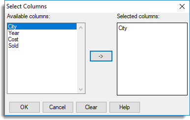
| Select columns for inclusion |
After you click OK this opens a new dialog that lets you select which columns to include in your final spreadsheet.
|
| Sort factor levels | If your data contains factor columns this option will sort the numeric levels (or text labels) into ascending order. |
| Suggest columns to be factors | Genstat will prompt you to convert columns to factors when the column contains x number of repeated values. You can set the number of repeated values in Tools | Spreadsheet Options then click the Conversions tab. Select Suggest converting columns with <=x unique items to factors and set the number as required. |
| Remove empty rows | Remove any rows that contain no data. |
| Remove empty columns | By default, any columns that do not contain data are removed from the Genstat spreadsheet. However, you can keep the empty columns by deselecting this option. |
| Data contains variates & factors only | Any column containing text will be converted to either a variate or factor. If the column contains less than 20% text cells, the column will be made into a variate, otherwise the column will be converted into a factor. |
| Skip first x non-empty rows | The first specified number of rows will be excluded from the spreadsheet. This is useful to exclude any comments that made have been made in the worksheets. Text in these rows can still be used for column names or descriptions – see next option below. |
| Read columns names from file | Controls whether the imported column names are used. Yes if all labels – Read the column names from the row specified in the Column names in row option if all the cells in this row contain labels only or are empty. A default column name will be generated for an empty cell. Yes – Use the cells specified in the Column names in row option . If a cell contains a number, then it will be prefixed with “_” to ensure it is a valid Genstat identifier name. No – Generate default names for the columns, ignoring those in the file. |
| Column names in row | Specifies the row number to use for column names. |
| Column descriptions in row | When selected, the cells in the specified row number will be used for column descriptions. |
| Row numbers (above) are | Controls whether the row numbers are relative to the data range or relate to a whole worksheet. Relative – Row numbers start from the top of the restricted cell range. Absolute – Row numbers start from the top of the worksheet and thus correspond to the absolute row numbering in Excel/Quattro. |
| Text to number | Sometimes numbers are accidentally mistyped as letters. Common mistypings include i, I, l, L for the number 1; o, O for the number 0; a comma for a decimal point, etc. Text to number allows Genstat to convert text labels by substituting numbers for letters or, where this is not possible, the label is converted to a missing value. Strict – Change text strings to numbers only when there are no non-numeric characters in the string. For example, the text ’23’ is converted to 23, the text ‘1a’ contains an alphabetic character so the whole label is converted to a missing value. 1 substitution – Allow a single number to be mistyped and substitute this with the appropriate number. A single lower case ‘o’ or upper case ‘O’ is converted to 0: lower case ‘i’, upper case ‘I’, lower case ‘l’, or upper case ‘L’ is converted to 1. Lower case ‘s’ or upper case ‘S’ is converted to 2. A comma is converted to a decimal point. For example, ‘1o’ contains a single alphabetic character so is converted to 10, ‘1,i’ contains two a comma and an alphabetic characters so is converted to a missing value. Common substitutions – Allows multiple numbers to be mistyped and converts them to the appropriate numbers. For example, ‘LOO’ is converted to 100. Standard – The same as Common substitutions, but any letters at the end of a number are ignored. For example, ’23o’ is converted to 23, ‘i20’ has an alphabetic character at the front so the whole label is converted to a missing value. Lax – Change all text numbers to actual numbers and remove any non-numeric characters. For example, ‘A23X’ is converted to 23. |
| Restricted cell range | Lets you specify a range of cells to import from the worksheet. Type the start and finish cells names separated by a colon, e.g. C1:D96. |
| Add to book | Any open spreadsheets will be displayed in this dropdown list. Select a spreadsheet to insert your data into or leave it at the default setting New Book to create a new workbook. |
| Missing value text | This lets you supply your own text to be inserted into empty cells (the default values are an asterisk * for a variate column or a blank cell for factors and texts). For example, you could use N/A to represent a missing value. |
| Match columns by | Controls how columns are matched between worksheets. Position – matches the worksheet columns by their position i.e. column one in the second worksheet will be appended to column one in the first worksheet, etc. Name – matches and appends worksheet columns that have the same name, regardless of their position. |
| Check for date values | If selected, Genstat checks all text columns to see if they contain data in date format. If any columns appear to contain dates you will be to prompted to convert these to a date format. |
| Set as active sheet |
This sets the new spreadsheet that is created as the active spreadsheet. Setting an active spreadsheet provides a method of avoiding multiple data updates to the server when more than one spreadsheet is open within Genstat. When a spreadsheet is set as the active spreadsheet only data from that spreadsheet is automatically updated to the Genstat server. Another advantage of specifying an active spreadsheet is that the Spread menu options will always be enabled even if your spreadsheet does not have the cursor focus. |
| Ignore case on matching factor labels | If selected, Genstat will match the existing and appended labels even if they use different case e.g. AB and ab will be recognized as the same label. |
VBA to Append Data from multiple Excel Worksheets into a Single Sheet – By Column
Append data from multiple Worksheets into a single sheet By Column using VBA:Project Objective
VBA to Append the data in multiple Worksheets to a newly created Worksheet in the same workbook at the end of the column. The ranges in all worksheets are Append into the ‘Append_Dat’ Worksheet(final Worksheet) one after another in column wise at the end of the column. If data is not available in the Source Worksheet(i.e Input Worksheet) , data will not be updated in the Append_Data(Final) Worksheet. Following is the step by step detailed explanation to automate this process using VBA.
- How we are going to develop this project module(The KEY steps)
- Final VBA Module Code(Macro)
- Function: To Find Last Row
- Function: To Find Last Column
- Instructions to Execute the Procedure
- Download the Project Workbook – Excel Macro File
How we are going to develop this project module(The KEY steps):
To Append all worksheets in the workbook, we have to first create a new worksheet(lets call master sheet) and then loop through each worksheet in the workbook. We have to find the valid data range in each worksheet and Append to the newly created master sheet at the end of the column.
Let me explain the key steps to develop this project. We are going to write a procedure (Append_Data_From_Different_Sheets_Into_Single_Sheet_By_Column) with the below approach.
- Step 1: Declarations: We will declaring required variables and objects which are using in our procedure.
- Step 2: Disable the Screen updating and Events: temporarily to avoid screen flickering and events triggering.
- Step 3: Delete old Master sheet: Before creating new master sheet, we have to check if there is any existing sheet with the same name and delete it.
- Step 4: Adding new worksheet : Lets add new Master sheet(Append_Data Sheet)to paste the data from other sheets
- Step 5: Loop through each sheet: Now,let’s loop through each worksheet (let’s call source sheet) and paste in the master sheet
- Step 5.1: Find Last Available Row: Now we have to find the last available row in the master sheet to paste the data at the end of the column.
- Step 5.2: Find Last used Row and Last used column: Now we have to find the last row and last column of the source sheet
- Step 5.3: Check if there is enough data: The information got from the above step will helps to check if the data is available in the source sheet
- Step 5.4: Copy the data if exist: Now, copy the data from source sheet and Append to the master sheet
- Step 6: Enable the Screen updating and Events: Let’s reset the screen updating and events.
Note: We will be creating two user defined functions which we will be using in the steps 5 to find last row and last columns.
Now, let us see the code for each step:
Step 1: Declaring variables which are using in the entire project.
Dim Sht As Worksheet, DstSht As Worksheet
Dim LstRow As Long, LstCol As Long, DstCol As Long
Dim i As Integer, EnRange As String
Dim SrcRng As Range
Step 2: Disable Screen Updating is used to stop screen flickering and Disable Events is used to avoid interrupted dialog boxes / popups.
With Application
    .ScreenUpdating = False
    .EnableEvents = False
End With
Step 3: Deleting the ‘Append_Data’ Worksheet if it exists in the Workbook. And Display Alerts is used to stop popups while deleting Worksheet.
Application.DisplayAlerts = False
On Error Resume Next
ActiveWorkbook.Sheets("Append_Data").Delete
Application.DisplayAlerts = True
Step 4: Adding a new WorkSheet at the end of the Worksheet. Naming as ‘Append_Data’ . And finally it is assigned it to object (DstSht).
With ActiveWorkbook
    Set DstSht = .Sheets.Add(After:=.Sheets(.Sheets.Count))
    DstSht.Name = "Append_Data"
End With
Step 5: It is looping through each(or all) WorkSheet in the workbook.
And if statement is checking the Input sheet(Input Data) and destination sheet(Append_Data Sheet) is equal or not. If it is equal, then it is going to check next worksheet. If it is not equal to then it copies the input data and Append to Append_Data Worksheet.
For Each Sht In ActiveWorkbook.Worksheets
If Sht.Name <> DstSht.Name Then
End if
Step 5.1: Finding the last column in the ‘Append_Data’ Worksheet using ‘fn_LastColumn ‘ function.
DstCol = fn_LastColumn(DstSht)
Step 5.2: Finding Last used row and Last used column in the Input Worksheet and assigning it to the objects LstRow and LstRow .
Finding Last used cell address in the Worksheet and assigned it to object EnRange . Finally finding Input data range in the Input Worksheet and assigning it to the ‘SrcRng ‘ object.
       LstRow = fn_LastRow(Sht)
       LstCol = fn_LastColumn(Sht)
       EnRange = Sht.Cells(LstRow, LstCol).Address
       Set SrcRng = Sht.Range("A1:" & EnRange)
Step 5.3: Check whether there are enough columns in the ‘Append_Data’ Worksheet. Otherwise it displays message to the user and go to the IfError .
     If DstCol + SrcRng.Columns.Count > DstSht.Columns.Count Then
            MsgBox "There are not enough columns to place the data in the Append_Data worksheet."
            GoTo IfError
        End If
Step 5.4: Copying data from the input Worksheet and appending with destination Worksheet.
SrcRng.Copy Destination:=DstSht.Cells(1, DstCol + 1)
Step 6: Enableing Screen Updating and Events at the end of the project.
With Application
        .ScreenUpdating = True
        .EnableEvents = True
    End With
Final VBA Module Code(Macro):
Please find the following macro to Append data from different Worksheets from the Workbook at the end of the column.
Sub Append_Data_From_Different_Sheets_Into_Single_Sheet_By_Column()
'Procedure to Consolidate all sheets in a workbook

On Error GoTo IfError

'1. Variables declaration
Dim Sht As Worksheet, DstSht As Worksheet
Dim LstRow As Long, LstCol As Long, DstCol As Long
Dim i As Integer, EnRange As String
Dim SrcRng As Range

'2. Disable Screen Updating - stop screen flickering
'   And Disable Events to avoid inturupted dialogs / popups
With Application
    .ScreenUpdating = False
    .EnableEvents = False
End With

'3. Delete the Append_Data WorkSheet if it exists
Application.DisplayAlerts = False
On Error Resume Next
ActiveWorkbook.Sheets("Append_Data").Delete
Application.DisplayAlerts = True

'4. Add a new WorkSheet and name as 'Append_Data'
With ActiveWorkbook
    Set DstSht = .Sheets.Add(After:=.Sheets(.Sheets.Count))
    DstSht.Name = "Append_Data"
End With

'5. Loop through each WorkSheet in the workbook and copy the data to the 'Append_Data' WorkSheet
For Each Sht In ActiveWorkbook.Worksheets
    If Sht.Name <> DstSht.Name Then
       '5.1: Find the last row on the 'Append_Data' sheet
       DstCol = fn_LastColumn(DstSht)

       If DstCol = 1 Then DstCol = 0

       '5.2: Find Input data range
       LstRow = fn_LastRow(Sht)
       LstCol = fn_LastColumn(Sht)
       EnRange = Sht.Cells(LstRow, LstCol).Address
       Set SrcRng = Sht.Range("A1:" & EnRange)

       '5.3: Check whether there are enough columns in the 'Append_Data' Worksheet
        If DstCol + SrcRng.Columns.Count > DstSht.Columns.Count Then
            MsgBox "There are not enough columns to place the data in the Append_Data worksheet."
            GoTo IfError
        End If

      '5.4: Copy data to the 'Append_Data' WorkSheet
        SrcRng.Copy Destination:=DstSht.Cells(2, DstCol + 1)
    End If
Next
DstSht.Range("A1") = "You can place the heading in the first column"

IfError:
'6. Enable Screen Updating and Events
    With Application
        .ScreenUpdating = True
        .EnableEvents = True
    End With

End Sub
Below are the two user defined functions which we have created to find the last row and last column of the given worksheet. We have called these functions in the above procedure at step 5.1 and 5.2.
Function to Find Last Row:
The following function will find the last row of the given worksheet. ‘fn_LastRow’ will accept a worksheet(Sht) as input and give the last row as output.
'In this example we are finding the last Row of specified Sheet
'In this example we are finding the last Row of specified Sheet
Function fn_LastRow(ByVal Sht As Worksheet)

    Dim lastRow As Long
    lastRow = Sht.Cells.SpecialCells(xlLastCell).Row
    lRow = Sht.Cells.SpecialCells(xlLastCell).Row
    Do While Application.CountA(Sht.Rows(lRow)) = 0 And lRow <> 1
        lRow = lRow - 1
    Loop
    fn_LastRow = lRow

End Function
Function to Find Last Column:
The following function will find the last column of the given worksheet. ‘fn_LastColumn’ will accept a worksheet(Sht) as input and give the last column as output.
'In this example we are finding the last column of specified Sheet
Function fn_LastColumn(ByVal Sht As Worksheet)

    Dim lastCol As Long
    lastCol = Sht.Cells.SpecialCells(xlLastCell).Column
    lCol = Sht.Cells.SpecialCells(xlLastCell).Column
    Do While Application.CountA(Sht.Columns(lCol)) = 0 And lCol <> 1
        lCol = lCol - 1
    Loop
    fn_LastColumn = lCol

End Function
Instructions to Execute the Procedure:
You can download the below file and see the code and execute it. Or else, you create new workbook and use the above code and test it. Here are the instructions to use above code.
- Open VBA Editor window or Press Alt+F11.
- Insert a new module from the Insert menu.
- Copy the above procedure and functions and paste it in the newly created module.
- You can enter some sample data in multiple sheets. and run the procedure.
Download the Project Workbook – Excel Macro File<:
Here is the example Excel macro Workbook to explore yourself.
Consolidate data from different sheets By Column
A Powerful & Multi-purpose Templates for project management. Now seamlessly manage your projects, tasks, meetings, presentations, teams, customers, stakeholders and time. This page describes all the amazing new features and options that come with our premium templates.
Save Up to 85% LIMITED TIME OFFER

All-in-One Pack
120+ Project Management Templates
Essential Pack
50+ Project Management Templates
Excel Pack
50+ Excel PM Templates
PowerPoint Pack
50+ Excel PM Templates
MS Word Pack
25+ Word PM Templates
Ultimate Project Management Template
Ultimate Resource Management Template
Project Portfolio Management Templates
VBA Reference
Effortlessly
Manage Your Projects
120+ Project Management Templates
Seamlessly manage your projects with our powerful & multi-purpose templates for project management.
120+ PM Templates Includes:
2 Comments
-
sunil
September 18, 2016 at 10:17 PM — Replygiven procedure moves all the contents of the worksheets. I want to move only referenced cell content to get a report. How can this be achieved. say for example range c4:c9, F9:G9, B13:f45.
-
Jyoti
April 30, 2019 at 5:08 PM — ReplyVery useful stuff, Thanks very much for sharing
Effectively Manage Your
Projects and Resources
ANALYSISTABS.COM provides free and premium project management tools, templates and dashboards for effectively managing the projects and analyzing the data.
We’re a crew of professionals expertise in Excel VBA, Business Analysis, Project Management. We’re Sharing our map to Project success with innovative tools, templates, tutorials and tips.
Project Management
Excel VBA
Download Free Excel 2007, 2010, 2013 Add-in for Creating Innovative Dashboards, Tools for Data Mining, Analysis, Visualization. Learn VBA for MS Excel, Word, PowerPoint, Access, Outlook to develop applications for retail, insurance, banking, finance, telecom, healthcare domains.
Page load link
Go to Top

Working with Tables is great. I mean, did you even see where you’re at? Our name says it all. But sometimes they just don’t work quite like you would think. As in life, we work with what we have. A lot of people work with Tables and just want them to work how they would imagine. You know, intuitively. We do too.
Today we’re focusing on a topic which has had people scratching their head for several years—in fact, since Tables were reinvented in 2007! Adding data below a Table, specifically with the Totals Row showing. You might be asking yourself, “doesn’t Excel already do this?” Well, kind-of-sort-of-but-not-really. As you can see in the below image, with no Total Row, data which is entered directly below a Table will get consumed into that Table no problem. This works as a person would expect, or at least how we would expect.
Appending new rows with no Total Row

Now if you want to use a Total Row, because, well, why not, then it’s not so straight forward, but you can still do it. In the image below you can see where you need to grab the lower-right Table indicator and drag it down to consume those new rows. The new rows will be consumed into the Table and the Total Row will appear in the proper place, switching with those newly consumed rows.
Appending new rows with Total Row

While the first image above will work automatically as you type, the second image above will not and requires an extra click-and-drag to make it happen. We’re lazy. If things should happen automatically and they don’t, in fact requiring more work from us, then we generally whip out the code and make our lives easier by coding it ourselves. This is what we’ve done here. The code below will automatically add rows of data once entered below your Table when the Total Row is showing.
Note: If your Total Row is not showing, the behavior will be that of native Excel, and rows will be consumed into your Table until it cannot figure out if you want the rows consumed into the Table or not.
Appending new rows with fancy-dancy code

This code belongs in the Worksheet module of the desired sheet to add this functionality to. If you need to know how to add this code, check out our cool Canadian over at Contextures for assistance.
There are two constants declared at the top of this code.
- SingleRowOnly. This specifies whether multiple rows should be included in appending into the Table, or if only a single row should be.
- MaxRowCount. As to not go crazy with appending rows to a Table automatically, this is the maximum number of rows to include at any one time. If SingleRowOnly is set to True, this constant is moot.
|
1 2 3 4 5 6 7 8 9 10 11 12 13 14 15 16 17 18 19 20 21 22 23 24 25 26 27 28 29 30 31 32 33 34 35 36 37 38 39 40 41 42 43 44 45 46 47 48 49 50 51 52 53 54 55 56 57 58 59 60 61 62 63 64 65 66 67 68 69 70 71 72 73 74 75 76 |
Option Explicit Private Const SingleRowOnly As Boolean = False Private Const MaxRowCount As Long = 100 Private Sub Worksheet_Change(ByVal Target As Range) Dim ResizeRange As Range Dim Table As ListObject Dim TotalsShowing As Boolean Dim ExpandTables As Boolean Dim RowIndex As Long Dim RowCount As Long ‘ Make sure sheet isn’t protected If Me.ProtectContents Then Exit Sub ‘ If already in a table, then exit If Not Target.ListObject Is Nothing Then Exit Sub ‘ Make sure only one row is being changed If Target.Rows.Count > 1 Then Exit Sub ‘ Make sure we’re not in row 1 If Target.Row = 1 Then Exit Sub ‘ Make sure we’re in the row right under the Totals row If Target.Offset(—1, 0).ListObject Is Nothing Then Exit Sub ‘ Set table Set Table = Target.Offset(—1, 0).ListObject TotalsShowing = Table.ShowTotals ExpandTables = Application.AutoCorrect.AutoExpandListRange ‘ If Totals not showing, exit If Not TotalsShowing Then Exit Sub ‘ Make sure the selection is a contiguous range If Target.Areas.Count > 1 Then Exit Sub ‘ Make sure Target range is within the table columns If Target(1, 1).Column < Table.ListColumns(1).Range.Column Then Exit Sub If Target(1, Target.Columns.Count).Column > Table.ListColumns(Table.ListColumns.Count).Range.Column Then Exit Sub ‘ Prepare to adjust table Application.EnableEvents = False Table.ShowTotals = False Application.AutoCorrect.AutoExpandListRange = True ‘ Set the resize range If WorksheetFunction.CountA(Table.Range(1, 1).Offset(Table.Range.Rows.Count + 1).Resize(1, Table.Range.Columns.Count)) > 0 Then If Not SingleRowOnly Then RowIndex = Target.Row RowCount = RowIndex Do Until WorksheetFunction.CountA(Me.Range(Me.Cells(RowCount, Table.Range(1, 1).Column), Me.Cells(RowCount, Table.Range(1, Table.ListColumns.Count).Column))) = 0 Or RowCount — RowIndex > MaxRowCount RowCount = RowCount + 1 Loop Set ResizeRange = Table.Range.Resize(Table.Range.Rows.Count + RowCount — RowIndex, Table.Range.Columns.Count) Else Set ResizeRange = Table.Range.Resize(Table.Range.Rows.Count + 1, Table.Range.Columns.Count) End If Else Set ResizeRange = Table.Range.Resize(Table.Range.Rows.Count + 1, Table.Range.Columns.Count) End If ‘ Make table adjustment Table.Resize ResizeRange ‘ Put things back the way we found them Application.AutoCorrect.AutoExpandListRange = ExpandTables Table.ShowTotals = TotalsShowing Application.EnableEvents = True End Sub |
In the above code we’ve done what we think is good housekeeping. We’ve taken inventory of the Table settings at the start, then set them back when we’re done.
Another solution to this would be to Unlist the Table, then re-create it. We don’t recommend this because if you have calculated columns or dependent references pointing to structured references of the Table, they will get forced to standard cell referencing (absolute) and will not go back to structured referencing automatically. Because of this is why we work within the confines of keeping it a Table.
TL;DR
Copy code above to worksheet module. Enjoy automatically having rows be appended to Table with your Total Row showing.