
When you’re looking up text or values you’ll often want to use wildcards in your searches.
The wildcards are:
- * (Asterisk)
- ? (Question Mark)
- <> (Less Than, Greater Than)
- (blank)
Wildcards work with all of the following functions:
- SUMIF, SUMIFS
- COUNTIF, COUNTIFS
- AVERAGEIF, AVERAGEIFS
- VLOOKUP, HLOOKUP (‘<>’ will not work with these)
- MATCH (‘<>’ will not work with this)
Lets look at the wildcard combinations using the SUMIF function. The arguments for SUMIF are: RANGE, CRITERIA and SUM_RANGE. RANGE is where we’re going to look for our criteria. CRITERIA is what we’re looking for (this will include our wildcards). SUM_RANGE is the range of data to sum when the criteria is matched in the range.
Below we look at these examples: “” , “*” , “<>*” , “*A*” , “<>*A*” , “???” , “A?” , “*300*” , “<>B” , “<>A?” , “<>” , “<>???”
To start, check Fig(a1) for the table we’ll use when analyzing the wildcard results. This table shows also shows the results for SUMIF with 300 as the criteria.

Fig(a1)
It is worth noting that the result includes cell B22 even though this is formatted as text. This might be surprising so it is worth being aware of. Other than that, as expected this sums all cells in the range that equal 300. It doesn’t matter if cell B26 is formatted as text or a number, the result of the SUMIF is unaffected.
Now lets look at the wildcard examples.
1. SUMIF Blank [criteria “” = BLANK cells]
If we use a blank criteria the SUMIF will sum all the blanks (cell B9 in this case).
COUNTIF works in the same way with BLANK criteria. This may be useful to identify any blank cells in a list. You may want to consider this as a validation check in your spreadsheets. Either to check users have entered all relevant cells. Or to check that data you’ve imported to Excel is complete.
Note: these BLANK cells could include formulas that are returning blank text. Such as =IF($A$1 = 1, 1, “”)

Fig(a2)
2. Excel Wildcard Asterisk “*” [criteria “*” = TEXT cells]
The asterisk is a wildcard for any text in the search for matching cells. When used on its own as in this case it returns any cell with text.
On its own it therefore excludes all blank cells (as well as excluding any numeric cells). Again this can be a useful validation. While the example above was checking for blank cells, this time we’re also excluding numeric values from the result.
The rows summed are shown in yellow.

Fig(a3)
3. Wildcard Asterisk Preceded By “<>*” [criteria“<>*” = NON-TEXT cells]
Now if we add ‘<>’ to the asterisk wildcard we can get the opposite result. So ‘<>*’ will return a sum of all the numeric cells (including any blanks in the range).

Fig(a4)
If you want a count of numeric values only in range $B$7:$B$22 then you can use this wildcard example then deduct the blank count: “=COUNTIF($B$7:$B$22,”<>*”) – COUNTIF($B$7:$B$22,””)”
4. Combining Asterisk Wildcard With Text [criteria“*A*” = text with ‘A’ somewhere in string]
Lets check our list for ‘*A*’. This is one of the most common uses of wildcards in Excel, particularly with VLOOKUP or SUMIF. You can see below that anything with ‘A’ is found and the range in column C is summed. This is not case sensitive.

Fig(a5)
5. Wildcard to Exclude Anything With ‘A’ in Cell [criteria“<>*A*” = cells with no ‘A’]
Reversing the wildcard in 4. above. We just add ‘<>’ to the previous string. So ‘<>*A*’ is going to result in a sum of all cells that don’t have ‘A’ in their value. This sum includes the blank cell B9 as this also fulfills the criteria of not containing ‘A’ in its value.

Fig(a6)
6. The Question Mark Wildcard [criteria“???” = text with exactly 3 characters length]
Again this is commonly used. While the asterisk ‘*’ represented any number of characters, the question mark ‘?’ is just going to represent a single character. In the example below we’ll use ‘???’. As it only counts text, the 3 digit numbers are not included in the result. That being the case, only cell B13 meets this criteria.

Fig(a7)
7. Another Question Mark Wildcard Example [criteria“A?” = text which starts with ‘A’ followed by exactly one character]
In this example we’ve joined the question mark ‘?’ wildcard with text ‘A?’. As it counts as just one character the SUMIF includes only two character values that start with ‘A’. The only cell in our range that meets this criteria is cell B12.

Fig(8)
8. Combining Asterisk ‘*’ Wildcard with A Number [criteria“*300*” = text with ‘300’ in string]
If you’ve been following along so far it may not be surprising that ‘*300*’ is just going to pick up text with ‘300’ in the string. Any numbers with 300 are going to be excluded from the result.

Fig(a9)
9. Excluding Strings [criteria“<>B” = text which aren’t “B”]
Lets try excluding all cells in the range that equal ‘B’. Following our logic this is simply ‘<>B’.

Fig(a10)
10. Exclude All Cells With ‘A’ Followed by One Character [criteria“<>A?” = any cell that isn’t ‘A’ followed by one character]
Again we just need to take our string to identify ‘A’ followed by one character and precede it with ‘<>’.

Fig(a11)
11. All Non-Blank Cells [criteria“<>” = NON-BLANKS]
We can find all non-blank cells by using the exclude ‘<>’ wildcard on its own.

Fig(a12)
12. Exclude All 3 Character Text Strings [criteria“<>???” = cells that aren’t 3 character text]
We’re going to use ‘<>???’ in our last example. The exclusion picks up the text strings that are 3 characters long. However, numeric numbers are ignored so they are not excluded from the answer.

Fig(a13)
Work smarter in Excel with our productivity tools.
Conclusion
Hopefully these examples are enough to see the options. It is important to consider what is being excluded or included. Particularly with regard to numeric cells and blanks. As well as being powerful SUMIF criteria, these can become an excellent validation check in your spreadsheets by using COUNTIF and COUNTIFS functions.
Just to recap these examples:
- “” (or blank) will match blank cells
- “*” will match any cell with text (blank cells are not matched)
- “<>*” this is the opposite of 2. above so all numeric and blank cells meet the criteria
- “*A*” will match any cell with ‘A’ in its value (this is not case sensitive)
- “<>*A*” is the opposite of 4. above so you can easily exclude text from the match
- “???” as the question mark represents a single character you can match all cell values that are 3 characters long (provided they are text)
- “A?” will provide all provide matches of any cell that begins with ‘A’ and is 2 characters long
- “*300*” similar to 4. above this will match any cell formatted as text that has ‘300’ somewhere in its string.
- “<>B” to match all cells except those that are “B”
- “<>A?” to match all cells except those that begin “A” and are two characters long
- “<>” all cells that are no blank
- “<>???” all cells that are not text and 3 characters long
Learn more about use of wildcards with this example: Lookup Part of Text in a Cell
Subscribe for exclusive tips
Can you use wildcards in Excel formulas?
Yes. Wildcards work with these functions: SUMIF, SUMIFS, COUNTIF, COUNTIFS, AVERAGEIF, AVERAGEIFS, VLOOKUP, HLOOKUP, MATCH
What is the symbol for ‘any’ (NOT BLANK) value in Excel?
Use the asterisk (*) to represent ‘any’ value.
How do you use wildcards?
In an appropriate Excel function, use a wildcard to represent other characters. E.g. to count cells that start with «B» in cells A1 to A20: ‘=COUNTIF($A$1:$A$20,»B*»)’
How do you do a wildcard search in Excel?
From the ‘HOME’ menu select ‘Find & Select’ then ‘Find…’. Now type your search term using * to replace any number of characters or ? to replace single characters
What is the symbol for ANY NUMBER in Excel?
Use the less than, greater than and asterisk together (<>*) to represent ‘any’ numbers (includes blanks).
In this tutorial, you will be provided with detailed guidance to:
- Understanding the Number Format Code
- Create Custom Symbols in Excel
Watch it on YouTube and give it a thumbs-up!

Excel has several in-built features to create custom formatting to your numbers. But if none of them meets your requirement, you will have to create your own.
The key benefit of adding custom formatting is that it only controls how the number is displayed without changing the underlying value of that number.
A cool feature within Excel is the ability to format a cell’s value by pressing CTRL + 1 on any cell. This brings up the Format Cells dialogue box and under the Custom category, you can customize the Type to whatever you like.
You can even create custom symbols in Excel using this feature!
But before you understand how to add a symbol to a number in Excel, you need to first know how to write a number format code.
Understanding the Number Format Code
You can change the format of a cell’s value by either using various formats available in Excel or creating a custom format using number format code.
Number format code is created using symbols that tells Excel how you want to display the cell’s value. When adding a custom format in Excel, there are four formatting sections that you have to follow:
Positive format; Negative format; Zero format; Text format.
Each of these sections is separated by a semicolon(;) and only the first section is required to create a custom format.
You can view the Custom Number Formats blog post that explains this in more detail here
Create Custom Symbols in Excel
Now that you have understood the structure of how to use number format code, let’s use that knowledge and learn how to insert symbol in excel formula based on the cell’s value.
Working with an example will make this concept more clear. So, let’s get started.
Follow the step-by-step tutorial below to know how to add a symbol in excel formula and make sure to download the exercise workbook to follow along:
DOWNLOAD EXCEL WORKBOOK
Example #1:
In the table below, you have daily temperature recorded and you want to add symbol °C to it.

You want to add “°C” symbol to the temperature column and the edited table like this:

The following steps should be incorporated to create custom symbols in Excel:
STEP 1: Select the “Temperature” column

STEP 2: Go to Home > Under Format Dropdown, Select More Number Formats

STEP 3: In the Format Cell dialog box, select Custom

STEP 4: In the type section, type 0.00 °C and Click OK

This is how the edited table will look like.
Example #2:
In Example #1, you have learned how to add symbols in Excel irrespective of the cell’s value. Now let’s move forward and understand how to add symbols based on the number stored in the cell.
So, the symbols added would be based on the value stored in the cell.
In the table below, you have the status for different projects listed below with “0″ indicating Completed and “-1” indicating Pending.

Now you want to create custom symbols in Excel i.e. you want to add custom symbol :
- ✓ Completed; when status is 0
- ✕ Pending; when status is -1
The table with custom symbols should look like this:

STEP 1: Select the Status Column

STEP 2: Press Ctrl +1 to open the Format Cells dialog box

STEP 3: Select the Custom category and select a number format type – ✓” Completed”;✕” Pending”. This will change the format to ✓ Completed when cell value is 0 and ✕ Pending when cell value is -1.
You can also add color to make the formatting more distinct. Use the format type – ✓” Completed”[Green];[Red]✕” Pending” to add green color to the completed project and red to pending projects.

This is how the table will look like this.

Example #3:
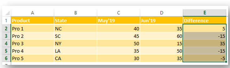
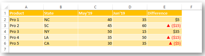
Here, you have monthly sales, estimates benchmark sales and variance calculated.

You want the % Variance column in our data to have symbols ▲▼ to show a negative and positive variance. So, you have the % variance value customized as below:
- Green in color with ▲ symbol; when variance % is positive
- Red in color with ▼ symbol; when variance % is negative
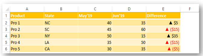
The table should look something like this:

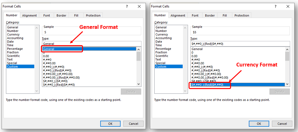
STEP 1: Enter a Variance calculation in a column, select the column’s variance numbers and press CTRL + 1 to bring up the Format Cells dialogue box

STEP 2: Select the Custom category and select a number format type – “#,##0;[Red]-#,##0

The first section of this code #,##0 is for a positive number, and second code [Red]-#,##0 is for a negative number.
To show the positive number in green color and add a % sign, follow Step 3.
STEP 3: Under the Type: area you will need to enter the text [green] at the start of the positive value string and enter the % sign at the end of the positive and negative value strings
![]()
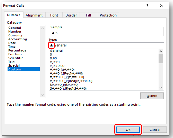
STEP 4: Now select a blank cell and go to Insert > Symbol > Font: Arial > Subset: Geometric Shapes and then Insert the Up-Pointing Triangle and Insert the Down-Pointing Triangle and press Cancel

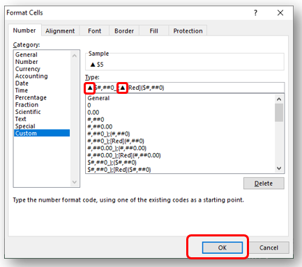
STEP 5: You will need to copy the triangles, select the variance numbers, press CTRL + 1 and paste the triangles before each positive and negative value string, then press OK

You now have your custom number formats with an upwards triangle for any positive %s and a downwards triangle for any negative %s


Make sure to download our FREE PDF on the 333 Excel keyboard Shortcuts here:

You can learn more about how to use Excel by viewing our FREE Excel webinar training on Formulas, Pivot Tables, and Macros & VBA!
You can follow our YouTube channel to learn more about How To Use Excel efficiently!
How to Insert Symbol in Excel?

Have you ever faced the challenge of using special character symbols in number formatting or customized number formatting?
It is easy to insert any symbol in numbers i.e Delta Symbol or Special Character Symbols in Excel Number Formatting.
You may easily do this by below steps:
Inserting Symbols in Numbers
-
Select the Cells or Column where you want numbers to be shown with Delta (▲) symbol
-
Right Click on the selected Cells and click on “Format Cells”
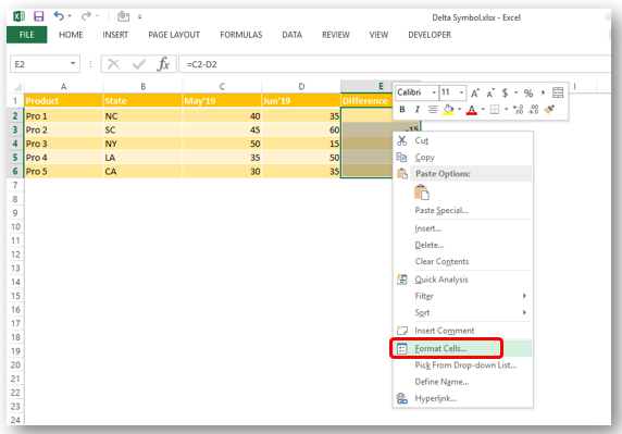
-
Select Custom format under Number Menu as shown below:
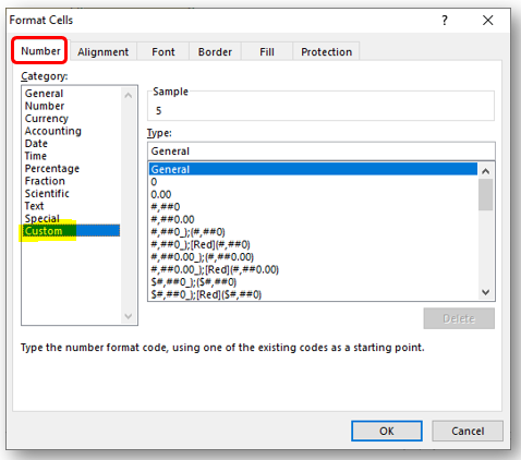
-
So here you will see the number format of your data. I have shown two samples here with different number format:
To Insert Symbol In Excel: 2 types of Formatting
-
You will mostly find two types of formatting under «Custom Format» as shown in above image eitheri) General Formatting
ii) Currency FormattingThough there are many other formatting available as per your data however you may insert symbols using this method easily. So lets continue 🙂
i) General Number Formatting in Excel
So Click at the beginning of “General” as shown below and insert “Delta Symbol” either:
-
You may copy the below Delta (▲) sign and paste it at the beginning and press Space Key after Delta Sign (▲), if you want to see gap between the sign and number. You may copy any of the symbol as below and use same method:
-
Or you can enter it by Holding ALT Key and press 3 & 0 in sequential manner. Do you want to know more shortcuts for inserting Special Characters Symbols ? Click at below link:
ii) Custom Currency Number Formatting in Excel
In Currency Number Formatting or Accounting Number Formatting, there are two parts of format i) for Positive Number ii) Negative Number. So you need to insert it twice if you want to show Special Symbols for both formats else only at the beginning of Negative Or Positive Format. Lets go through below:
-
You may copy the below Delta (▲) sign and paste it at the beginning and press Space Key after Delta Sign (▲), if you want to see gap between the sign and number. You may copy any of the symbol as below and use same method:
-
Or you can enter it by Holding ALT Key and press 3 & 0 in sequential manner. Do you want to know more shortcuts for inserting Special Characters Symbols ? Click at below link:
-
Now if you see at below image, you will observe that I inserted the Delta (▲) symbol twice because here currency format contains two format:i) One is for Positive (+) “$#,##0_)”
ii) and one is for Negative (-) “[Red]($#,##0)”. Red is a color of the number when shows Negative (-)Both the formats are separated by “;” in this below format

-
So we need to add the Delta sign as described at the beginning on both the Formats and it should look like as below:▲ $#,##0_);▲ [Red]($#,##0)
If you want to see Delta (▲) sign only for Negative numbers. So you should add the symbol only on Negative Format and it should be as below:
▲ $#,##0_);▲ [Red]($#,##0)
-
You will see your numbers will be changed and contain Delta Sign similar below:
Negative numbers with Delta Sign in Excel
Other Special Charcters Symbol
You may insert any special character symbols using this method in Number formatting
Did this article solve your query? Please comment at below box, if you find any challenge.
Have a great day ahead 🙂
Recommended Articles
- How does Histogram work in Excel? (Definitive Guide)
- Create Pareto Chart in Excel
- Find Duplicates in Excel
- Few Simple Excel Tips-Excel Learners should know
- Impress Your Clients by Hiding these Simple Features
Excel VBA Course : Beginners to Advanced
We are currently offering our Excel VBA Course at discounted prices. This courses includes On Demand Videos, Practice Assignments, Q&A Support from our Experts. Also after successfully completion of the certification, will share the success with Certificate of Completion
This course is going to help you to excel your skills in Excel VBA with our real time case studies.
Lets get connected and start learning now. Click here to Enroll.
Secrets of Excel Data Visualization: Beginners to Advanced Course
Here is another best rated Excel Charts and Graph Course from excelsirji. This courses also includes On Demand Videos, Practice Assignments, Q&A Support from our Experts.
This Course will enable you to become Excel Data Visualization Expert as it consists many charts preparation method which you will not find over the internet.
So Enroll now to become expert in Excel Data Visualization. Click here to Enroll.
![]()
List of Symbols in Excel and Usage

Here are the list of symbols used in Excel. Symbols in Excel are very useful to represent the important information using signs in Excel. It helps the users to enhance the representation of the information for easy understanding of the data. We can provide more meaning to the data using verity of symbols. signs, characters and alt codes provided in Excel.
- List of Symbols Available in Excel
- Symbol Dialog Box
- Usage of Symbols in Excel
- Inserting Symbols in a Cell
- Adding to a Number
- Adding in a Chart
- Shortcut to Excel Symbols
- Alt Codes
- Symbols and Functions
- Symbols Cheat Sheet
- Symbols in PDF
- Symbols in Excel Workbook
List of Symbols Available in Excel
Symbol Dialog Box
Usage of Symbols in Excel
Inserting Symbols in a Cell
Adding to a Number
Shortcut to Excel Symbols
Alt Codes
Excel Symbols and Functions
Excel Symbols Cheat Sheet
Excel Symbols pdf
List of Symbols in Excel
Here is the list of useful symbols in Excel. You can quickly have a look and use the required symbol which suites your data. It is very important to note that you know the meaning of the symbol before inserting the symbol in Excel. There are verity of the symbols available in Excel, standard built-in symbols, Special Characters and Custom Fonts. You can browse all the available symbols including Webdings and Wingdings Fonts in the Excel using Symbol Dialog Box.
Excel Symbols Cheat Sheet
Click to View the Full Size Image.
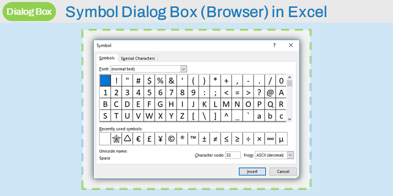
Symbol Dialog Box
Excel is provided with an easy to use Dialog box to browse all the list of symbols available. We can open the Symbol Dialog Box to view, browse and insert the symbols in Excel.
Where is Symbol Command in Excel Ribbon
Symbol Command is available in Insert Ribbon Menu in The Excel. You can see the two commands in Symbols Ribbon Group, they are Equation and Symbol commands.
How to Open Symbol Dialog Box
Follow the below steps to Open Symbol Dialog Box in Excel. You open using Ribbon Command or using Excel Shortcut Keys.
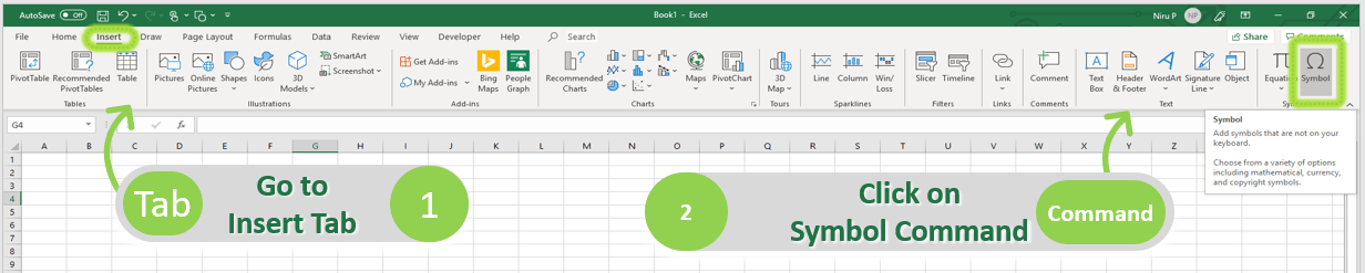
Ribbon Command to Open Symbol Dialog Box:
- Go to Insert Tab in the Excel Ribbon Menu
- Click on the Symbol Command Control button in the Symbols group
- This will Launch the Symbol Dialog Box
Shortcut Key to Open Symbol Dialog Box:
You can press shortcut keys Alt+N+U to open the Symbol Dialog Box.
- Press the ALT Key and Letter N Key
- Then Press the Letter U Key to Open the Dialog Box
Using Symbols with Formulas
We use Excel Formulas in Excel Cell to produce new data based on other Cells in Excel. For example, we can calculate total sales based on Quantity and Price of a product. And we can show the result with a currency symbol. We can use CHAR function and concatenate to any expression of Excel Formula as show below.
Let us say, we have Quantity 25 in Cell A1 and Unit Price $45.80 in Cell B1. The following formula produces the total value in Cell C1.
C1=CHAR (36) &”(USD)” &A1*B1
This will display “$(USD) 1145” in Cell C1.
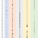
Function to Create List of Symbols in Excel
We can use CHAR function to create a list of function in Excel. We can pass an ASCII code as input parameter to the function. It will return the respective Symbol for the given code. We can pass any value from 0 to 255 in Excel Char Function to return the Special Character Symbols.
Share This Story, Choose Your Platform!
© Copyright 2012 – 2020 | Excelx.com | All Rights Reserved
Page load link
HTTA is reader supported. When you buy through links on our site, we may earn an affiliate commission at no extra cost to you. Learn more.
In today’s article, you’ll learn how to use some keyboard shortcuts to type the Numero Sign or Number Symbol [№] (text) in Word/Excel using the Windows PC.
Just before we begin, I’ll like to tell you that you can also use the button below to copy and paste the Numero sign into your work for free.
However, if you just want to type this symbol on Word with your keyboard, the actionable steps below will show you everything you need to know.
Related Post: How to type Hash (#) or Number sign on Keyboard
Number Symbol [№] Quick Guide
To type the Number Symbol [№] in Microsoft Word, open your MS Word document, press down the Alt key, and type 8470 using the numeric keypad, then release the Alt key.
Below table contains all the information you need to type this Symbol in Word using the keyboard.
| Symbol Name | Numero Sign |
| Symbol Text | № |
| Alt Code | 8470 |
| Shortcut | Alt+8470 |

The quick guide above provides some useful shortcuts and alt codes on how to type the Number Symbol [№] in Word.
For more details, below are some other methods you can also use to insert this symbol into your work such as Microsoft Word or Excel document.
How to type Number Symbol [№] [text] in Word/Excel
Microsoft Office provides several methods for typing Number Symbol [№] or inserting symbols that do not have dedicated keys on the keyboard.
In this section, I will make available for you several different methods you can use to type or insert this and any other symbol on your PC, like in MS Office (ie. Word, Excel, or PowerPoint) for Windows users.
Without any further ado, let’s get started.
Using the Number Symbol [№] Alt Code
The Number Symbol [№] alt code is 8470.
Even though this Symbol has no dedicated key on the keyboard, you can still type it on the keyboard with the Alt code method.
To do this in Word, press and hold the Alt key whilst pressing the Numero Alt code (i.e. 8470) using the numeric keypad.

This method works on Windows only. And your keyboard must also have a numeric keypad.
Below is a break-down of the steps you can take to type the Numero Sign on your Windows PC:
- Place your insertion pointer where you need the Number Symbol [№] text.
- Press and hold one of the Alt keys on your keyboard.
- Whilst holding on to the Alt key, press the Number Symbol [№]’s alt code (8470). You must use the numeric keypad to type the alt code. If you are using a laptop without a numeric keypad, this method may not work for you. On some laptops, there’s a hidden numeric keypad which you can enable by pressing Fn+NmLk on the keyboard.
- Release the Alt key after typing the Alt code to insert the Symbol into your document.
This is how you may type this symbol in Word using the Alt Code method.
Using the Number Symbol [№] Shortcut in Word
The Number Symbol [№] shortcut in MS Word is 2116, Alt+X.
Obey the following instructions to use this shortcut:
- First Launch your MS Word.
- Place the insertion pointer where you need the symbol.
- Type 2116 on your keyboard, then press Alt + X.
This will convert the code (2116) into the Number Symbol [№] at where you place the insertion pointer.
This is how you may insert this symbol using this shortcut.
Copy and Paste Numero Sign – [№] (text)
Another easy way to get the Number Symbol [№] on any PC is to use my favorite method: copy and paste.
All you have to do is to copy the symbol from somewhere like a web page, or the character map for windows users, and head over to where you need the symbol (say in Word or Excel), then hit Ctrl+V to paste.
Below is the symbol for you to copy and paste into your Word document. Just select it and press Ctrl+C to copy, switch over to Microsoft Word, place your insertion pointer at the desired location, and press Ctrl+V to paste.
№
Alternatively, just use the copy button at the beginning of this post.
Using insert Symbol dialog box (Word, Excel, PowerPoint)
The insert symbol dialog box is a library of symbols from where you can insert any symbol into your Word document with just a couple of mouse clicks.
Obey the following steps to insert this symbol ([№]) in Word or Excel using the insert symbol dialog box.
- Open your Word document.
- Click to place the insertion pointer where you wish to insert the symbol.
- Go to the Insert tab.

- In the Symbols category, click on the Symbol drop-down and select the More Symbols button.

The Symbol dialog box will appear.
- To easily locate the Number Symbol [№], go to the font drop-down and select Segoe UI Symbol from the list, then type 2116 in the character code field at the bottom area of the window. After typing this character code, the Number Symbol [№] will appear selected.
- Now click on the Insert button to insert the symbol into your document.

- Close the dialog.
The symbol will then be inserted exactly where you placed the insertion pointer.
These are the steps you may use to insert this Symbol in Word.
Conclusion
As you can see, there are several different methods you can use to type the Numero Sign in Microsoft Word.
Using the shortcut makes the fastest option for this task. Shortcuts are always fast.
Thank you very much for reading this blog.
If you have anything thing to say or questions to ask concerning this guide, please drop it in the comments section below this article.