
Содержание
- Using IF with AND, OR and NOT functions
- Examples
- Using AND, OR and NOT with Conditional Formatting
- Need more help?
- See also
- Использование ЕСЛИ с функциями И, ИЛИ и НЕ
- Примеры
- Использование операторов И, ИЛИ и НЕ с условным форматированием
- Дополнительные сведения
- См. также
- AND function
- Example
- Examples
- Need more help?
- How to use Conditional Formatting
- What is Conditional Formatting
- Fundamentals of Conditional Formatting
- Highlight Cells using rules (if the quantity is greater than 200)
- Highlight cells that contain text
- Editing a conditional formatting rule
- Delete a conditional formatting rule
- Conditional Formatting and Formulas
- How do I highlight the lowest 3 values in Excel?
- How to conditional format if the cell is blank?
- How to use Conditional Formatting to highlight past due dates in Excel
- How to highlight overlapping dates in Excel
- Final thought
- Ultimate Dashboard Tools
Using IF with AND, OR and NOT functions
The IF function allows you to make a logical comparison between a value and what you expect by testing for a condition and returning a result if that condition is True or False.
=IF(Something is True, then do something, otherwise do something else)
But what if you need to test multiple conditions, where let’s say all conditions need to be True or False ( AND), or only one condition needs to be True or False ( OR), or if you want to check if a condition does NOT meet your criteria? All 3 functions can be used on their own, but it’s much more common to see them paired with IF functions.
Use the IF function along with AND, OR and NOT to perform multiple evaluations if conditions are True or False.
IF(AND()) — IF(AND(logical1, [logical2], . ), value_if_true, [value_if_false]))
IF(OR()) — IF(OR(logical1, [logical2], . ), value_if_true, [value_if_false]))
IF(NOT()) — IF(NOT(logical1), value_if_true, [value_if_false]))
The condition you want to test.
The value that you want returned if the result of logical_test is TRUE.
The value that you want returned if the result of logical_test is FALSE.
Here are overviews of how to structure AND, OR and NOT functions individually. When you combine each one of them with an IF statement, they read like this:
AND – =IF(AND(Something is True, Something else is True), Value if True, Value if False)
OR – =IF(OR(Something is True, Something else is True), Value if True, Value if False)
NOT – =IF(NOT(Something is True), Value if True, Value if False)
Examples
Following are examples of some common nested IF(AND()), IF(OR()) and IF(NOT()) statements. The AND and OR functions can support up to 255 individual conditions, but it’s not good practice to use more than a few because complex, nested formulas can get very difficult to build, test and maintain. The NOT function only takes one condition.

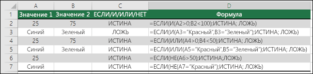
Here are the formulas spelled out according to their logic:
=IF(AND(A2>0,B2 0,B4 50),TRUE,FALSE)
IF A6 (25) is NOT greater than 50, then return TRUE, otherwise return FALSE. In this case 25 is not greater than 50, so the formula returns TRUE.
IF A7 (“Blue”) is NOT equal to “Red”, then return TRUE, otherwise return FALSE.
Note that all of the examples have a closing parenthesis after their respective conditions are entered. The remaining True/False arguments are then left as part of the outer IF statement. You can also substitute Text or Numeric values for the TRUE/FALSE values to be returned in the examples.
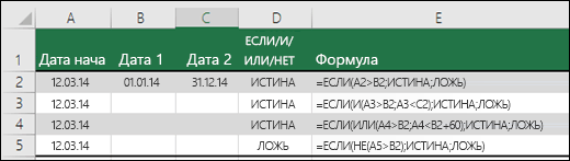
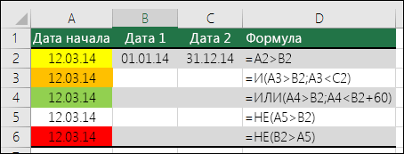
Here are some examples of using AND, OR and NOT to evaluate dates.

Here are the formulas spelled out according to their logic:
IF A2 is greater than B2, return TRUE, otherwise return FALSE. 03/12/14 is greater than 01/01/14, so the formula returns TRUE.
=IF(AND(A3>B2,A3 B2,A4 B2),TRUE,FALSE)
IF A5 is not greater than B2, then return TRUE, otherwise return FALSE. In this case, A5 is greater than B2, so the formula returns FALSE.

Using AND, OR and NOT with Conditional Formatting
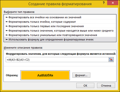
You can also use AND, OR and NOT to set Conditional Formatting criteria with the formula option. When you do this you can omit the IF function and use AND, OR and NOT on their own.
From the Home tab, click Conditional Formatting > New Rule. Next, select the “ Use a formula to determine which cells to format” option, enter your formula and apply the format of your choice.
 Edit Rule dialog showing the Formula method» loading=»lazy»>
Using the earlier Dates example, here is what the formulas would be.

If A2 is greater than B2, format the cell, otherwise do nothing.
=AND(A3>B2,A3 B2,A4 B2)
If A5 is NOT greater than B2, format the cell, otherwise do nothing. In this case A5 is greater than B2, so the result will return FALSE. If you were to change the formula to =NOT(B2>A5) it would return TRUE and the cell would be formatted.
Note: A common error is to enter your formula into Conditional Formatting without the equals sign (=). If you do this you’ll see that the Conditional Formatting dialog will add the equals sign and quotes to the formula — =»OR(A4>B2,A4
Need more help?

See also
You can always ask an expert in the Excel Tech Community or get support in the Answers community.
Источник
Использование ЕСЛИ с функциями И, ИЛИ и НЕ
Функция ЕСЛИ позволяет выполнять логические сравнения значений и ожидаемых результатов. Она проверяет условие и в зависимости от его истинности возвращает результат.
=ЕСЛИ(это истинно, то сделать это, в противном случае сделать что-то еще)
Но что делать, если необходимо проверить несколько условий, где, допустим, все условия должны иметь значение ИСТИНА или ЛОЖЬ ( И), только одно условие должно иметь такое значение ( ИЛИ) или вы хотите убедиться, что данные НЕ соответствуют условию? Эти три функции можно использовать самостоятельно, но они намного чаще встречаются в сочетании с функцией ЕСЛИ.
Используйте функцию ЕСЛИ вместе с функциями И, ИЛИ и НЕ, чтобы оценивать несколько условий.
ЕСЛИ(И()): ЕСЛИ(И(лог_выражение1; [лог_выражение2]; …), значение_если_истина; [значение_если_ложь]))
ЕСЛИ(ИЛИ()): ЕСЛИ(ИЛИ(лог_выражение1; [лог_выражение2]; …), значение_если_истина; [значение_если_ложь]))
ЕСЛИ(НЕ()): ЕСЛИ(НЕ(лог_выражение1), значение_если_истина; [значение_если_ложь]))
Условие, которое нужно проверить.
Значение, которое должно возвращаться, если лог_выражение имеет значение ИСТИНА.
Значение, которое должно возвращаться, если лог_выражение имеет значение ЛОЖЬ.
Общие сведения об использовании этих функций по отдельности см. в следующих статьях: И, ИЛИ, НЕ. При сочетании с оператором ЕСЛИ они расшифровываются следующим образом:
И: =ЕСЛИ(И(условие; другое условие); значение, если ИСТИНА; значение, если ЛОЖЬ)
ИЛИ: =ЕСЛИ(ИЛИ(условие; другое условие); значение, если ИСТИНА; значение, если ЛОЖЬ)
НЕ: =ЕСЛИ(НЕ(условие); значение, если ИСТИНА; значение, если ЛОЖЬ)
Примеры
Ниже приведены примеры распространенных случаев использования вложенных операторов ЕСЛИ(И()), ЕСЛИ(ИЛИ()) и ЕСЛИ(НЕ()). Функции И и ИЛИ поддерживают до 255 отдельных условий, но рекомендуется использовать только несколько условий, так как формулы с большой степенью вложенности сложно создавать, тестировать и изменять. У функции НЕ может быть только одно условие.
Ниже приведены формулы с расшифровкой их логики.
=ЕСЛИ(И(A2>0;B2 0;B4 50);ИСТИНА;ЛОЖЬ)
Если A6 (25) НЕ больше 50, возвращается значение ИСТИНА, в противном случае возвращается значение ЛОЖЬ. В этом случае значение не больше чем 50, поэтому формула возвращает значение ИСТИНА.
Если значение A7 («синий») НЕ равно «красный», возвращается значение ИСТИНА, в противном случае возвращается значение ЛОЖЬ.
Обратите внимание, что во всех примерах есть закрывающая скобка после условий. Аргументы ИСТИНА и ЛОЖЬ относятся ко внешнему оператору ЕСЛИ. Кроме того, вы можете использовать текстовые или числовые значения вместо значений ИСТИНА и ЛОЖЬ, которые возвращаются в примерах.
Вот несколько примеров использования операторов И, ИЛИ и НЕ для оценки дат.
Ниже приведены формулы с расшифровкой их логики.
Если A2 больше B2, возвращается значение ИСТИНА, в противном случае возвращается значение ЛОЖЬ. В этом случае 12.03.14 больше чем 01.01.14, поэтому формула возвращает значение ИСТИНА.
=ЕСЛИ(И(A3>B2;A3 B2;A4 B2);ИСТИНА;ЛОЖЬ)
Если A5 не больше B2, возвращается значение ИСТИНА, в противном случае возвращается значение ЛОЖЬ. В этом случае A5 больше B2, поэтому формула возвращает значение ЛОЖЬ.
Использование операторов И, ИЛИ и НЕ с условным форматированием
Вы также можете использовать операторы И, ИЛИ и НЕ в формулах условного форматирования. При этом вы можете опустить функцию ЕСЛИ.
На вкладке Главная выберите Условное форматирование > Создать правило. Затем выберите параметр Использовать формулу для определения форматируемых ячеек, введите формулу и примените формат.
 «Изменить правило» с параметром «Формула»» loading=»lazy»>
Вот как будут выглядеть формулы для примеров с датами:
Если A2 больше B2, отформатировать ячейку, в противном случае не выполнять никаких действий.
=И(A3>B2;A3 B2;A4 B2)
Если A5 НЕ больше B2, отформатировать ячейку, в противном случае не выполнять никаких действий. В этом случае A5 больше B2, поэтому формула возвращает значение ЛОЖЬ. Если изменить формулу на =НЕ(B2>A5), она вернет значение ИСТИНА, а ячейка будет отформатирована.
Примечание: Распространенной ошибкой является ввод формулы в условное форматирование без знака равенства (=). В этом случае вы увидите, что диалоговое окно Условное форматирование добавит знак равенства и кавычки в формулу — =»OR(A4>B2,A4
Дополнительные сведения

См. также
Вы всегда можете задать вопрос специалисту Excel Tech Community или попросить помощи в сообществе Answers community.
Источник
AND function
Use the AND function, one of the logical functions, to determine if all conditions in a test are TRUE.
Example
The AND function returns TRUE if all its arguments evaluate to TRUE, and returns FALSE if one or more arguments evaluate to FALSE.
One common use for the AND function is to expand the usefulness of other functions that perform logical tests. For example, the IF function performs a logical test and then returns one value if the test evaluates to TRUE and another value if the test evaluates to FALSE. By using the AND function as the logical_test argument of the IF function, you can test many different conditions instead of just one.
The AND function syntax has the following arguments:
Required. The first condition that you want to test that can evaluate to either TRUE or FALSE.
Optional. Additional conditions that you want to test that can evaluate to either TRUE or FALSE, up to a maximum of 255 conditions.
The arguments must evaluate to logical values, such as TRUE or FALSE, or the arguments must be arrays or references that contain logical values.
If an array or reference argument contains text or empty cells, those values are ignored.
If the specified range contains no logical values, the AND function returns the #VALUE! error.
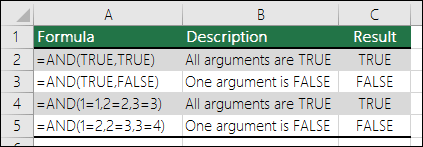
Examples
Here are some general examples of using AND by itself, and in conjunction with the IF function.
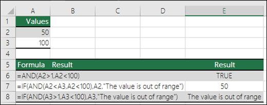
=AND(A2>1,A2 AND less than 100, otherwise it displays FALSE.
Displays the value in cell A2 if it’s less than A3 AND less than 100, otherwise it displays the message «The value is out of range».
=IF(AND(A3>1,A3 AND less than 100, otherwise it displays a message. You can substitute any message of your choice.
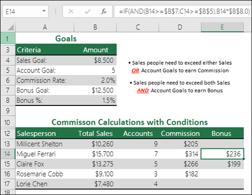
Here is a fairly common scenario where we need to calculate if sales people qualify for a bonus using IF and AND.
 =$B$7,C14>=$B$5),B14*$B$8,0)» loading=»lazy»>
=IF(AND(B14>=$B$7,C14>=$B$5),B14*$B$8,0) – IF Total Sales are greater than or equal (>=) to the Sales Goal, AND Accounts are greater than or equal to (>=) the Account Goal, then multiply Total Sales by the Bonus %, otherwise return 0.
Need more help?
You can always ask an expert in the Excel Tech Community or get support in the Answers community.
Источник
How to use Conditional Formatting

Conditional formatting is a data visualization tool in several spreadsheet applications. We use it to highlight, emphasize, and differentiate by using colors or other means (like applying icons) to cells or ranges relevant to us.
At first, you will learn the essential skills. The second part of the tutorial will be about using Excel conditional formatting formulas and examples.
Table of contents:
What is Conditional Formatting
Conditional formatting offers a wide range of possibilities for Excel users. Its first and foremost function is to direct attention to the most crucial data points. Then, we can determine with rules what are the most important for us. These data points can be deadlines, excellent sales results, or tasks carrying a high risk.
Fundamentals of Conditional Formatting
Before we walk you through all possibilities of conditional formatting, we have to stall a bit. It is necessary to know all the basics! First, you have to understand the structure that conditional formatting provides. So, let’s see a little overview. In short, we will summarize the most important rules for you.
Logical Operators (if-then rules): Every single conditional formatting rule is based on straightforward logic. If “X” criteria are true, then apply the rule “Y”. Let’s see a simple example: “X” criteria are: “The sales price is more than $50.” “Y” criteria are defined as a color all applicable cells red. What will happen now? By applying the if-then rule, every cell will be colored red where the sales price is > $50, more than $50.
Predefined Conditions (built-in presets): This option can interest beginners. In Excel, there are many built-in rules and conditions available. We have also thought about users with different capabilities when making the tutorial. We will learn about this subject from a detailed guide.
User-defined Conditions: There are often situations when the default settings are unsuitable for the given task. No problem, let’s make our own rules. Use the Excel formulas so we can reach the required results. We have to note that we can use all of the formulas in Excel to create the rules.
Multiple Conditions: We can simultaneously apply multiple rules for one cell or range. If there are more rules active simultaneously, which one will prevail? We will discuss this in detail in the chapter “rule hierarchy and precedence.”
Highlight Cells using rules (if the quantity is greater than 200)
Click the Highlight Cells Rules functions to highlight patterns and trends with conditional formatting. It will be straightforward to identify the cells that meet your criteria. This is a basic color formatting method for cells and ranges.
Select the range you want to use a rule and apply highlight rules. In our example, we will highlight any product that’s quantity is greater than 200 units. For example, select the range’ H2: H24′.
In the Home tab of the ribbon, click Conditional Formatting, then click Highlight Cell Rules. Finally, select ‘Greater than’.
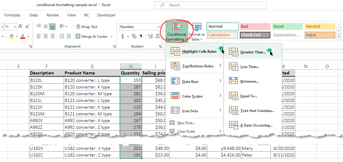
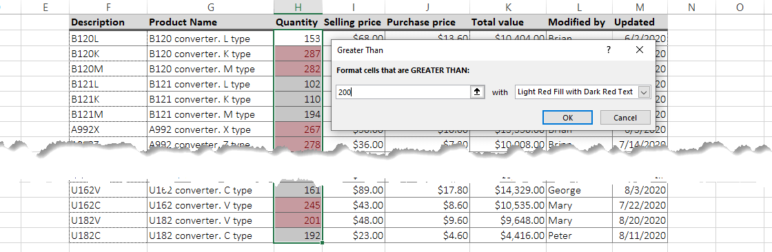
Now, a dialog box will appear. Enter 200 In the left box. So, if you enter 200, something will happen when the value is greater than 200. But what will happen? You will define the trigger in the right box.
Explanation: Triggers can be defined in the range with which the event is associated. Just forget the standard option and select a light red fill from the drop-down list. If you click OK now, all the cells that are above 200 will be formatted based on the given rule.
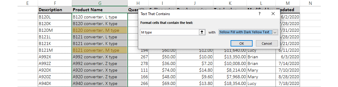
Highlight cells that contain text
If you are looking for all the M types of converters in column G, you do not have to scan the screen for hours and hours. Instead, you can let conditional formatting do all the dirty work and highlight the criteria easily and automatically.
Select the range with text. In this example, you will select the range G2:G24, all our ‘Product Name.’
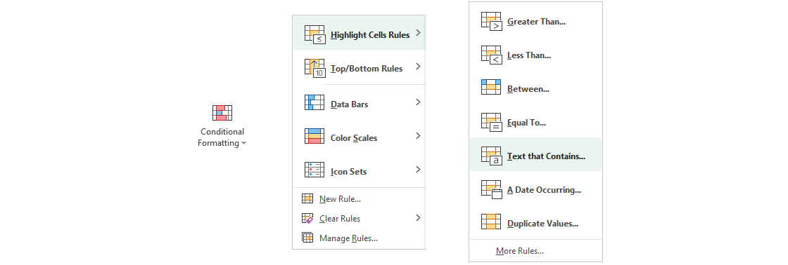
Click Conditional Formatting, hover the mouse over Highlight Cells Rules, and choose Text that Contains.
Enter “M type” in the text box. Next, select yellow fill color with dark yellow text using the drop-down menu, then click OK.
Tip: You can apply a custom format if the default style is unsuitable. Use the drop-down menu and select the Custom format option to create your format. You can create custom styles by changing the font, border, or fill types. Keep in mind the basics of conditional formatting! Further options are available if you can apply different rules. You can also use important highlight rules for your values: Greater than…, Equal to…, or Between.
Editing a conditional formatting rule
This section will show you how to manage conditional formatting rules. You can modify the selected rule using the conditional formatting rules manager. Use this function if you want to edit some of these rules later or delete them.
This function can be accessed using the Home Tab and the Conditional Formatting button. Then select Manage Rules from the drop-down list. By default, you’ll see a dialog box:
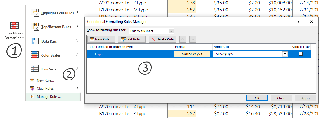
By default, the “Show formatting rules for:” is set to “Current Selection”. Next, select the “This Worksheet” option from the drop-down list to display the conditional formatting rules you have applied to the actual Worksheet.
Use top-bottom rules and select the rule from the list you want to modify. Then, click the rule you want to change to edit a rule. In this example, we want to highlight the top 10 values in the Total value column. Currently, the top five are highlighted.
Click the Top 5 rows! Excel highlights the selected rows with blue. Then, click Edit Rule. A dialog box opens where you can change the given conditions of the rule; type 10 in the number field. Finally, click OK.

We’ll get the Manage Rules box back. Click OK to save the changes.
Delete a conditional formatting rule
Sometimes your spreadsheet looks like a traffic jam regarding too many conditional formatting rules. This is because Excel has a hidden “feature.” If you have many unique rules, that may be the reason for the slow calculations. In this case, you should eliminate some rules in the sheet.
Tip: Excel provides a quick way to delete rules. Click the Conditional Formatting button on the Home tab and select clear rules.

But it’s not smart to delete all rules from a worksheet!
In this case, we would like to delete the rules from Column G (Product Names). Select the ‘G2:G24’ range.
To properly delete a rule, select the ‘Manage Rules’ box and click on the conditional formatting rule you want to remove.
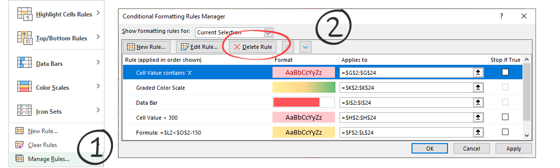
Click OK to delete the rule.
We hope you have found the first part of the tutorial interesting and exciting. In this, we have introduced how we can use the basic rules with Excel.
Conditional Formatting and Formulas
You’ll find here 50+ formula examples and learn more about custom formulas.
All examples are based on a few simple steps:
- Select the range that you want to apply the format
- Add ‘New Rule’
- Enter the formula
- Select format style
- Click ‘OK, then click ‘Apply.’
Check our definitive guide with examples if you want to learn about Excel Formulas.
How do I highlight the lowest 3 values in Excel?
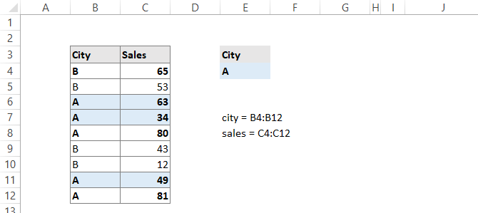
Create a formula to determine the 3 smallest values that meet specific criteria. Use a formula based on the AND and SMALL functions. In the example, the formula used for conditional formatting is:
where “city” is the named range B4:B12, and “sales” is the named range C4:C12.
How to conditional format if the cell is blank?
![]()
In the following example, you want to highlight values in one column when values in one or more columns are blank. A basic formula based on the OR and ISBLANK functions is used to test for blank or empty cells. For example, if any cell in a corresponding row in the range B4:E12 is blank, OR function returns TRUE. Thus, the trigger will be fired, and the cell in column F will highlight using light blue.
Use the conditional formatting formula:
How to use Conditional Formatting to highlight past due dates in Excel
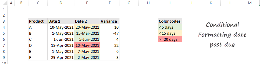
You will apply a formula in the example to determine “past due dates.” The formula will check if the variance between dates is greater than a certain number of days. To create a color-coded table, use three conditional formatting rules for each interval.
Select the cells in range E4:E9 and apply the formulas.
- =(E4-D4) =20 if the difference between the two dates is greater than or equal to 20
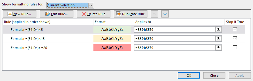
Important: You have to use the stop-if-true checkbox for rule1 and rule2.
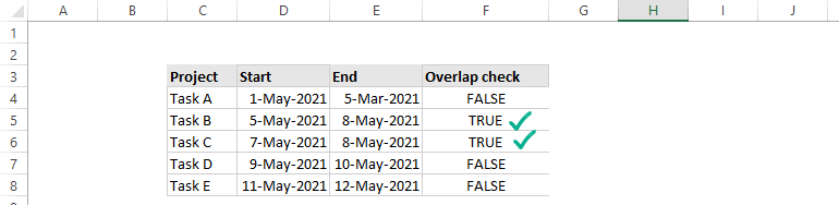
How to highlight overlapping dates in Excel
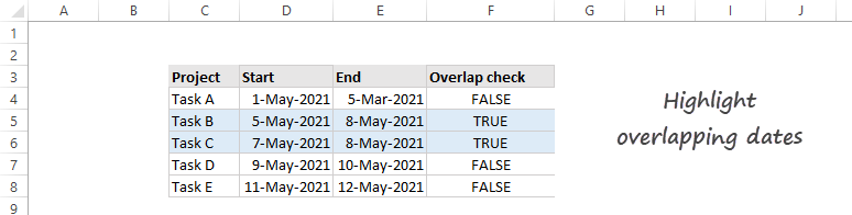
Sometimes you need to highlight cells where dates overlap. You can use conditional formatting formulas and apply the SUMPRODUCT function in the example. What are overlapping dates? We are talking about overlapping dates if these two conditions are true:
- First, the start date is less than equal to the other end dates in the column.
- The end date is greater than or equal to at least one other start date.
Create a new column to check the conditions. Then, apply the formula to cell F4 them copy the formula down.
Now create a conditional formatting rule. First, select the cells you want to format, in this case, range C4:F8. Then use the rule below to highlight overlapping dates.
So, click OK to apply the rule. If the result is TRUE, the given row cells in the selection will be highlighted.
Final thought
Finally, take a closer look at the advanced conditional formatting rules:
- You should know how the conditional formatting rule hierarchy works if you work with multiple rules.
- The Stop if True tool helps you to manage overlaps between rules.
- Color ranking helps you identify the maximum value in a range and highlight them.
- Learn how to use Multiple Conditions and Formulas.
Conditional formatting makes our lives in Excel a lot easier.
Use formulas wisely! We can highlight all the key information that fits the criteria. Knowing and applying conditional formatting rules decrease the time spent on data analysis. Therefore, we can be a lot more productive. We can effectively support company decisions by recognizing the patterns (whether positive or negative). Look at the in-depth article called ‘How to create an Excel Dashboard‘ regarding conditional formatting on our blog.
Additional resources
Ultimate Dashboard Tools
Pro Dashboard Add-in for Excel. Fully automated. Lightweight. No coding skills required.
Источник
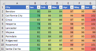
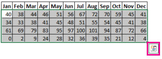
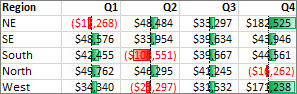
Conditional formatting can help make patterns and trends in your data more apparent. To use it, you create rules that determine the format of cells based on their values, such as the following monthly temperature data with cell colors tied to cell values.
You can apply conditional formatting to a range of cells (either a selection or a named range), an Excel table, and in Excel for Windows, even a PivotTable report.

Conditional formatting typically works the same way in a range of cells, an Excel table, or a PivotTable report. However, conditional formatting in a PivotTable report has some extra considerations:
-
There are some conditional formats that don’t work with fields in the Values area of a PivotTable report. For example, you can’t format such fields based on whether they contain unique or duplicate values. These restrictions are mentioned in the remaining sections of this article, where applicable.
-
If you change the layout of the PivotTable report by filtering, hiding levels, collapsing and expanding levels, or moving a field, the conditional format is maintained as long as the fields in the underlying data are not removed.
-
The scope of the conditional format for fields in the Values area can be based on the data hierarchy and is determined by all the visible children (the next lower level in a hierarchy) of a parent (the next higher level in a hierarchy) on rows for one or more columns, or columns for one or more rows.
Note: In the data hierarchy, children do not inherit conditional formatting from the parent, and the parent does not inherit conditional formatting from the children.
-
There are three methods for scoping the conditional format of fields in the Values area: by selection, by corresponding field, and by value field.
The default method of scoping fields in the Values area is by selection. You can change the scoping method to the corresponding field or value field by using the Apply formatting rule to option button, the New Formatting Rule dialog box, or the Edit Formatting Rule dialog box.
|
Method |
Use this method if you want to select |
|
Scoping by selection |
|
|
Scoping by value field |
|
|
Scoping by corresponding field |
When you conditionally format fields in the Values area for top, bottom, above average, or below average values, the rule is based on all visible values by default. However, when you scope by corresponding field, instead of using all visible values, you can apply the conditional format for each combination of:
|
Note: Quick Analysis is not available in Excel 2010 and previous versions.
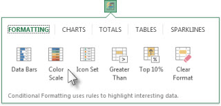
Use the Quick Analysis button  to apply selected conditional formatting to the selected data. The Quick Analysis button appears automatically when you select data.
-
Select the data that you want to conditionally format. The Quick Analysis button appears on the lower-right corner of the selection.

-
Click the Quick Analysis button
, or press Ctrl+Q. -
In the pop-up that appears, on the Formatting tab, move your mouse over the different options to see a Live Preview on your data, and then click on the formatting option you want.
Notes:
-
The formatting options that appear in the Formatting tab depend on the data you have selected. If your selection contains only text, then the available options are Text, Duplicate, Unique, Equal To, and Clear. When the selection contains only numbers, or both text and numbers, then the options are Data Bars, Colors, Icon Sets, Greater, Top 10%, and Clear.
-
Live preview will only render for those formatting options that can be used on your data. For example, if your selected cells don’t contain matching data and you select Duplicate, the live preview will not work.
-
-
If the Text that Contains dialog box appears, enter the formatting option you want to apply and click OK.
If you’d like to watch a video that shows how to use Quick Analysis to apply conditional formatting, see Video: Use conditional formatting.
You can download a sample workbook that contains different examples of applying conditional formatting, both with standard rules such as top and bottom, duplicates, Data Bars, Icon Sets and Color Scales, as well as manually creating rules of your own.
Download: Conditional formatting examples in Excel
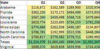
Color scales are visual guides that help you understand data distribution and variation. A two-color scale helps you compare a range of cells by using a gradation of two colors. The shade of the color represents higher or lower values. For example, in a green and yellow color scale, as shown below, you can specify that higher value cells have a more green color and lower value cells have a more yellow color.
Tip: You can sort cells that have this format by their color — just use the context menu.
Tip: If any cells in the selection contain a formula that returns an error, the conditional formatting is not applied to those cells. To ensure that the conditional formatting is applied to those cells, use an IS or IFERROR function to return a value other than an error value.
Quick formatting
-
Select one or more cells in a range, table, or PivotTable report.
-
On the Home tab, in the Styles group, click the arrow next to Conditional Formatting, and then click Color Scales.
-
Select a two-color scale.
Hover over the color scale icons to see which icon is a two-color scale. The top color represents higher values, and the bottom color represents lower values.
You can change the method of scoping for fields in the Values area of a PivotTable report by using the Formatting Options button that appears next to a PivotTable field that has conditional formatting applied.
Advanced formatting
-
Select one or more cells in a range, table, or PivotTable report.
-
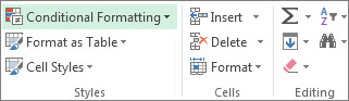
On the Home tab, in the Styles group, click the arrow next to Conditional Formatting, and then click Manage Rules. The Conditional Formatting Rules Manager dialog box appears.
-
Do one of the following:
-
To add a completely new conditional format, click New Rule. The New Formatting Rule dialog box appears.
-
To add a new conditional format based on one that is already listed, select the rule, then click Duplicate Rule. The duplicate rule appears in the dialog box. Select the duplicate, then select Edit Rule. The Edit Formatting Rule dialog box appears.
-
To change a conditional format, do the following:
-
Make sure that the appropriate worksheet, table, or PivotTable report is selected in the Show formatting rules for list box.
-
Optionally, change the range of cells by clicking Collapse Dialog in the Applies to box to temporarily hide the dialog box, by selecting the new range of cells on the worksheet, and then by selecting Expand Dialog.
-
Select the rule, and then click Edit rule. The Edit Formatting Rule dialog box appears.
-
-
-
Under Apply Rule To, to optionally change the scope for fields in the Values area of a PivotTable report by:
-
Selection: Click Selected cells.
-
All cells for a Value label: Click All cells showing <Value label> values.
-
All cells for a Value label, excluding subtotals and the grand total: Click All cells showing <Value label> values for <Row Label>.
-
-
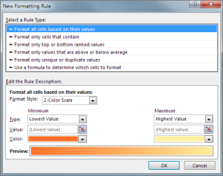
Under Select a Rule Type, click Format all cells based on their values (default).
-
Under Edit the Rule Description, in the Format Style list box, select 2-Color Scale.
-
To select a type in the Type box for Minimum and Maximum, do one of the following:
-
Format lowest and highest values: Select Lowest Value and Highest Value.
In this case, you do not enter a Minimum and MaximumValue.
-
Format a number, date, or time value: Select Number and then enter a Minimum and MaximumValue.
-
Format a percentage Percent: Enter a Minimum and MaximumValue.
Valid values are from 0 (zero) to 100. Don’t enter a percent sign.
Use a percentage when you want to visualize all values proportionally because the distribution of values is proportional.
-
Format a percentile: Select Percentile and then enter a Minimum and MaximumValue. Valid percentiles are from 0 (zero) to 100.
Use a percentile when you want to visualize a group of high values (such as the top 20thpercentile) in one color grade proportion and low values (such as the bottom 20th percentile) in another color grade proportion, because they represent extreme values that might skew the visualization of your data.
-
Format a formula result: Select Formula and then enter values for Minimum and Maximum.
-
The formula must return a number, date, or time value.
-
Start the formula with an equal sign (=).
-
Invalid formulas result in no formatting being applied.
-
It’s a good idea to test the formula to make sure that it doesn’t return an error value.
Notes:
-
Make sure that the Minimum value is less than the Maximum value.
-
You can choose a different type for the Minimum and Maximum. For example, you can choose a number for Minimum a percentage for Maximum.
-
-
-
-
To choose a Minimum and Maximum color scale, click Color for each, and then select a color.
If you want to choose additional colors or create a custom color, click More Colors. The color scale you select is shown in the Preview box.

Color scales are visual guides that help you understand data distribution and variation. A three-color scale helps you compare a range of cells by using a gradation of three colors. The shade of the color represents higher, middle, or lower values. For example, in a green, yellow, and red color scale, you can specify that higher value cells have a green color, middle value cells have a yellow color, and lower value cells have a red color.
Tip: You can sort cells that have this format by their color — just use the context menu.
Quick formatting
-
Select one or more cells in a range, table, or PivotTable report.
-
On the Home tab, in the Styles group, click the arrow next to Conditional Formatting, and then click Color Scales.
-
Select a three-color scale. The top color represents higher values, the center color represents middle values, and the bottom color represents lower values.
Hover over the color scale icons to see which icon is a three-color scale.
You can change the method of scoping for fields in the Values area of a PivotTable report by using the Formatting Options button that appears next to a PivotTable field that has conditional formatting applied..
Advanced formatting
-
Select one or more cells in a range, table, or PivotTable report.
-
On the Home tab, in the Styles group, click the arrow next to Conditional Formatting, and then click Manage Rules. The Conditional Formatting Rules Manager dialog box appears.
-
Do one of the following:
-
To add a new conditional format, click New Rule. The New Formatting Rule dialog box appears.
-
To add a new conditional format based on one that is already listed, select the rule, then click Duplicate Rule. The duplicate rule is copied and appears in the dialog box. Select the duplicate, then select Edit Rule. The Edit Formatting Rule dialog box appears.
-
To change a conditional format, do the following:
-
Make sure that the appropriate worksheet, table, or PivotTable report is selected in the Show formatting rules for list box.
-
Optionally, change the range of cells by clicking Collapse Dialog in the Applies to box to temporarily hide the dialog box, by selecting the new range of cells on the worksheet, and then by selecting Expand Dialog.
-
Select the rule, and then click Edit rule. The Edit Formatting Rule dialog box appears.
-
-
-
Under Apply Rule To, to optionally change the scope for fields in the Values area of a PivotTable report by:
-
Selection: Click Just these cells.
-
Corresponding field: Click All <value field> cells with the same fields.
-
Value field: Click All <value field> cells.
-
-
Under Select a Rule Type, click Format all cells based on their values.
-
Under Edit the Rule Description, in the Format Style list box, select 3-Color Scale.
-
Select a type for Minimum, Midpoint, and Maximum. Do one of the following:
-
Format lowest and highest values: Select a Midpoint.
In this case, you do not enter a Lowest and HighestValue.
-
Format a number, date, or time value: Select Number and then enter a value for Minimum, Midpoint, and Maximum.
-
Format a percentage: Select Percent and then enter a value for Minimum, Midpoint, and Maximum. Valid values are from 0 (zero) to 100. Do not enter a percent (%) sign.
Use a percentage when you want to visualize all values proportionally, because using a percentage ensures that the distribution of values is proportional.
-
Format a percentile: Select Percentile and then enter a value for Minimum, Midpoint, and Maximum.
Valid percentiles are from 0 (zero) to 100.
Use a percentile when you want to visualize a group of high values (such as the top 20th percentile) in one color grade proportion and low values (such as the bottom 20th percentile) in another color grade proportion, because they represent extreme values that might skew the visualization of your data.
-
Format a formula result: Select Formula and then enter a value for Minimum, Midpoint, and Maximum.
The formula must return a number, date, or time value. Start the formula with an equal sign (=). Invalid formulas result in no formatting being applied. It’s a good idea to test the formula to make sure that it doesn’t return an error value.
Notes:
-
You can set minimum, midpoint, and maximum values for the range of cells. Make sure that the value in Minimum is less than the value in Midpoint, which in turn is less than the value in Maximum.
-
You can choose a different type for Minimum, Midpoint, and Maximum. For example, you can choose a Minimum number, Midpoint percentile, and Maximum percent.
-
In many cases, the default Midpoint value of 50 percent works best, but you can adjust this to fit unique requirements.
-
-
-
To choose a Minimum, Midpoint, and Maximum color scale, click Color for each, and then select a color.
-
To choose additional colors or create a custom color, click More Colors.
-
The color scale you select is shown in the Preview box.
-
A data bar helps you see the value of a cell relative to other cells. The length of the data bar represents the value in the cell. A longer bar represents a higher value, and a shorter bar represents a lower value. Data bars are useful in spotting higher and lower numbers, especially with large amounts of data, such as top selling and bottom selling toys in a holiday sales report.
The example shown here uses data bars to highlight dramatic positive and negative values. You can format data bars so that the data bar starts in the middle of the cell, and stretches to the left for negative values.
Tip: If any cells in the range contain a formula that returns an error, the conditional formatting is not applied to those cells. To ensure that the conditional formatting is applied to those cells, use an IS or IFERROR function to return a value (such as 0 or «N/A») instead of an error value.
Quick formatting
-
Select one or more cells in a range, table, or PivotTable report.
-
On the Home tab, in the Style group, click the arrow next to Conditional Formatting, click Data Bars, and then select a data bar icon.
You can change the method of scoping for fields in the Values area of a PivotTable report by using the Apply formatting rule to option button.
Advanced formatting
-
Select one or more cells in a range, table, or PivotTable report.
-
On the Home tab, in the Styles group, click the arrow next to Conditional Formatting, and then click Manage Rules. The Conditional Formatting Rules Manager dialog box appears.
-
Do one of the following:
-
To add a conditional format, click New Rule. The New Formatting Rule dialog box appears.
-
To add a new conditional format based on one that is already listed, select the rule, then click Duplicate Rule. The duplicate rule is copied and appears in the dialog box. Select the duplicate, then select Edit Rule. The Edit Formatting Rule dialog box appears.
-
To change a conditional format, do the following:
-
-
Make sure that the appropriate worksheet, table, or PivotTable report is selected in the Show formatting rules for list box.
-
Optionally, change the range of cells by clicking Collapse Dialog in the Applies to box to temporarily hide the dialog box, by selecting the new range of cells on the worksheet, and then by selecting Expand Dialog.
-
Select the rule, and then click Edit rule. The Edit Formatting Rule dialog box appears.
-
-
-
Under Apply Rule To, to optionally change the scope for fields in the Values area of a PivotTable report by:
-
Selection: Click Just these cells.
-
Corresponding field: Click All <value field> cells with the same fields.
-
Value field: Click All <value field> cells.
-
-
Under Select a Rule Type, click Format all cells based on their values.
-
Under Edit the Rule Description, in the Format Style list box, select Data Bar.
-
Select a Minimum and MaximumType. Do one of the following:
-
Format lowest and highest values: Select Lowest Value and Highest Value.
In this case, you do not enter a value for Minimum and Maximum.
-
Format a number, date, or time value: Select Number and then enter a Minimum and MaximumValue.
-
Format a percentage: Select Percent and then enter a value for Minimum and Maximum.
Valid values are from 0 (zero) to 100. Do not enter a percent (%) sign.
Use a percentage when you want to visualize all values proportionally, because using a percentage ensures that the distribution of values is proportional.
-
Format a percentile Select Percentile and then enter a value for Minimum and Maximum.
Valid percentiles are from 0 (zero) to 100.
Use a percentile when you want to visualize a group of high values (such as the top 20th percentile) in one data bar proportion and low values (such as the bottom 20th percentile) in another data bar proportion, because they represent extreme values that might skew the visualization of your data.
-
Format a formula result Select Formula, and then enter a value for Minimum and Maximum.
-
The formula has to return a number, date, or time value.
-
Start the formula with an equal sign (=).
-
Invalid formulas result in no formatting being applied.
-
It’s a good idea to test the formula to make sure that it doesn’t return an error value.
-
Notes:
-
Make sure that the Minimum value is less than the Maximum value.
-
You can choose a different type for Minimum and Maximum. For example, you can choose a Minimum number and a Maximum percent.
-
-
To choose a Minimum and Maximum color scale, click Bar Color.
If you want to choose additional colors or create a custom color, click More Colors. The bar color you select is shown in the Preview box.
-
To show only the data bar and not the value in the cell, select Show Bar Only.
-
To apply a solid border to data bars, select Solid Border in the Border list box and choose a color for the border.
-
To choose between a solid bar and a gradiated bar, choose Solid Fill or Gradient Fill in the Fill list box.
-
To format negative bars, click Negative Value and Axis and then, in the Negative Value and Axis Settings dialog box, choose options for the negative bar fill and border colors. You can choose position settings and a color for the axis. When you are finished selecting options, click OK.
-
You can change the direction of bars by choosing a setting in the Bar Direction list box. This is set to Context by default, but you can choose between a left-to-right and a right-to-left direction, depending on how you want to present your data.
Use an icon set to annotate and classify data into three to five categories separated by a threshold value. Each icon represents a range of values. For example, in the 3 Arrows icon set, the green up arrow represents higher values, the yellow sideways arrow represents middle values, and the red down arrow represents lower values.
Tip: You can sort cells that have this format by their icon — just use the context menu.
The example shown here works with several examples of conditional formatting icon sets.

You can choose to show icons only for cells that meet a condition; for example, displaying a warning icon for those cells that fall below a critical value and no icons for those that exceed it. To do this, you hide icons by selecting No Cell Icon from the icon drop-down list next to the icon when you are setting conditions. You can also create your own combination of icon sets; for example, a green «symbol» check mark, a yellow «traffic light», and a red «flag.»
Tip: If any cells in the selection contain a formula that returns an error, the conditional formatting is not applied to those cells. To ensure that the conditional formatting is applied to those cells, use an IS or IFERROR function to return a value (such as 0 or «N/A») instead of an error value.
Quick formatting
-
Select the cells that you want to conditionally format.
-
On the Home tab, in the Style group, click the arrow next to Conditional Formatting, click Icon Set, and then select an icon set.
You can change the method of scoping for fields in the Values area of a PivotTable report by using the Apply formatting rule to option button.
Advanced formatting
-
Select the cells that you want to conditionally format.
-
On the Home tab, in the Styles group, click the arrow next to Conditional Formatting, and then click Manage Rules. The Conditional Formatting Rules Manager dialog box appears.
-
Do one of the following:
-
To add a conditional format, click New Rule. The New Formatting Rule dialog box appears.
-
To add a new conditional format based on one that is already listed, select the rule, then click Duplicate Rule. The duplicate rule is copied and appears in the dialog box. Select the duplicate, then select Edit Rule. The Edit Formatting Rule dialog box appears.
-
To change a conditional format, do the following:
-
Make sure that the appropriate worksheet, table, or PivotTable report is selected in the Show formatting rules for list box.
-
Optionally, change the range of cells by clicking Collapse Dialog in the Applies to box to temporarily hide the dialog box, by selecting the new range of cells on the worksheet, and then by selecting Expand Dialog.
-
Select the rule, and then click Edit rule. The Edit Formatting Rule dialog box appears.
-
-
-
Under Apply Rule To, to optionally change the scope for fields in the Values area of a PivotTable report by:
-
Selection: Click Just these cells.
-
Corresponding field: Click All <value field> cells with the same fields.
-
Value field: Click All <value field> cells.
-
-
Under Select a Rule Type, click Format all cells based on their values.
-
Under Edit the Rule Description, in the Format Style list box, select Icon Set.
-
Select an icon set. The default is 3 Traffic Lights (Unrimmed). The number of icons and the default comparison operators and threshold values for each icon can vary for each icon set.
-
You can adjust the comparison operators and threshold values. The default range of values for each icon are equal in size, but you can adjust these to fit your unique requirements. Make sure that the thresholds are in a logical sequence of highest to lowest from top to bottom.
-
Do one of the following:
-
Format a number, date, or time value: Select Number.
-
Format a percentage: Select Percent.
Valid values are from 0 (zero) to 100. Do not enter a percent (%) sign.
Use a percentage when you want to visualize all values proportionally, because using a percentage ensures that the distribution of values is proportional.
-
Format a percentile: Select Percentile. Valid percentiles are from 0 (zero) to 100.
Use a percentile when you want to visualize a group of high values (such as the top 20th percentile) using a particular icon and low values (such as the bottom 20th percentile) using another icon, because they represent extreme values that might skew the visualization of your data.
-
Format a formula result: Select Formula, and then enter a formula in each Value box.
-
The formula must return a number, date, or time value.
-
Start the formula with an equal sign (=).
-
Invalid formulas result in no formatting being applied.
-
It’s a good idea to test the formula to make sure that it doesn’t return an error value.
-
-
-
To make the first icon represent lower values and the last icon represent higher values, select Reverse Icon Order.
-
To show only the icon and not the value in the cell, select Show Icon Only.
Notes:
-
You may need to adjust the column width to accommodate the icon.
-
The size of the icon shown depends on the font size that is used in that cell. As the size of the font is increased, the size of the icon increases proportionally.
-
-
To more easily find specific cells, you can format them by using a comparison operator. For example, in an inventory worksheet sorted by categories, you could highlight products with fewer than 10 items on hand in yellow. Or, in a retail store summary worksheet, you might identify all stores with profits greater than 10%, sales volumes less than $100,000, and region equal to «SouthEast.»
The examples shown here work with examples of built-in conditional formatting criteria, such as Greater Than, and Top %. This formats cities with a population greater than 2,000,000 with a green background and average high temperatures in the top 30% with orange.
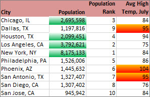
Note: You cannot conditionally format fields in the Values area of a PivotTable report by text or by date, only by number.
Quick formatting
-
Select one or more cells in a range, table, or PivotTable report.
-
On the Home tab, in the Style group, click the arrow next to Conditional Formatting, and then click Highlight Cells Rules.
-
Select the command you want, such as Between, Equal To Text that Contains, or A Date Occurring.
-
Enter the values you want to use, and then select a format.
You can change the method of scoping for fields in the Values area of a PivotTable report by using the Apply formatting rule to option button.
If you’d like to watch videos of these techniques, see Video: Conditionally format text and Video: Conditionally format dates.
Advanced formatting
-
Select one or more cells in a range, table, or PivotTable report.
-
On the Home tab, in the Styles group, click the arrow next to Conditional Formatting, and then click Manage Rules. The Conditional Formatting Rules Manager dialog box appears.
-
Do one of the following:
-
To add a conditional format, click New Rule. The New Formatting Rule dialog box appears.
-
To add a new conditional format based on one that is already listed, select the rule, then click Duplicate Rule. The duplicate rule is copied and appears in the dialog box. Select the duplicate, then select Edit Rule. The Edit Formatting Rule dialog box appears.
-
To change a conditional format, do the following:
-
-
Make sure that the appropriate worksheet, table, or PivotTable report is selected in the Show formatting rules for list box.
-
Optionally, change the range of cells by clicking Collapse Dialog in the Applies to box to temporarily hide the dialog box, by selecting the new range of cells on the worksheet or on other worksheets, and then by selecting Expand Dialog.
-
Select the rule, and then click Edit rule. The Edit Formatting Rule dialog box appears.
-
-
-
Under Apply Rule To, to optionally change the scope for fields in the Values area of a PivotTable report by:
-
Selection: Click Just these cells.
-
Corresponding field: Click All <value field> cells with the same fields.
-
Value field: Click All <value field> cells.
-
-
Under Select a Rule Type, click Format only cells that contain.
-
Under Edit the Rule Description, in the Format only cells with list box, do one of the following:
-
Format by number, date, or time: Select Cell Value, select a comparison operator, and then enter a number, date, or time.
For example, select Between and then enter 100 and 200, or select Equal to and then enter 1/1/2009.
You can also enter a formula that returns a number, date, or time value.
-
If you enter a formula, start it with an equal sign (=).
-
Invalid formulas result in no formatting being applied.
-
It’s a good idea to test the formula to make sure that it doesn’t return an error value.
-
-
Format by text: Select Specific Text, choosing a comparison operator, and then enter text.
For example, select Contains and then enter Silver, or select Starting with and then enter Tri.
Quotes are included in the search string, and you may use wildcard characters. The maximum length of a string is 255 characters.
You can also enter a formula that returns text.
-
If you enter a formula, start it with an equal sign (=).
-
Invalid formulas result in no formatting being applied.
-
It’s a good idea to test the formula to make sure that it doesn’t return an error value.
To see a video of this technique, see Video: Conditionally format text.
-
-
Format by date: Select Dates Occurring and then select a date comparison.
For example, select Yesterday or Next week.
To see a video of this technique, see Video: Conditionally format dates.
-
Format cells with blanks or no blanks: Select Blanks or No Blanks.
A blank value is a cell that contains no data and is different from a cell that contains one or more spaces (spaces are considered as text).
-
Format cells with error or no error values: Select Errors or No Errors.
Error values include: #####, #VALUE!, #DIV/0!, #NAME?, #N/A, #REF!, #NUM!, and #NULL!.
-
-
To specify a format, click Format. The Format Cells dialog box appears.
-
Select the number, font, border, or fill format you want to apply when the cell value meets the condition, and then click OK.
You can choose more than one format. The formats you select are shown in the Preview box.
You can find the highest and lowest values in a range of cells that are based on a cutoff value you specify. For example, you can find the top 5 selling products in a regional report, the bottom 15% products in a customer survey, or the top 25 salaries in a department .
Quick formatting
-
Select one or more cells in a range, table, or PivotTable report.
-
On the Home tab, in the Style group, click the arrow next to Conditional Formatting, and then click Top/Bottom Rules.
-
Select the command you want, such as Top 10 items or Bottom 10 %.
-
Enter the values you want to use, and then select a format.
You can change the method of scoping for fields in the Values area of a PivotTable report by using the Apply formatting rule to option button.
Advanced formatting
-
Select one or more cells in a range, table, or PivotTable report.
-
On the Home tab, in the Styles group, click the arrow next to Conditional Formatting, and then click Manage Rules. The Conditional Formatting Rules Manager dialog box appears.
-
Do one of the following:
-
To add a conditional format, click New Rule. The New Formatting Rule dialog box appears.
-
To add a new conditional format based on one that is already listed, select the rule, then click Duplicate Rule. The duplicate rule is copied and appears in the dialog box. Select the duplicate, then select Edit Rule. The Edit Formatting Rule dialog box appears.
-
To change a conditional format, do the following:
-
-
Make sure that the appropriate worksheet, table, or PivotTable report is selected in the Show formatting rules for list box.
-
Optionally, change the range of cells by clicking Collapse Dialog in the Applies to box to temporarily hide the dialog box, by selecting the new range of cells on the worksheet, and then by selecting Expand Dialog.
-
Select the rule, and then click Edit rule. The Edit Formatting Rule dialog box appears.
-
-
-
Under Apply Rule To, to optionally change the scope fields in the Values area of a PivotTable report by:
-
Selection: Click Just these cells.
-
Corresponding field: Click All <value field> cells with the same fields.
-
Value field: Click All <value field> cells.
-
-
Under Select a Rule Type, click Format only top or bottom ranked values.
-
Under Edit the Rule Description, in the Format values that rank in the list box, select Top or Bottom.
-
Do one of the following:
-
To specify a top or bottom number, enter a number and then clear the % of the selected range box. Valid values are 1 to 1000.
-
To specify a top or bottom percentage, enter a number and then select the % of the selected range box. Valid values are 1 to 100.
-
-
Optionally, change how the format is applied for fields in the Values area of a PivotTable report that are scoped by corresponding field.
By default, the conditional format is based on all visible values. However when you scope by corresponding field, instead of using all visible values, you can apply the conditional format for each combination of:
-
A column and its parent row field, by selecting each Column group.
-
A row and its parent column field, by selecting each Row group.
-
-
To specify a format, click Format. The Format Cells dialog box appears.
-
Select the number, font, border, or fill format you want to apply when the cell value meets the condition, and then click OK.
You can choose more than one format. The formats you select are shown in the Preview box.
You can find values above or below an average or standard deviation in a range of cells. For example, you can find the above average performers in an annual performance review or you can locate manufactured materials that fall below two standard deviations in a quality rating.
Quick formatting
-
Select one or more cells in a range, table, or PivotTable report.
-
On the Home tab, in the Style group, click the arrow next to Conditional Formatting, and then click Top/Bottom Rules.
-
Select the command you want, such as Above Average or Below Average.
-
Enter the values you want to use, and then select a format.
You can change the method of scoping for fields in the Values area of a PivotTable report by using the Apply formatting rule to option button.
Advanced formatting
-
Select one or more cells in a range, table, or PivotTable report.
-
On the Home tab, in the Styles group, click the arrow next to Conditional Formatting, and then click Manage Rules. The Conditional Formatting Rules Manager dialog box appears.
-
Do one of the following:
-
To add a conditional format, click New Rule. The New Formatting Rule dialog box appears.
-
To add a new conditional format based on one that is already listed, select the rule, then click Duplicate Rule. The duplicate rule is copied and appears in the dialog box. Select the duplicate, then select Edit Rule. The Edit Formatting Rule dialog box appears.
-
To change a conditional format, do the following:
-
-
Make sure that the appropriate worksheet, table, or PivotTable report is selected in the Show formatting rules for list box.
-
Optionally, change the range of cells by clicking Collapse Dialog in the Applies to box to temporarily hide the dialog box, by selecting the new range of cells on the worksheet, and then by selecting Expand Dialog.
-
Select the rule, and then click Edit rule. The Edit Formatting Rule dialog box appears.
-
-
-
Under Apply Rule To, to optionally change the scope for fields in the Values area of a PivotTable report by:
-
Selection: Click Just these cells.
-
Corresponding field: Click All <value field> cells with the same fields.
-
Value field: Click All <value field> cells.
-
-
Under Select a Rule Type, click Format only values that are above or below average.
-
Under Edit the Rule Description, in the Format values that are list box, do one of the following:
-
To format cells that are above or below the average for all of the cells in the range, select Above or Below.
-
To format cells that are above or below one, two, or three standard deviations for all of the cells in the range, select a standard deviation.
-
-
Optionally, change how the format is applied for fields in the Values area of a PivotTable report that are scoped by corresponding field.
By default, the conditionally format is based on all visible values. However when you scope by corresponding field, instead of using all visible values, you can apply the conditional format for each combination of:
-
A column and its parent row field, by selecting each Column group.
-
A row and its parent column field, by selecting each Row group.
-
-
Click Format to display the Format Cells dialog box.
-
Select the number, font, border, or fill format you want to apply when the cell value meets the condition, and then click OK.
You can choose more than one format. The formats you select are displayed in the Preview box.
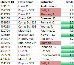
Note: You can’t conditionally format fields in the Values area of a PivotTable report by unique or duplicate values.
In the example shown here, conditional formatting is used on the Instructor column to find instructors that are teaching more than one class (duplicate instructor names are highlighted in a pale red color). Grade values that are found just once in the Grade column (unique values) are highlighted in a green color.
Quick formatting
-
Select the cells that you want to conditionally format.
-
On the Home tab, in the Style group, click the arrow next to Conditional Formatting, and then click Highlight Cells Rules.
-
Select Duplicate Values.
-
Enter the values you want to use, and then select a format.
Advanced formatting
-
Select the cells that you want to conditionally format.
-
On the Home tab, in the Styles group, click the arrow next to Conditional Formatting, and then click Manage Rules. The Conditional Formatting Rules Manager dialog box appears.
-
Do one of the following:
-
To add a conditional format, click New Rule. The New Formatting Rule dialog box appears.
-
To add a new conditional format based on one that is already listed, select the rule, then click Duplicate Rule. The duplicate rule is copied and appears in the dialog box. Select the duplicate, then select Edit Rule. The Edit Formatting Rule dialog box appears.
-
To change a conditional format, do the following:
-
-
Make sure that the appropriate worksheet or table is selected in the Show formatting rules for list box.
-
Optionally, change the range of cells by clicking Collapse Dialog in the Applies to box to temporarily hide the dialog box, by selecting the new range of cells on the worksheet, and then by selecting Expand Dialog.
-
Select the rule, and then click Edit rule. The Edit Formatting Rule dialog box appears.
-
-
-
Under Select a Rule Type, click Format only unique or duplicate values.
-
Under Edit the Rule Description, in the Format all list box, select unique or duplicate.
-
Click Format to display the Format Cells dialog box.
-
Select the number, font, border, or fill format you want to apply when the cell value meets the condition, and then click OK.
You can choose more than one format. The formats you select are shown in the Preview box.
If none of the above options is what you’re looking for, you can create your own conditional formatting rule in a few simple steps.
Notes: If there’s already a rule defined that you just want to work a bit differently, duplicate the rule and edit it.
-
Select Home > Conditional Formatting > Manage Rules, then in the Conditional Formatting Rule Manager dialog, select a listed rule and then select Duplicate Rule. The duplicate rule then appears in the list.
-
Select the duplicate rule, then select Edit Rule.
-
Select the cells that you want to format.
-
On the Home tab, click Conditional Formatting > New Rule.
-
Create your rule and specify its format options, then click OK.
If you don’t see the options that you want, you can use a formula to determine which cells to format — see the next section for steps).
If you don’t see the exact options you need when you create your own conditional formatting rule, you can use a logical formula to specify the formatting criteria. For example, you may want to compare values in a selection to a result returned by a function or evaluate data in cells outside the selected range, which can be in another worksheet in the same workbook. Your formula must return True or False (1 or 0), but you can use conditional logic to string together a set of corresponding conditional formats, such as different colors for each of a small set of text values (for example, product category names).
Note: You can enter cell references in a formula by selecting cells directly on a worksheet or other worksheets. Selecting cells on the worksheet inserts absolute cell references. If you want Excel to adjust the references for each cell in the selected range, use relative cell references. For more information, see Create or change a cell reference and Switch between relative, absolute, and mixed references.
Tip: If any cells contain a formula that returns an error, conditional formatting is not applied to those cells. To address this, use IS functions or an IFERROR function in your formula to return a value that you specify (such as 0, or «N/A») instead of an error value.
-
On the Home tab, in the Styles group, click the arrow next to Conditional Formatting, and then click Manage Rules.
The Conditional Formatting Rules Manager dialog box appears.
-
Do one of the following:
-
To add a conditional format, click New Rule. The New Formatting Rule dialog box appears.
-
To add a new conditional format based on one that is already listed, select the rule, then click Duplicate Rule. The duplicate rule is copied and appears in the dialog box. Select the duplicate, then select Edit Rule. The Edit Formatting Rule dialog box appears.
-
To change a conditional format, do the following:
-
-
Make sure that the appropriate worksheet, table, or PivotTable report is selected in the Show formatting rules for list box.
-
Optionally, change the range of cells by clicking Collapse Dialog in the Applies to box to temporarily hide the dialog box, by selecting the new range of cells on the worksheet or other worksheets, and then by clicking Expand Dialog.
-
Select the rule, and then click Edit rule. The Edit Formatting Rule dialog box appears.
-
-
-
Under Apply Rule To, to optionally change the scope for fields in the Values area of a PivotTable report, do the following:
-
To scope by selection: Click Selected cells.
-
To scope by corresponding field: Click All cells showing <Values field> values.
-
To scope by Value field: Click All cells showing <Values field> for <Row>.
-
-
Under Select a Rule Type, click Use a formula to determine which cells to format.
-
Under Edit the Rule Description, in the Format values where this formula is true list box, enter a formula.
You have to start the formula with an equal sign (=), and the formula must return a logical value of TRUE (1) or FALSE (0).
-
Click Format to display the Format Cells dialog box.
-
Select the number, font, border, or fill format you want to apply when the cell value meets the condition, and then click OK.
You can choose more than one format. The formats you select are shown in the Preview box.
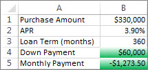
Example 1: Use two conditional formats with criteria that uses AND and OR tests
The following example shows the use of two conditional formatting rules. If the first rule doesn’t apply, the second rule applies.
First rule: a home buyer has budgeted up to $75,000 as a down payment and $1,500 per month as a mortgage payment. If both the down payment and the monthly payments fit these requirements, cells B4 and B5 are formatted green.
Second rule: if either the down payment or the monthly payment doesn’t meet the buyer’s budget, B4 and B5 are formatted red. Change some values, such as the APR, the loan term, the down payment, and the purchase amount to see what happens with the conditionally formatted cells.
Formula for first rule (applies green color)
=AND(IF($B$4<=75000,1),IF(ABS($B$5)<=1500,1))
Formula for second rule (applies red color)
=OR(IF($B$4>=75000,1),IF(ABS($B$5)>=1500,1))
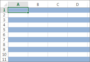
Example 2: Shade every other row by using the MOD and ROW functions
A conditional format applied to every cell in this worksheet shades every other row in the range of cells with a blue cell color. You can select all cells in a worksheet by clicking the square above row 1 and to the left of column A. The MOD function returns a remainder after a number (the first argument) is divided by divisor (the second argument). The ROW function returns the current row number. When you divide the current row number by 2, you always get either a 0 remainder for an even number or a 1 remainder for an odd number. Because 0 is FALSE and 1 is TRUE, every odd numbered row is formatted. The rule uses this formula: =MOD(ROW(),2)=1.
Note: You can enter cell references in a formula by selecting cells directly on a worksheet or other worksheets. Selecting cells on the worksheet inserts absolute cell references. If you want Excel to adjust the references for each cell in the selected range, use relative cell references. For more information, see Create or change a cell reference and Switch between relative, absolute, and mixed references.
-
The following video shows you the basics of using formulas with conditional formatting.
If you want to apply an existing formatting style to new or other data on your worksheet, you can use Format Painter to copy the conditional formatting to that data.
-
Click the cell that has the conditional formatting that you want to copy.
-
Click Home > Format Painter.
The pointer changes to a paintbrush.
Tip: You can double-click Format Painter if you want to keep using the paintbrush to paste the conditional formatting in other cells.
-
To paste the conditional formatting, drag the paintbrush across the cells or ranges of cells you want to format.
-
To stop using the paintbrush, press Esc.

Note: If you’ve used a formula in the rule that applies the conditional formatting, you might have to adjust any cell references in the formula after pasting the conditional format. For more information, see Switch between relative, absolute, and mixed references.
If your worksheet contains conditional formatting, you can quickly locate the cells so that you can copy, change, or delete the conditional formats. Use the Go To Special command to find only cells with a specific conditional format, or to find all cells that have conditional formats.
Find all cells that have a conditional format
-
Click any cell that does not have a conditional format.
-
On the Home tab, in the Editing group, click the arrow next to Find & Select, and then click Conditional Formatting.
Find only cells that have the same conditional format
-
Click any cell that has the conditional format that you want to find.
-
On the Home tab, in the Editing group, click the arrow next to Find & Select, and then click Go To Special.
-
Click Conditional formats.
-
Click Same under Data validation.
When you use conditional formatting, you set up rules that Excel uses to determine when to apply the conditional formatting. To manage these rules, you should understand the order in which these rules are evaluated, what happens when two or more rules conflict, how copying and pasting can affect rule evaluation, how to change the order in which rules are evaluated, and when to stop rule evaluation.
-
Learn about conditional formatting rule precedence
You create, edit, delete, and view all conditional formatting rules in the workbook by using the Conditional Formatting Rules Manager dialog box. (On the Home tab, click Conditional Formatting, and then click Manage Rules.)
The Conditional Formatting Rules Manager dialog box appears.
When two or more conditional formatting rules apply, these rules are evaluated in order of precedence (top to bottom) by how they are listed in this dialog box.
Here’s an example that has expiration dates for ID badges. We want to mark badges that expire within 60 days but are not yet expired with a yellow background color, and expired badges with a red background color.
In this example, cells with employee ID numbers who have certification dates due to expire within 60 days are formatted in yellow, and ID numbers of employees with an expired certification are formatted in red. The rules are shown in the following image.
The first rule (which, if True, sets cell background color to red) tests a date value in column B against the current date (obtained by using the TODAY function in a formula). Assign the formula to the first data value in column B, which is B2. The formula for this rule is =B2<TODAY(). This formula tests the cells in column B (cells B2:B15). If the formula for any cell in column B evaluates to True, its corresponding cell in column A (for example, A5 corresponds to B5, A11 corresponds to B11), is then formatted with a red background color. After all the cells specified under Applies to are evaluated with this first rule, the second rule is tested. This formula checks if values in the B column are less than 60 days from the current date (for example, suppose today’s date is 8/11/2010). The cell in B4, 10/4/2010, is less than 60 days from today, so it evaluates as True, and is formatted with a yellow background color. The formula for this rule is =B2<TODAY()+60. Any cell that was first formatted red by the highest rule in the list is left alone.
A rule higher in the list has greater precedence than a rule lower in the list. By default, new rules are always added to the top of the list and therefore have a higher precedence, so you’ll want to keep an eye on their order. You can change the order of precedence by using the Move Up and Move Down arrows in the dialog box.
-
What happens when more than one conditional formatting rule evaluates to True
Sometimes you have more than one conditional formatting rule that evaluates to True. Here’s how rules are applied, first when rules don’t conflict, and then when they do conflict:
When rules don’t conflict For example, if one rule formats a cell with a bold font and another rule formats the same cell with a red color, the cell is formatted with both a bold font and a red color. Because there is no conflict between the two formats, both rules are applied.
When rules conflict For example, one rule sets a cell font color to red and another rule sets a cell font color to green. Because the two rules are in conflict, only one can apply. The rule that is applied is the one that is higher in precedence (higher in the list in the dialog box).
-
How pasting, filling, and the Format Painter affect conditional formatting rules
While editing your worksheet, you may copy and paste cell values that have conditional formats, fill a range of cells with conditional formats, or use the Format Painter. These operations can affect conditional formatting rule precedence in the following way: a new conditional formatting rule based on the source cells is created for the destination cells.
If you copy and paste cell values that have conditional formats to a worksheet opened in another instance of Excel (another Excel.exe process running at the same time on the computer), no conditional formatting rule is created in the other instance and the format is not copied to that instance.
-
What happens when a conditional format and a manual format conflict
If a conditional formatting rule evaluates as True, it takes precedence over any existing manual format for the same selection. This means that if they conflict, the conditional formatting applies and the manual format does not. If you delete the conditional formatting rule, the manual formatting for the range of cells remains.
Manual formatting is not listed in the Conditional Formatting Rules Manager dialog box nor is it used to determine precedence.
-
Controlling when rule evaluation stops by using the Stop If True check box
For backwards compatibility with versions of Excel earlier than Excel 2007, you can select the Stop If True check box in the Manage Rules dialog box to simulate how conditional formatting might appear in those earlier versions of Excel that do not support more than three conditional formatting rules or multiple rules applied to the same range.
For example, if you have more than three conditional formatting rules for a range of cells, and are working with a version of Excel earlier than Excel 2007, that version of Excel:
-
Evaluates only the first three rules.
-
Applies the first rule in precedence that is True.
-
Ignores rules lower in precedence if they are True.
The following table summarizes each possible condition for the first three rules:
If rule
Is
And if rule
Is
And if rule
Is
Then
One
True
Two
True or False
Three
True or False
Rule one is applied and rules two and three are ignored.
One
False
Two
True
Three
True or False
Rule two is applied and rule three is ignored.
One
False
Two
False
Three
True
Rule three is applied.
One
False
Two
False
Three
False
No rules are applied.
You can select or clear the Stop If True check box to change the default behavior:
-
To evaluate only the first rule, select the Stop If True check box for the first rule.
-
To evaluate only the first and second rules, select the Stop If True check box for the second rule.
You can’t select or clear the Stop If True check box if the rule formats by using a data bar, color scale, or icon set.
-

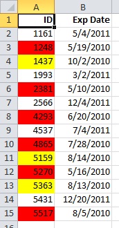
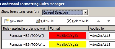
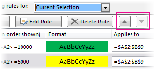
If you’d like to watch a video showing how to manage conditional formatting rules, see Video: Manage conditional formatting.
The order in which conditional formatting rules are evaluated — their precedence — also reflects their relative importance: the higher a rule is on the list of conditional formatting rules, the more important it is. This means that in cases where two conditional formatting rules conflict with each other, the rule that is higher on the list is applied and the rule that is lower on the list is not applied.
-
On the Home tab, in the Styles group, click the arrow next to Conditional Formatting, and then click Manage Rules.
The Conditional Formatting Rules Manager dialog box appears.
The conditional formatting rules for the current selection are displayed, including the rule type, the format, the range of cells the rule applies to, and the Stop If True setting.
If you don’t see the rule that you want, in the Show formatting rules for list box, make sure that the right range of cells, worksheet, table, or PivotTable report is selected.
-
Select a rule. Only one rule can be selected at a time.
-
To move the selected rule up in precedence, click Move Up. To move the selected rule down in precedence, click Move Down.
-
Optionally, to stop rule evaluation at a specific rule, select the Stop If True check box.
Clear conditional formatting on a worksheet
-
On the Home tab, click Conditional Formatting > Clear Rules > Clear Rules from Entire Sheet.
Follow these steps if you have conditional formatting in a worksheet, and you need to remove it.
For an entire
worksheet
-
On the Home tab, click Conditional Formatting > Clear Rules > Clear Rules from Entire Sheet.
In a range of cells
-
Select the cells that contain the conditional formatting.
-
Click the Quick Analysis Lens
button that appears to the bottom right of the selected data.Notes:
Quick Analysis Lens will not be visible if:-
All of the cells in the selected range are empty, or
-
There is an entry only in the upper-left cell of the selected range, with all of the other cells in the range being empty.
-
-
Click Clear Format.
 button that appears to the bottom right of the selected data.
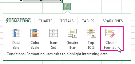
Find and remove the same conditional formats throughout a worksheet
-
Click on a cell that has the conditional format that you want to remove throughout the worksheet.
-
On the Home tab, click the arrow next to Find & Select, and then click Go To Special.
-
Click Conditional formats.
-
Click Same under Data validation. to select all of the cells that contain the same conditional formatting rules.
-
On the Home tab, click Conditional Formatting > Clear Rules > Clear Rules from Selected Cells.
Tip: The following sections use examples so you can follow along in Excel for the web. To start, download the Conditional Formatting Examples workbook and save it to OneDrive. Then, open OneDrive in a web browser and select the downloaded file.
-
Select the cells you want to format, then select Home > Styles > Conditional Formatting > New Rule. You can also open the Conditional Formatting pane and create a new rule without first selecting a range of cells.
-
Verify or adjust the cells in Apply to range.
-
Choose a Rule Type and adjust the options to meet your needs.
-
When finished, select Done and the rule will be applied to your range.
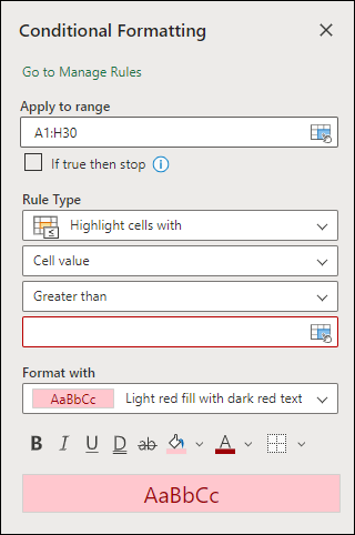
-
Select a cell which has a conditional format you want to change. Or you can select Home > Styles > Conditional Formatting > Manage Rules to open the Conditional Formatting task pane and select an existing rule.
-
The Conditional Formatting task pane displays any rules which apply to specific cells or ranges of cells.
-
Hover over the rule and select Edit by clicking the pencil icon. This opens the task pane for rule editing.
-
Modify the rule settings and click Done to apply the changes.
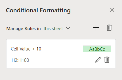
The Conditional Formatting task pane provides everything you need for creating, editing, and deleting rules. Use Manage Rules to open the task pane and work with all the Conditional Formatting rules in a selection or a sheet.
-
In an open workbook, select Home > Styles > Conditional Formatting > Manage Rules.
-
The Conditional Formatting task pane opens and displays the rules, scoped to your current selection.
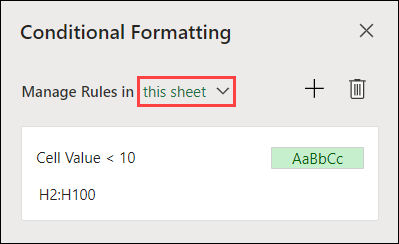
From here, you can:
-
Choose a different scope on the Manage Rules in menu — for example, choosing this sheet tells Excel to look for all rules on the current sheet.
-
Add a rule by selecting New Rule (the plus sign).
-
Delete all rules in scope by selecting Delete All Rules (the garbage can).
You can use a formula to determine how Excel evaluates and formats a cell. Open the Conditional Formatting pane and select an existing rule or create a new rule.
In the Rule Type dropdown, select Formula.
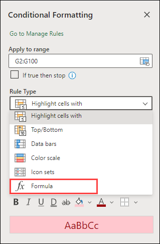
Enter the formula in the box. You can use any formula that returns a logical value of TRUE (1) or FALSE (0), but you can use AND and OR to combine a set of logical checks.
For example, =AND(B3=»Grain»,D3<500) is true for a cell in row 3 if both B3=»Grain» and D3<500 are true.
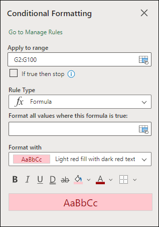
You can clear conditional formatting in selected cells or the entire worksheet.
-
To clear conditional formatting in selected cells, select the cells in the worksheet. Then Select Home > Styles > Conditional Formatting > Clear Rules > Clear Rules from Selected Cells.
-
To clear conditional formatting in the entire worksheet, select Home > Styles > Conditional Formatting > Clear Rules > Clear Rules from Entire Sheet.
-
To delete conditional formatting rules, select Home > Styles > Conditional Formatting >Manage Rules and use the delete (garbage can) on a specific rule or the Delete all rules button.
Color scales are visual guides which help you understand data distribution and variation. Excel offers both two-color scales and three-color scales.
A two-color scale helps you compare a range of cells by using a gradation of two colors. The shade of the color represents higher or lower values. For example, in a green and yellow color scale, you can specify that higher value cells be more green and lower value cells have a more yellow.
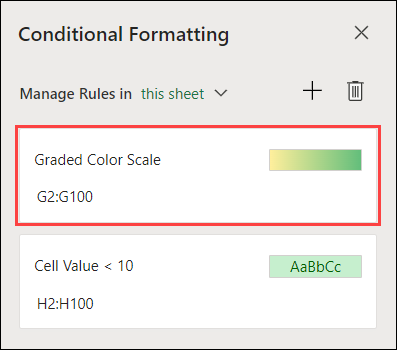
A three-color scale helps you compare a range of cells by using a gradation of three colors. The shade of the color represents higher, middle, or lower values. For example, in a green, yellow, and red color scale, you can specify that higher value cells have a green color, middle value cells have a yellow color, and lower value cells have a red color.
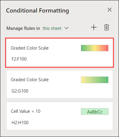
Tip: You can sort cells that have one of these formats by their color — just use the context menu.
-
Select the cells that you want to conditionally format using color scales.
-
Click Home > Styles > Conditional Formatting > Color Scales and select a color scale.
A data bar helps you see the value of a cell relative to other cells. The length of the data bar represents the value in the cell. A longer bar represents a higher value, and a shorter bar represents a lower value. Data bars are useful in spotting higher and lower numbers, especially with large amounts of data, such as top selling and bottom selling toys in a holiday sales report.
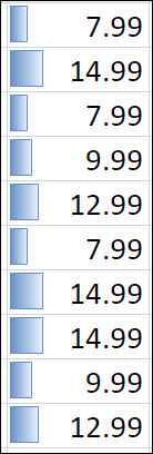
-
Select the cells that you want to conditionally format.
-
Select Home > Styles > Conditional Formatting > Data Bars and select a style.
Use an icon set to annotate and classify data into three to five categories separated by a threshold value. Each icon represents a range of values. For example, in the 3 Arrows icon set, the green up arrow represents higher values, the yellow sideways arrow represents middle values, and the red down arrow represents lower values.
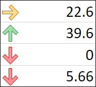
-
Select the cells that you want to conditionally format.
-
Select Home > Styles > Conditional Formatting > Icon Sets and choose an icon set.
This option lets you highlight specific cell values within a range of cells based on their specific contents. This can be especially useful when working with data sorted using a different range.
For example, in an inventory worksheet sorted by categories, you could highlight the names of products where you have fewer than 10 items in stock so it’s easy to see which products need restocking without resorting the data.
-
Select the cells that you want to conditionally format.
-
Select Home > Styles > Conditional Formatting > Highlight Cell Rules.
-
Select the comparison, such as Between, Equal To, Text That Contains, or A Date Occurring.
You can highlight the highest and lowest values in a range of cells which are based on a specified cutoff value.
Some examples of this would include highlighting the top five selling products in a regional report, the bottom 15% products in a customer survey, or the top 25 salaries in a department.
-
Select the cells that you want to conditionally format.
-
Select Home > Styles > Conditional Formatting > Top/Bottom Rules.
-
Select the command you want, such as Top 10 items or Bottom 10 %.
-
Enter the values you want to use, and select a format (fill, text, or border color).
You can highlight values above or below an average or standard deviation in a range of cells.
For example, you can find the above-average performers in an annual performance review, or locate manufactured materials that fall below two standard deviations in a quality rating.
-
Select the cells that you want to conditionally format.
-
Select Home> Styles > Conditional Formatting > Top/Bottom Rules.
-
Select the option you want, such as Above Average or Below Average.
-
Enter the values you want to use, and select a format (fill, text, or border color).
-
Select the cells that you want to conditionally format.
-
Select Home > Styles > Conditional Formatting > Highlight Cell Rules > Duplicate Values.
-
Enter the values you want to use, and select a format (fill, text, or border color).
If you want to apply an existing formatting style to other cells on your worksheet, use Format Painter to copy the conditional formatting to that data.
-
Click the cell that has the conditional formatting you want to copy.
-
Click Home > Format Painter.
The pointer will change to a paintbrush.
Tip: You can double-click Format Painter if you want to keep using the paintbrush to paste the conditional formatting in other cells.
-
Drag the paintbrush across the cells or range of cells you want formatted.
-
To stop using the paintbrush, press Esc.
Note: If you’ve used a formula in the rule that applies the conditional formatting, you might have to adjust relative and absolute references in the formula after pasting the conditional format. For more information, see Switch between relative, absolute, and mixed references.
Note: You can’t use conditional formatting on external references to another workbook.
Need more help?
You can always ask an expert in the Excel Tech Community or get support in the Answers community.
See Also
Conditional formatting compatibility issues
Skip to content
В этой статье вы найдете множество быстрых способов как сделать условное форматирование строк, столбцов и отдельных ячеек в MS Excel 2016, 2013 и 2010. Мы рассмотрим, как можно применить различное оформление к данным, которые соответствуют определенным критериям. Это может помочь указать на наиболее важную информацию в ваших электронных таблицах.
Всем известно, что изменить фон ячейки легко. Это можно совершить, просто нажав кнопку «Цвет заливки». Но что, если вы хотите изменить оформление вашей таблицы при выполнении какого-то условия? Более того, что, если вам нужно, чтобы он изменялся автоматически при внесении изменений в таблицу? Условное форматирование для этого является действительно мощной и полезной функцией. Далее в этой статье вы найдете ответы на эти вопросы и прочтете несколько полезных советов, которые помогут выбрать правильный метод условного форматирования для каждой конкретной задачи.
В то же время изменение внешнего вида в связи с содержанием текущей либо какой-то иной ячейки либо от иных условий часто считается одной из самых сложных и непонятных функций, особенно для новичков. Если вас тоже пугает эта функция, не бойтесь! На самом деле, она очень удобна и проста в использовании, и вы убедитесь в этом всего за 5 минут после прочтения этого руководства. А теперь взгляните, сколько всего мы можем сделать!
- Где находится форматирование по условию в Excel?
- Как автоматически изменить цвет при помощи условного форматирования?
- Условное форматирование Excel по значению ячейки.
- Использование абсолютных и относительных ссылок в правилах.
- Как использовать в правилах ссылку на соседние листы?
- Приоритет выполнения правил — это важно!
- Как редактировать условное форматирование?
- А если забыл, где какие правила создавал?
- Как можно скопировать условное форматирование?
- Как убрать условное форматирование?
- Почему не работает?
Кроме того, если вы будете использовать форматирование по условию, то имейте в виду, что оно имеет более высокий приоритет по сравнению с обычным оформлением вручную, которое вы можете сделать через меню Главная – Формат.
Вы можете применить условное форматирование к одной или нескольким позициям, строкам, столбцам или всей таблице на основе их содержимого или при выполнении какого-то другого условия. Это делается путем создания правил (условий), в которых вы определяете, когда и как следует изменить вид выбранных клеток таблицы.
Где находится форматирование по условию в Excel?
Это очень просто: на вкладке «Главная», а в более старых версиях — группа «Стили».

Эта функция включает в себя стандартный набор заранее определенных правил и инструментов. Но главное, у пользователя есть возможность самому придумать и настроить необходимый алгоритм закраски и выделения, используя свои формулы.
Теперь, когда вы знаете, как активировать функцию условного форматирования в Excel, давайте продолжим и посмотрим, какие у вас есть варианты форматирования и как вы можете создавать свои собственные правила.
Как автоматически изменить цвет при помощи условного форматирования?
Чтобы по-настоящему использовать возможности условного формата в Excel, вы должны научиться создавать различные типы правил.
Правила условного форматирования определяют 2 ключевых момента:
- К каким ячейкам должно применяться условное форматирование,
- Какие условия должны быть выполнены.
Я покажу вам, как применить условное форматирование в Excel 2016, потому что это, кажется, самая популярная версия в наши дни. Однако оно практически не отличается от форматирования в версиях 2007, 2013 и 2010. Поэтому у вас не возникнет проблем с выделением цветом нужной информации независимо от того, какая версия установлена на вашем компьютере.
Задача: у вас есть таблица или диапазон данных, и вы хотите изменить фон ячеек на основе их содержания. Кроме того, вы хотите, чтобы он менялся динамически, отражая изменения данных.
Решение: Предположим, у вас в таблице — данные о продажах шоколада различным покупателям. Необходимо в таблице Excel закрасить цветом клетки с количеством следующим образом: менее 100 единиц товара – красным, 100 и более – зелёным.
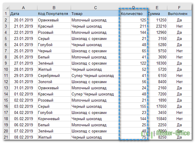
Итак, вот что вы делаете шаг за шагом:
Способ 1 — Используем стандартные возможности.
Самый простой способ — воспользоваться стандартными правилами выделения ячеек. Эти заготовки включают в себя самые простые и распространенные случаи. Но сначала выберите таблицу или диапазон, где вы хотите изменить фон ячеек. Мы взяли $D$2:$D$21.
Перейдите на вкладку «Главная» и выберите
 (1) > «Правила выделения ячеек» (2) > «Меньше» (3). В более ранних версиях программы нужное нам меню располагается в группе «Стили».
Конечно, можно использовать любой другой тип правил, который больше подходит для ваших данных, например:
- Значение больше, меньше или равно.
- Выделить текст, содержащий определённые слова или символы.
- Выделить дубликаты.
- Форматирование конкретных дат.

В диалоговом окне укажите, что числа должны быть меньше 100, также выберите вариант выделения.
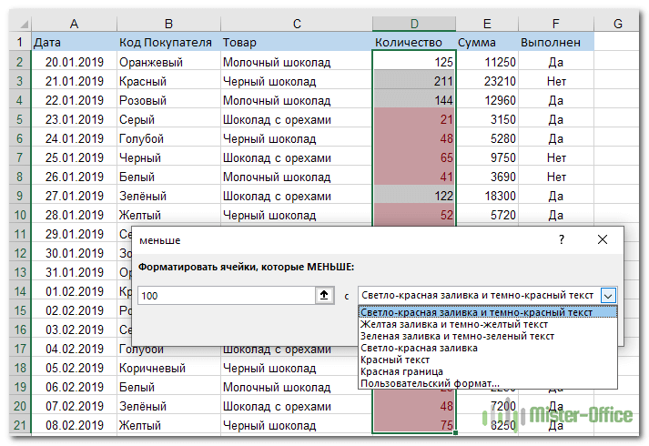
В первом поле задается условие, а во втором указывают, каким образом отформатировать полученный результат. Обратите внимание, выбрать можно цвет фона и текста из предложенных в списке. Но если хочется применить иные оттенки – сделать это можно, перейдя в «Пользовательский формат».
В результате клетки таблицы с количеством меньше 100 окрасились в красный цвет.
Приступаем к созданию второго правила. С этой же областью таблицы проделайте те же операции, только выберите на третьем шаге пункт «Больше».
В результате получим нужную нам раскраску.

Это самый простой вариант заливки ячеек.
С помощью использованных нами «Правил выделения ячеек»:
- находят в таблице числа, которые больше определенного;
- выбирают те, которые меньше определенного;
- указывают на числа, находящиеся в пределах нужного интервала;
- определяют равные какому-то числу;
- помечают в выбранных текстовых полях только те, которые необходимы;
- отмечают столбцы и числа за нужную дату;
- находят повторяющиеся текст или числа;
- придумывают прочие правила.
Способ 2 — Как самому создать правило форматирования?
Тот же результат мы можем получить и чуть иначе. Если ни одно из готовых правил форматирования не отвечает вашим потребностям, вы можете создать новое с нуля. Для этого вновь перейдите на вкладку «Главная» и выберите (1 на рисунке) > «Создать правило» (2).
Затем выберите пункт «Форматировать только ячейки, которые содержат» (3). Чуть ниже укажите, что число должно быть меньше (4) цифры «100» (5).
И далее укажите, как это все должно выглядеть. Нажмите кнопку «Формат» (6).
Выберите «красный» на открывшейся вкладке «Заливка».
Нажмите «ОК».
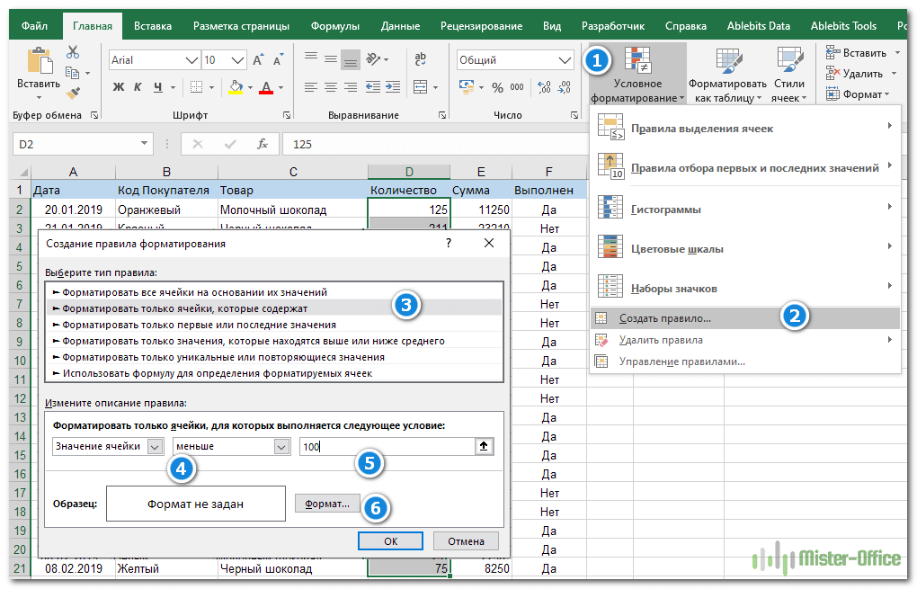
При создании правила в окне « Формат ячеек» переключайтесь между вкладками « Шрифт» , « Граница» и « Заливка», чтобы выбрать стиль шрифта, стиль рамки и цвет фона соответственно. На вкладках Шрифт и Заливка вы сразу увидите предварительный просмотр вашего пользовательского формата.
Когда закончите, нажмите кнопку ОК в нижней части окна.
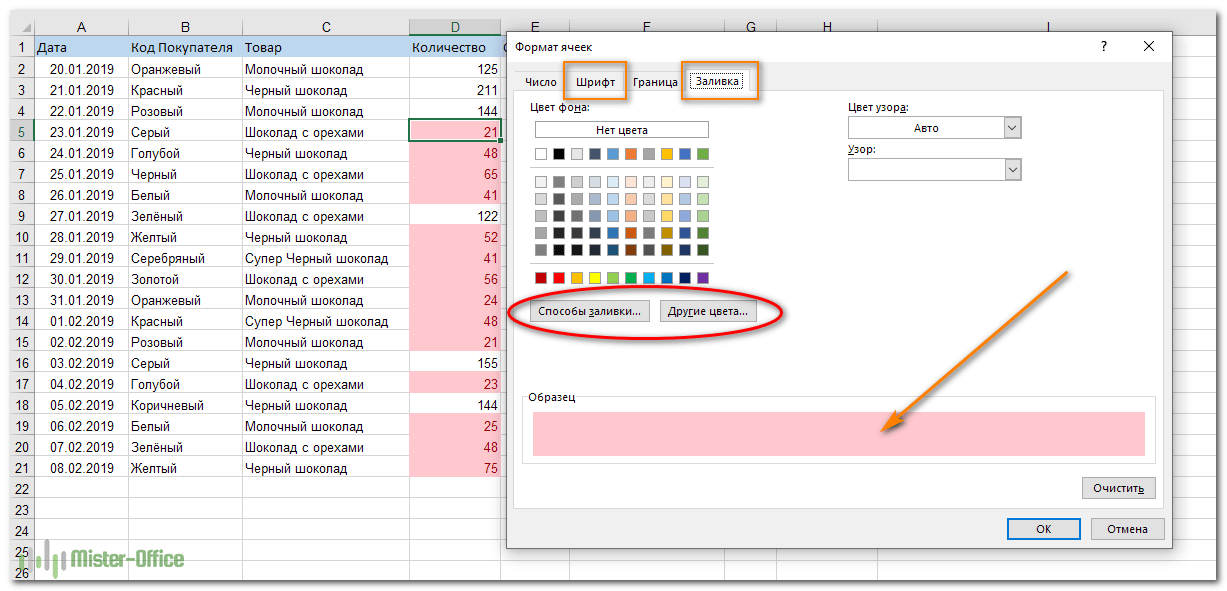
Подсказка:
Если вам нужно больше цветов фона или шрифта, чем предусмотрено в стандартной палитре, нажмите кнопку «Другие цвета…» на вкладках «Заливка» и «Шрифт»..
Если вы хотите применить градиент цвета фона , нажмите кнопку «Способы заливки» и выберите нужные параметры.
Нажмите кнопку ОК, чтобы закрыть окно и проверить, правильно ли применяется условное форматирование к вашим данным.
Повторите все то же самое еще раз, только измените условие: цифра должна быть больше или равна 100. И новый цвет условного форматирования, конечно же, выберите сейчас зеленый.
Способ 3 — Применяем собственную формулу в правиле условного форматирования.
И, наконец, третий способ – самый сложный, но зато самый универсальный и с большими возможностями. Чуть ранее мы создали правила форматирования, указав определенные числа, дату либо текст. Однако в некоторых случаях имеет смысл основывать условие на значении определенной ячейки. Преимущество этого подхода состоит в том, что в зависимости от того, как значение этой ячейки изменится в будущем, ваше условное форматирование будет корректироваться автоматически и отражать изменение данных.
Вновь перейдите на вкладку «Главная», (в старых версиях программы — в группу «Стили») и выберите (1) > «Создать правило» (2).
Затем выберите пункт «Использовать формулу для определения форматируемых ячеек» (3). Теперь нужно указать диапазон, в котором мы хотим что-то выделить. Для этого нажмите на пиктограмму со стрелкой вверх (4) и укажите мышкой начало диапазона – D2. Следите за тем, чтобы ссылка не была абсолютной (можно для этого использовать F4). И в конце просто допишите условие: “<100” (5), как это показано на рисунке.

Осталось только определить новые правила форматирования. Нажмите кнопку «Формат» (6).
Выберите красный на вкладке «Заливка».
Повторите создание условия еще раз, только выражение запишите D2>=100 и выберите зеленый.
Вы спросите: «А зачем все так сложно, если есть более простой вариант?» Дело в том, что использование формулы – более универсальный подход, который мы в дальнейшем будем еще неоднократно применять.
Итак, цель достигнута: фон выбранных ячеек изменяется от их наполнения.
Совет: вы можете использовать тот же метод не только для закраски, но и для изменения оформления шрифта. Для этого просто перейдите на вкладку «Шрифт» в диалоговом окне «Формат», которое мы обсуждали на шаге 6, и выберите предпочитаемый вариант оформления.
Условное форматирование Excel по значению ячейки.
В обоих предыдущих примерах мы создали правила форматирования, прямо указав числа — ограничения. Но чаще всего следует создавать критерий форматирования на основе значений ячеек. Как это сделать? Предположим, в таблице записаны ежемесячные продажи нескольких товаров. Нужно выделить цветом те цифры в декабре, которые были больше январских, в начале года.
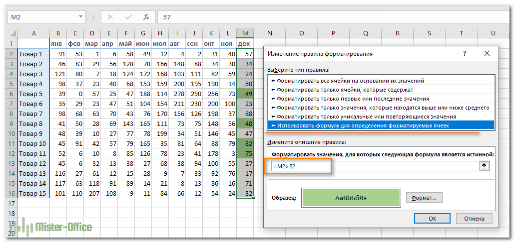
Выделяем область для применения условного форматирования М2:М16 и затем выбираем пункт «Создать правило». В описании правила запишем выражение:
=M2>B2
Обратите внимание, что здесь используются относительные ссылки, чтобы программа могла последовательно перебрать все ячейки указанной ей области, и при этом каждой ячейке из столбца М соответствовала ячейка из столбца В, расположенная в той же строке и относящаяся к тому же самому товару.
Отображение выделенных ячеек настройте так же, как мы это рассматривали ранее.
Как видно на рисунке, созданное нами правило условного форматирования работает правильно и выделяет декабрьские продажи тех товаров, которые выросли по сравнению с январём.
Использование абсолютных и относительных ссылок в правилах.
Для того, чтобы было проще изменять условия выделения определенных значений в таблице Эксель, запишем некоторые параметры отбора в специально отведённые для этого ячейки.
Задача: выделить в таблице заказы с количеством менее 50 и более 100 ед.

Наши ограничения записываем в D1 и D2. Далее создаем первое правило условного форматирования для диапазона E5:E24.
=E5>$D$2
Абсолютная ссылка на D2 означает, что каждая из ячеек нашего диапазона сравнения должна сравниваться именно с D2. А относительная ссылка на первую ячейку нашей выделенной области E5 предписывает программе начать именно с этой позиции и последовательно двигаться вниз по столбцу, сравнивая количество с пороговым значением 100.
Как обычно, выбираем цвет заливки в случае выполнения условия.
Аналогичным образом для E5:E24 создаем второе правило
=E5<$D$1
В результате часть столбца окрасится зелёным, часть — жёлтым, а количество между 50 и 100 останется неокрашенным.
А теперь давайте усложним задачу — закрасим цветом не отдельные ячейки, а строки таблицы целиком. Для этого нам всего лишь понадобится изменить несколько ссылок в наших правилах.
Прежде всего, заново обозначим диапазон условного форматирования. Теперь это будет $A$5:$G$24.
В правило форматирования внесем небольшое изменение:
=$E5>$D$2
Как видите, у нас появилась абсолютная ссылка на столбец E. А на строку ссылка осталась относительной, без знака $. Для программы это означает, что нужно использовать данные строки целиком, и окрасить ее тоже всю, а не отдельную ячейку.
Аналогично второе условие мы меняем с E5<$D$1 на $E5<$D$1.
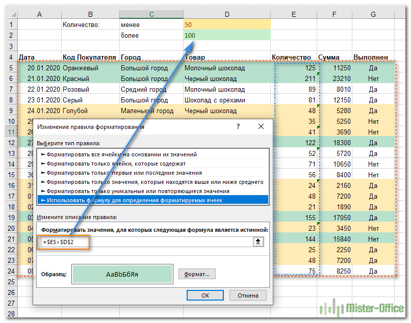
В то же время ссылка на D2 так и остается абсолютной, поскольку условие записано именно в этой ячейке. В результате получаем «полосатую» таблицу, где цветом выделены уже целые строки. И вся хитрость заключается в грамотном использовании абсолютных ссылок в правилах.
Вывод. Давайте постараемся запомнить несложные принципы использования ссылок в правилах:
- если сравниваются попарно 2 столбца, то используют относительные ссылки (M2>B2).
- если значения в столбце сопоставляются с определённой ячейкой, то на нее обязательно должна быть абсолютная ссылка ($D$1).
- когда нужно закрасить по условию строку целиком, то ссылка на эту строку должна быть относительной ($E5)
- когда нужно закрасить столбец целиком, то ссылка на него должна быть относительной (E$5)
Как использовать в правилах ссылку на соседние листы?
В последних версиях начиная с 2010 года, в формулах условия вы можете спокойно использовать ссылки на данные с других листов. Делается это точно так же, как и в обычных формулах.
В более ранних версиях программы – 2007 и 2003, это ограничение можно легко обойти, использовав именованные диапазоны. Вы просто присваиваете определенные имена диапазонам на текущем или на соседних листах, а затем используете эти имена в функциях.
В частности, вместо
=ЕСЛИ(‘Formatting (Лист2)’!$E$2:$E$21>5000;1;0)
можно работать по формуле
=ЕСЛИ(продажи>5000;1;0)
Как вы понимаете, диапазон ‘Formatting (Лист2)’!$E$2:$E$21 получил имя «продажи» и теперь к нему можно обратиться из любого места вашей рабочей книги.
Приоритет выполнения правил — это важно!
При использовании условного форматирования в Excel вы не ограничены только одним правилом на ячейку. Вы можете применять столько правил, сколько требует логика вашего проекта. В том случае, если в вашей таблице используется несколько правил, то важно, в каком порядке они выполняются.
Если выбрать меню «Управление правилами» и указать там «Текущий лист», то вы увидите список имеющихся правил.
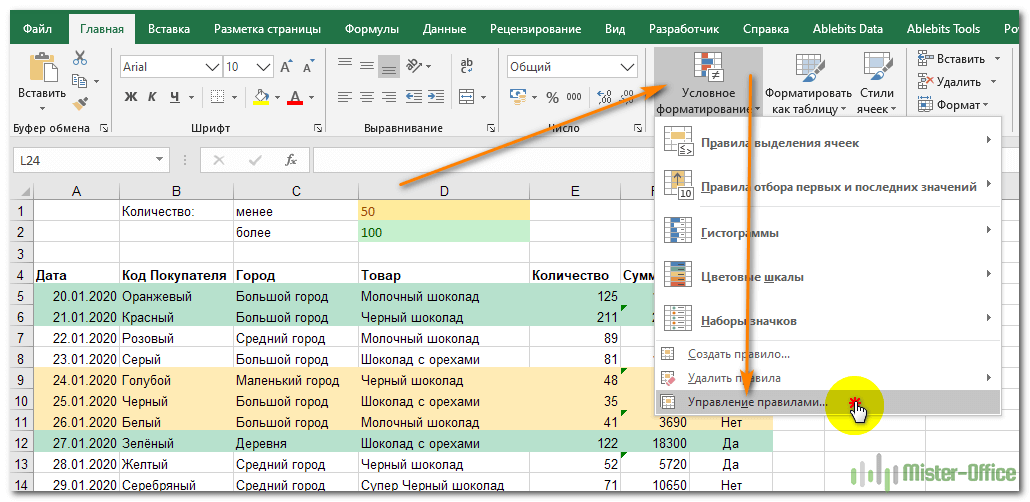
В этой таблице мы хотим выделить желтым цветом предстоящие в недалёком будущем отгрузки, а вот те из них, которые должны произойти сегодня или завтра, обозначить красным. Ведь к ним должно быть повышенное внимание и их нужно срочно выполнить.

Сначала создадим первое условие:
=$E5>$C$2
Как видим, сюда попадают все строки, в которых дата отгрузки больше текущей даты, записанной в ячейке C2.
Затем создаем второе условие, которое как бы будет являться подмножеством первого. Выделяем только ячейки, в которых ИЛИ дата отгрузки равна текущей $E$5=$C$2, ИЛИ дата отгрузки больше текущей на 1 день $E5-$C$2=1. Если хотя бы одно из этих требований выполняется, то строка будет закрашена красным.
=ИЛИ($E5-$C$2=1;$E$5=$C$2)
Важно! Правила, расположенные выше в списке, имеют более высокий приоритет (1 и 2 на рисунке вверху). Новые правила всегда добавляются в начало списка и по этой причине имеют более высокий приоритет. Результат их работы не может быть изменен действием предшествующих правил, расположенных ниже.
Однако, порядок выполнения всегда можно изменить в этом же окне при помощи стрелок «Вверх» и «Вниз» (3).
Как редактировать условное форматирование?
Для того, чтобы изменить ранее созданное условие, нужно в первую очередь посмотреть, какие условия мы применяем к таблице и далее просто выбрать нужное правило. Последовательность действий та же, что мы рассмотрели чуть выше. Но на всякий случай еще раз повторю ее на скриншоте: нам нужен раздел «Управление правилами», затем указать, что рассматриваем текущий лист.

При нажатии иконки «Изменить…» мы попадаем в уже знакомое нам меню создания правила. Только все поля там уже заполнены текущими значениями. Остается только изменить то, что необходимо, и нажать «Ок».
А если забыл, где какие правила создавал?
В виду того, что этот способ имеет приоритет над обычным оформлением, вы можете получить внешний вид таблицы не совсем таким, как ожидали. Особенно, если забудете, где и какие правила создавали. Итак, как нам быстро найти в таблице все ячейки с условным форматированием?
Один их простых способов обнаружить такие нестандартные места таблицы – использовать меню Главная – Найти и выделить – …… в последних версиях Excel. Или же Главная – Редактирование – Найти и выделить – … в более ранних версиях.
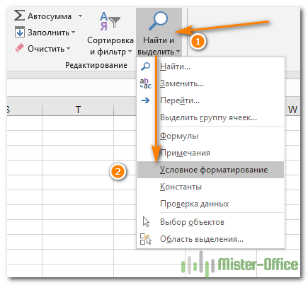
Но в результате вы просто увидите те области таблицы, в которых применено условное форматирование. И не более того. Какие именно там условия изменения оформления — пока неизвестно. В любом случае вам, скорее всего, придется копать глубже и разбираться, какие же условия там применены.
Поэтому лучше всего просто выберите раздел «Управление правилами» — текущий лист. Этот процесс мы уже дважды описывали в предыдущих разделах, поэтому, думаю, проблем здесь не возникнет.
Вы увидите все созданные вами правила, а также приоритет их выполнения. Напомним, что наивысший приоритет имеют правила, находящиеся в начале списка: чем выше, тем важнее. Также указаны области, к которым применяются созданные форматы. Думаю, здесь разобраться будет совершенно несложно.
Как можно скопировать условное форматирование?
Вот несколько способов для копирования правил.
Копировать формат по образцу
Можно скопировать так же, как и обычный формат.
На вкладке «Главная» в самом начале ленты расположена группа «Буфер обмена». В ней вы видите пиктограмму кисти – формат по образцу (в разных версия выглядит по-разному, но называется одинаково). Клик по ней копирует не только формат выделенных ячеек, но и условия для него, если таковые имеются. Следующим действием необходимо выделить те ячейки, в которые данное оформление необходимо перенести.
Имейте в виду, что описанный способ перенесет абсолютно все форматы, в том числе и установленные вручную.
Копирование через вставку.
Альтернативным вариантом дублировать формат является специальный способ вставки.
Скопируйте ячейки с нужным условным форматом любым привычным для вас способом. Выделите диапазон, на который требуется перенести формат (можете выделить и не смежные, зажав клавишу CTRL), а затем по щелчку правой кнопки мыши выберите пункт «Специальная вставка…». Тогда программа отобразит окно, где потребуется установить переключатель на точке «форматы», после чего нажать «OK».
Управление правилами.
Можно воспользоваться диспетчером правил.
Пройдите по следующему пути: -> «Управление правилами…».

Из раскрывающего списка «Показать правила…» выберите пункт «Этот лист». Вы сможете увидеть все правила, которые действуют на текущем листе.
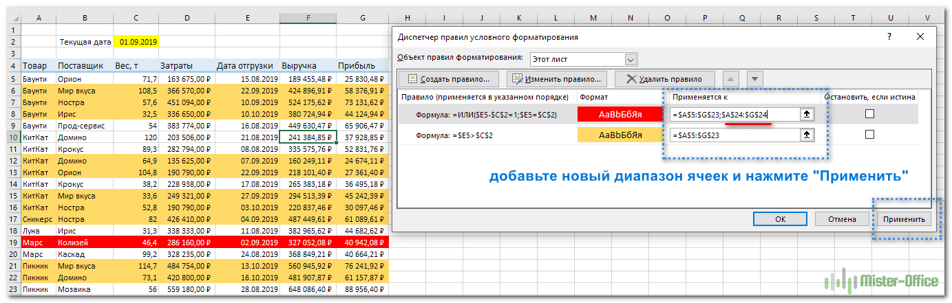
В столбце списка правил «Применяется к» указаны диапазоны, на которые распространяется каждое правило. Допишите в это поле через точку с запятой нужные адреса ячеек, чтобы применить и к ним ранее созданные условия.
Данный способ более трудоемкий, чем предыдущие два. Но его прелесть в том, что он позволяет распространять только нужные правила. Это особенно полезно тогда, когда к копируемым ячейкам применяется несколько условий одновременно, а скопировать нужно только одно из них.
Как убрать условное форматирование?
Эта операция такая же несложная, как и создание правила. Выберите , и затем – «Удалить правила». Вам будет предложено либо удаление из выделенного диапазона данных, либо вовсе всех правил на листе. Но имейте в виду, что при этом вы удалите всё, что было ранее создано. А ведь, возможно, что-то вы хотели бы сохранить.
Поэтому существует и более тонкий инструмент, которым мы рекомендовали бы пользоваться и для редактирования, и для их удаления.
Используйте последний пункт выпадающего меню: «Управление правилами».
Здесь вы видите все правила на текущем листе, к каким диапазонам они относятся и что делают. Поэтому гораздо проще выбрать определенное правило и удалить его.
Либо изменить, если в этом есть необходимость.
Почему не работает?
Если вы не получаете ожидаемого результата, то в первую очередь следует убедиться, верно ли работает созданное вами правило условного форматирования. Для этого вы можете скопировать формулу из правила в любую пустую ячейку и посмотреть, какой результат будет получен. Если вы форматируете по условию целый столбец цифр, то выберите пустое место справа от вашей таблицы.
Если результатом выполнения формулы-условия будет ИСТИНА, значит, должно быть применено условное форматирование. Естественно, если ЛОЖЬ, то — нет. Давайте вернемся в одной из наших задач и выполним такую отладку правил форматирования.

В столбец I скопируем формулу первого условия, в K — второго. Зацепите мышкой правый нижний уголок ячейки с формулой и протащите ее вниз на всю высоту таблицы. Получим полную картину для каждой из ячеек нашего диапазона. Как видите, ИСТИНА и ЛОЖЬ точно соответствуют закраске столбца K, который мы, собственно, и проверяли. В I2 мы получили ИСТИНА, поэтому цвет — зелёный. В J9 ответ также положительный, поэтому цвет — желтый. И так далее.
Если формула сложная, можно разбить ее на части и применить тот же метод отладки.
Надеемся, что вы нашли ответы на интересующие вас вопросы по условному форматированию в нашей инструкции.
Тем не менее, если всё же что-то не получается или не работает – пишите в комментариях ниже. Мы постараемся вам ответить либо даже сделаем отдельный материал, посвященный вашей проблеме.
Удачи!
Еще полезные примеры и советы:
 Формат времени в Excel — Вы узнаете об особенностях формата времени Excel, как записать его в часах, минутах или секундах, как перевести в число или текст, а также о том, как добавить время с помощью…
  Как сделать пользовательский числовой формат в Excel — В этом руководстве объясняются основы форматирования чисел в Excel и предоставляется подробное руководство по созданию настраиваемого пользователем формата. Вы узнаете, как отображать нужное количество десятичных знаков, изменять выравнивание или цвет шрифта,…
  7 способов поменять формат ячеек в Excel — Мы рассмотрим, какие форматы данных используются в Excel. Кроме того, расскажем, как можно быстро изменять внешний вид ячеек самыми различными способами. Когда дело доходит до форматирования ячеек в Excel, большинство…
  9 способов сравнить две таблицы в Excel и найти разницу — В этом руководстве вы познакомитесь с различными методами сравнения таблиц Excel и определения различий между ними. Узнайте, как просматривать две таблицы рядом, как использовать формулы для создания отчета о различиях, выделить…
На чтение 2 мин
Функция AND (И) в Excel используется для сравнения нескольких условий.
Содержание
- Что возвращает функция
- Синтаксис
- Аргументы функции
- Дополнительная информация
- Примеры использования функции AND (И, ИЛИ) в Excel
Что возвращает функция
Возвращает TRUE если значение или условие, при сравнении, соответствует критериям заданным в функции, или FALSE, в случае, если условие не соответствует критериям.
Синтаксис
=AND(logical1, [logical2],…) — английская версия
=И(логическое_значение1;[логическое_значение2];…) — русская версия
Аргументы функции
- logical1 (логическое_значение1) — первое условие, которое вы хотите оценить с помощью функции;
- [logical2] ([логическое_значение2]) (не обязательно) — второе условие, которое вы хотите оценить с помощью функции.
Дополнительная информация
- Функция может быть использована совместно с другими формулами;
- Например, с помощью функции IF (ЕСЛИ) вы можете проверить условие, а затем указать значение, когда оно TRUE, и значение, когда оно равно FALSE. Использование функции AND (И) вместе с функцией IF (ЕСЛИ) позволяет тестировать несколько условий за один раз;
Например, если вы хотите проверить значение в ячейке A1 на предмет того, больше оно чем «0» или меньше чем «100», то вы можете использовать следующую формулу:
=IF(AND(A1>0,A1<100),”Approve”,”Reject”) — английская версия
=ЕСЛИ(И(A1>0;A1<100);»Одобрить»;»Против») — русская версия
- Аргументы функции должны быть логически вычислимы по принципу (TRUE/FALSE);
- Ячейки с пустыми или текстовыми значениями игнорируются функцией;
- Если в качестве аргументов функции не указаны логически вычислимые данные, то функция выдаст ошибку #VALUE!;
- Одновременно вы можете тестировать до 255 условий в рамках одного использования функции.
Примеры использования функции AND (И, ИЛИ) в Excel

Conditional formatting is a data visualization tool in several spreadsheet applications. We use it to highlight, emphasize, and differentiate by using colors or other means (like applying icons) to cells or ranges relevant to us.
At first, you will learn the essential skills. The second part of the tutorial will be about using Excel conditional formatting formulas and examples.
Table of contents:
- What is Conditional Formatting
- Learn the fundamentals of Conditional Formatting
- Highlight cells
- Highlight cells that contain text
- Edit a conditional formatting rule
- Delete a conditional formatting rule
- Conditional Formatting Formulas: Examples
Conditional formatting offers a wide range of possibilities for Excel users. Its first and foremost function is to direct attention to the most crucial data points. Then, we can determine with rules what are the most important for us. These data points can be deadlines, excellent sales results, or tasks carrying a high risk.
Download the practice file!
Fundamentals of Conditional Formatting
Before we walk you through all possibilities of conditional formatting, we have to stall a bit. It is necessary to know all the basics! First, you have to understand the structure that conditional formatting provides. So, let’s see a little overview. In short, we will summarize the most important rules for you.
Logical Operators (if-then rules): Every single conditional formatting rule is based on straightforward logic. If “X” criteria are true, then apply the rule “Y”. Let’s see a simple example: “X” criteria are: “The sales price is more than $50.” “Y” criteria are defined as a color all applicable cells red. What will happen now? By applying the if-then rule, every cell will be colored red where the sales price is > $50, more than $50.
Predefined Conditions (built-in presets): This option can interest beginners. In Excel, there are many built-in rules and conditions available. We have also thought about users with different capabilities when making the tutorial. We will learn about this subject from a detailed guide.
User-defined Conditions: There are often situations when the default settings are unsuitable for the given task. No problem, let’s make our own rules. Use the Excel formulas so we can reach the required results. We have to note that we can use all of the formulas in Excel to create the rules.
Multiple Conditions: We can simultaneously apply multiple rules for one cell or range. If there are more rules active simultaneously, which one will prevail? We will discuss this in detail in the chapter “rule hierarchy and precedence.”
Highlight Cells using rules (if the quantity is greater than 200)
Click the Highlight Cells Rules functions to highlight patterns and trends with conditional formatting. It will be straightforward to identify the cells that meet your criteria. This is a basic color formatting method for cells and ranges.
Select the range you want to use a rule and apply highlight rules. In our example, we will highlight any product that’s quantity is greater than 200 units. For example, select the range’ H2: H24′.
In the Home tab of the ribbon, click Conditional Formatting, then click Highlight Cell Rules. Finally, select ‘Greater than’.
Now, a dialog box will appear. Enter 200 In the left box. So, if you enter 200, something will happen when the value is greater than 200. But what will happen? You will define the trigger in the right box.
Explanation: Triggers can be defined in the range with which the event is associated. Just forget the standard option and select a light red fill from the drop-down list. If you click OK now, all the cells that are above 200 will be formatted based on the given rule.
Highlight cells that contain text
If you are looking for all the M types of converters in column G, you do not have to scan the screen for hours and hours. Instead, you can let conditional formatting do all the dirty work and highlight the criteria easily and automatically.
Select the range with text. In this example, you will select the range G2:G24, all our ‘Product Name.’
Click Conditional Formatting, hover the mouse over Highlight Cells Rules, and choose Text that Contains.
Enter “M type” in the text box. Next, select yellow fill color with dark yellow text using the drop-down menu, then click OK.
Tip: You can apply a custom format if the default style is unsuitable. Use the drop-down menu and select the Custom format option to create your format. You can create custom styles by changing the font, border, or fill types. Keep in mind the basics of conditional formatting! Further options are available if you can apply different rules. You can also use important highlight rules for your values: Greater than…, Equal to…, or Between.
Editing a conditional formatting rule
This section will show you how to manage conditional formatting rules. You can modify the selected rule using the conditional formatting rules manager. Use this function if you want to edit some of these rules later or delete them.
This function can be accessed using the Home Tab and the Conditional Formatting button. Then select Manage Rules from the drop-down list. By default, you’ll see a dialog box:
By default, the “Show formatting rules for:” is set to “Current Selection”. Next, select the “This Worksheet” option from the drop-down list to display the conditional formatting rules you have applied to the actual Worksheet.
Use top-bottom rules and select the rule from the list you want to modify. Then, click the rule you want to change to edit a rule. In this example, we want to highlight the top 10 values in the Total value column. Currently, the top five are highlighted.
Click the Top 5 rows! Excel highlights the selected rows with blue. Then, click Edit Rule. A dialog box opens where you can change the given conditions of the rule; type 10 in the number field. Finally, click OK.
We’ll get the Manage Rules box back. Click OK to save the changes.
Delete a conditional formatting rule
Sometimes your spreadsheet looks like a traffic jam regarding too many conditional formatting rules. This is because Excel has a hidden “feature.” If you have many unique rules, that may be the reason for the slow calculations. In this case, you should eliminate some rules in the sheet.
Tip: Excel provides a quick way to delete rules. Click the Conditional Formatting button on the Home tab and select clear rules.
But it’s not smart to delete all rules from a worksheet!
In this case, we would like to delete the rules from Column G (Product Names). Select the ‘G2:G24’ range.
To properly delete a rule, select the ‘Manage Rules’ box and click on the conditional formatting rule you want to remove.
Click OK to delete the rule.
We hope you have found the first part of the tutorial interesting and exciting. In this, we have introduced how we can use the basic rules with Excel.
Conditional Formatting and Formulas
You’ll find here 50+ formula examples and learn more about custom formulas.
All examples are based on a few simple steps:
- Select the range that you want to apply the format
- Add ‘New Rule’
- Enter the formula
- Select format style
- Click ‘OK, then click ‘Apply.’
That’s all.
Check our definitive guide with examples if you want to learn about Excel Formulas.
How do I highlight the lowest 3 values in Excel?
Create a formula to determine the 3 smallest values that meet specific criteria. Use a formula based on the AND and SMALL functions. In the example, the formula used for conditional formatting is:
=AND($B4=$E$4,$C4<=SMALL(IF(city=$E$4,sales),3))where “city” is the named range B4:B12, and “sales” is the named range C4:C12.
How to conditional format if the cell is blank?
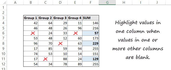
In the following example, you want to highlight values in one column when values in one or more columns are blank. A basic formula based on the OR and ISBLANK functions is used to test for blank or empty cells. For example, if any cell in a corresponding row in the range B4:E12 is blank, OR function returns TRUE. Thus, the trigger will be fired, and the cell in column F will highlight using light blue.
Use the conditional formatting formula:
=OR(ISBLANK(B4),ISBLANK(C4),ISBLANK(D4),ISBLANK(E4))How to use Conditional Formatting to highlight past due dates in Excel
You will apply a formula in the example to determine “past due dates.” The formula will check if the variance between dates is greater than a certain number of days. To create a color-coded table, use three conditional formatting rules for each interval.
Select the cells in range E4:E9 and apply the formulas.
- =(E4-D4)<5 if the variance is less than 5 days,
- =(E4-D4)<15 if the variance is between 5 days and 15 days
- =(E4-D4)>=20 if the difference between the two dates is greater than or equal to 20
Important: You have to use the stop-if-true checkbox for rule1 and rule2.
How to highlight overlapping dates in Excel
Sometimes you need to highlight cells where dates overlap. You can use conditional formatting formulas and apply the SUMPRODUCT function in the example. What are overlapping dates? We are talking about overlapping dates if these two conditions are true:
- First, the start date is less than equal to the other end dates in the column.
- The end date is greater than or equal to at least one other start date.
Create a new column to check the conditions. Then, apply the formula to cell F4 them copy the formula down.
=SUMPRODUCT(($D4<=$E$4:$E$8)*($E4>=$D$4:$D$8))>1Result:
Now create a conditional formatting rule. First, select the cells you want to format, in this case, range C4:F8. Then use the rule below to highlight overlapping dates.
=$F4=TRUE
So, click OK to apply the rule. If the result is TRUE, the given row cells in the selection will be highlighted.
Final thought
Finally, take a closer look at the advanced conditional formatting rules:
- You should know how the conditional formatting rule hierarchy works if you work with multiple rules.
- The Stop if True tool helps you to manage overlaps between rules.
- Color ranking helps you identify the maximum value in a range and highlight them.
- Learn how to use Multiple Conditions and Formulas.
Conditional formatting makes our lives in Excel a lot easier.
Use formulas wisely! We can highlight all the key information that fits the criteria. Knowing and applying conditional formatting rules decrease the time spent on data analysis. Therefore, we can be a lot more productive. We can effectively support company decisions by recognizing the patterns (whether positive or negative). Look at the in-depth article called ‘How to create an Excel Dashboard‘ regarding conditional formatting on our blog.
Additional resources
- How to use the Quick Analysis Tool
- Highlight every other row
- Compare two columns in Excel
- Build a Heat Map
- Change shape color based on cell value
- How to use data bars
- Apply colorful icon sets
- Color Scales
- Find duplicates
- How to use Conditional Formatting based on another cell
- Show protected cells