And or not syntax excel - Word и Excel - помощь в работе с программами

The IF function allows you to make a logical comparison between a value and what you expect by testing for a condition and returning a result if that condition is True or False.

=IF(Something is True, then do something, otherwise do something else)

But what if you need to test multiple conditions, where let’s say all conditions need to be True or False (AND), or only one condition needs to be True or False (OR), or if you want to check if a condition does NOT meet your criteria? All 3 functions can be used on their own, but it’s much more common to see them paired with IF functions.

Use the IF function along with AND, OR and NOT to perform multiple evaluations if conditions are True or False.

Syntax

IF(AND()) — IF(AND(logical1, [logical2], …), value_if_true, [value_if_false]))
IF(OR()) — IF(OR(logical1, [logical2], …), value_if_true, [value_if_false]))
IF(NOT()) — IF(NOT(logical1), value_if_true, [value_if_false]))


Argument name	Description
logical_test (required)	The condition you want to test.
value_if_true (required)	The value that you want returned if the result of logical_test is TRUE.

value_if_false (optional)	The value that you want returned if the result of logical_test is FALSE.

Here are overviews of how to structure AND, OR and NOT functions individually. When you combine each one of them with an IF statement, they read like this:

AND – =IF(AND(Something is True, Something else is True), Value if True, Value if False)
OR – =IF(OR(Something is True, Something else is True), Value if True, Value if False)
NOT – =IF(NOT(Something is True), Value if True, Value if False)

Examples

Following are examples of some common nested IF(AND()), IF(OR()) and IF(NOT()) statements. The AND and OR functions can support up to 255 individual conditions, but it’s not good practice to use more than a few because complex, nested formulas can get very difficult to build, test and maintain. The NOT function only takes one condition.

Here are the formulas spelled out according to their logic:

Formula	Description
=IF(AND(A2>0,B2<100),TRUE, FALSE)	IF A2 (25) is greater than 0, AND B2 (75) is less than 100, then return TRUE, otherwise return FALSE. In this case both conditions are true, so TRUE is returned.
=IF(AND(A3=»Red»,B3=»Green»),TRUE,FALSE)	If A3 (“Blue”) = “Red”, AND B3 (“Green”) equals “Green” then return TRUE, otherwise return FALSE. In this case only the first condition is true, so FALSE is returned.
=IF(OR(A4>0,B4<50),TRUE, FALSE)	IF A4 (25) is greater than 0, OR B4 (75) is less than 50, then return TRUE, otherwise return FALSE. In this case, only the first condition is TRUE, but since OR only requires one argument to be true the formula returns TRUE.
=IF(OR(A5=»Red»,B5=»Green»),TRUE,FALSE)	IF A5 (“Blue”) equals “Red”, OR B5 (“Green”) equals “Green” then return TRUE, otherwise return FALSE. In this case, the second argument is True, so the formula returns TRUE.
=IF(NOT(A6>50),TRUE,FALSE)	IF A6 (25) is NOT greater than 50, then return TRUE, otherwise return FALSE. In this case 25 is not greater than 50, so the formula returns TRUE.
=IF(NOT(A7=»Red»),TRUE,FALSE)	IF A7 (“Blue”) is NOT equal to “Red”, then return TRUE, otherwise return FALSE.

Note that all of the examples have a closing parenthesis after their respective conditions are entered. The remaining True/False arguments are then left as part of the outer IF statement. You can also substitute Text or Numeric values for the TRUE/FALSE values to be returned in the examples.

Here are some examples of using AND, OR and NOT to evaluate dates.

Here are the formulas spelled out according to their logic:

Formula	Description
=IF(A2>B2,TRUE,FALSE)	IF A2 is greater than B2, return TRUE, otherwise return FALSE. 03/12/14 is greater than 01/01/14, so the formula returns TRUE.
=IF(AND(A3>B2,A3<C2),TRUE,FALSE)	IF A3 is greater than B2 AND A3 is less than C2, return TRUE, otherwise return FALSE. In this case both arguments are true, so the formula returns TRUE.
=IF(OR(A4>B2,A4<B2+60),TRUE,FALSE)	IF A4 is greater than B2 OR A4 is less than B2 + 60, return TRUE, otherwise return FALSE. In this case the first argument is true, but the second is false. Since OR only needs one of the arguments to be true, the formula returns TRUE. If you use the Evaluate Formula Wizard from the Formula tab you’ll see how Excel evaluates the formula.
=IF(NOT(A5>B2),TRUE,FALSE)	IF A5 is not greater than B2, then return TRUE, otherwise return FALSE. In this case, A5 is greater than B2, so the formula returns FALSE.

Using AND, OR and NOT with Conditional Formatting

You can also use AND, OR and NOT to set Conditional Formatting criteria with the formula option. When you do this you can omit the IF function and use AND, OR and NOT on their own.

From the Home tab, click Conditional Formatting > New Rule. Next, select the “Use a formula to determine which cells to format” option, enter your formula and apply the format of your choice.

Using the earlier Dates example, here is what the formulas would be.

Formula	Description
=A2>B2	If A2 is greater than B2, format the cell, otherwise do nothing.
=AND(A3>B2,A3<C2)	If A3 is greater than B2 AND A3 is less than C2, format the cell, otherwise do nothing.
=OR(A4>B2,A4<B2+60)	If A4 is greater than B2 OR A4 is less than B2 plus 60 (days), then format the cell, otherwise do nothing.
=NOT(A5>B2)	If A5 is NOT greater than B2, format the cell, otherwise do nothing. In this case A5 is greater than B2, so the result will return FALSE. If you were to change the formula to =NOT(B2>A5) it would return TRUE and the cell would be formatted.

Note: A common error is to enter your formula into Conditional Formatting without the equals sign (=). If you do this you’ll see that the Conditional Formatting dialog will add the equals sign and quotes to the formula — =»OR(A4>B2,A4<B2+60)», so you’ll need to remove the quotes before the formula will respond properly.

Need more help?

What are Logical Function in Excel?

Microsoft Excel has four logical functions which can work with logical values. These functions are utilized to handle more than one comparison of values, or formulas that require one or more conditions. As well as logical operators, Excel logical functions return either TRUE or FALSE when their arguments are evaluated.

These are AND, OR, XOR, and NOT. So there is the following summary of these logical functions to help you choose the right formula for a specific task.

Function	Description	Formula Example	Formula Description
AND	This will returns TRUE if all of the arguments evaluate as TRUE.	`=AND(F2<=75, B2<70)`	The formula returns TRUE if a value in cell F2 is less than or equal to 75, and a value in B2 is less than 70, FALSE otherwise.
OR	If any argument is TRUE it will return TRUE.	`=OR(F2>=75, C2<75)`	The formula will return TRUE if A2 is greater than or equal to 75 or C2 is less than 75, or both conditions are met. If neither of the conditions is met, the formula returns FALSE.
XOR	If all arguments are exclusively logical OR.	`=XOR(F2>=75, D2<75)`	The formula returns TRUE if either F2 is greater than or equal to 75 or D2 is less than 75. If none of the conditions is met or both conditions are met, the formula returns FALSE.
NOT	This will return the reversed logical value of its argument.	`=NOT(F2>=75)`	The formula returns FALSE if a value in F2 is greater than or equal to 75; and vice versa.

The AND function of Excel comes in very handy which makes it most popular among the logical functions family. It’s used to test and meets several conditions to ensure all of them are met.

So, the AND function is for testing the specified conditions and if the evaluated condition is all TRUE then it will return TRUE otherwise it will return FALSE.

The syntax of this function is shown below:

=AND(logical1, [logical2], …)

The first argument of this syntax is required while the succeeding logical conditions are optional. Technically the logical condition to test can be evaluated as either TRUE or FALSE.

And now, let’s examine the formula examples that indicate how to use the AND functions in Excel formulas.

Formula	Description
`=AND(A2="Andrie", B2>D2)`	Returns TRUE if A2 contains “Andrie” and B2 is greater than D2, otherwise FALSE.
`=AND(F2>80, F2<E2)`	Returns TRUE if F2 is greater than 80 and F2 is less than E2, otherwise FALSE.
`=AND(A2="Andrew", F2<=75, C2>B2)`	Returns TRUE if A2 contains “Andrew”, F2 is less than or equal to 75 and C2 is greater than B2, otherwise FALSE.

And now we will use this formula and the following steps you can consider as follows.

Step 1: Prepare your numeric data in your worksheet which we will use AND function and see how it works.

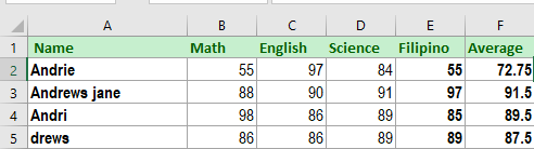
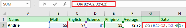
Step 2: Enter this formula in a cell you select and with two conditions here.

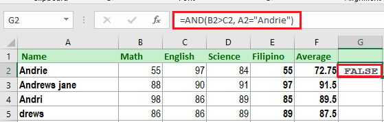
=AND(B2>C2, A2="Andrie")

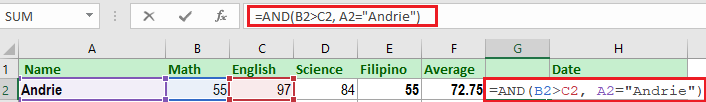
Step 3: Hit Enter to see what result we will get with the condition we input.

Hence, if it returns FALSE the first condition does not meet the first condition which B2 is greater than to C2 value. Where in we mention already AND function requires all conditions to be TRUE.

Step 4: And now, let us use again the AND function and apply it to another row of data. Below is the formula you will try with its single argument.

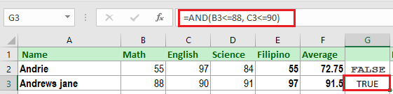
=AND(B3<=88, C3<=90)

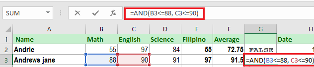
Step 5: Hit the Enter key again and you will see the result, it returns TRUE as both conditions are evaluated as TRUE.

OR function in Excel

The Excel OR function is a basic logical function that is used to evaluate statements or values. The only difference of this to AND function is if at least one statement is True it will return TRUE otherwise it will return FALSE or if all the arguments are FALSE.
Additionally, this function is available in the 2016 – 200 Excel version.

The syntax of this function is as follows:

=OR(logical1, [logical2], …)

In the same manner, the logical arguments’ test could either be TRUE or FALSE. Wherein the first argument is required and the subsequent are optional, which can up to 255 conditions in modern excel versions.

And now, let’s write down a few formulas for you to get a feel for how the OR function in Excel works.

Formula	Description
`=OR(A2="Jane", A2="Andrew")`	Returns TRUE if A2 contains “Jane” or “Andrew”, otherwise returns FALSE.
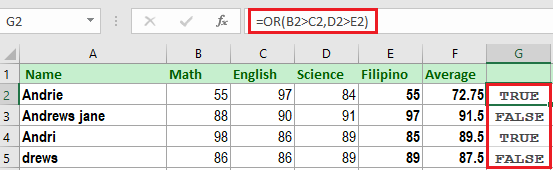
`=OR(B2>=55, C2<=97)`	Returns TRUE if B2 is greater than or equal to 55 or C2 is less than or equal to 97, otherwise return FALSE.
`=OR(F2=" ", A2="")`	Returns TRUE if either F2 or A2 is empty or both, FALSE otherwise.

Excel XOR function

Microsoft 2013 introduced this function XOR which is the exclusive OR function. So if you have any knowledge of programming languages you may encounter and familiar with this function. Meanwhile for those who are not and do not have any prior engagement with this function, the explanation below will give you an idea of how this function works.

The XOR syntax is given below:

=XOR(logical1, [logical2],…)

Where the first logical1 argument is required, the rest argument is optional. Luckily you can have up to 254 conditions you can test in just a single formula.

In simple understanding XOR function consists of two logical statements that return the following:

FALSE if all arguments are TRUE or neither is TRUE.
TRUE if at least one argument evaluates to TRUE.

This might be simple to understand from the formula examples:

Formula	Result	Description
`=XOR(10<0, 5>2)`	TRUE	Returns TRUE because the 1st argument is TRUE and the 2^nd argument is FALSE.
`=XOR(1>0, 3<5)`	FALSE	All the arguments are FALSE therefore it returns FALSE.
`=XOR(10>20, 20<1)`	FALSE	Returns FALSE because both arguments are TRUE.

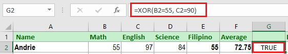
Now we will try this formula in our worksheet to test the logical test.

See the formula in the image below:

Supposedly we will have the result of TRUE.

NOT function in Excel

This NOT function in Excel is one of the simplest function, as well as its syntax.

=NOT(logical)

The arguments of this function reverse the value. In simple words, if the logical evaluates to TRUE the Not function will reverse it and return to FALSE, and vice versa.

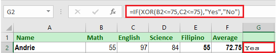
Below is the example of XOR formula which works as we want:

Here we do the nest in XOR function into the logical IF function:

Conclusion

In conclusion, logical functions in excel are helpful in worksheets especially when a formula required conditions that should be evaluated as TRUE or FALSE.

What do you think about this, feel free to leave your insights below, if you want to learn more about excel functions visit other tutorials like this.

Thank you for reading!

Источник

Excel Function AND, OR, NOT

Microsoft Excel “AND, OR, NOT Functions” are the logical functions and helps to validate the statement if said is “TRUE” or “FALSE”. “AND, OR, NOT” are the three unique logical function and each one of them has their own characteristics.

“AND, OR, NOT Functions” provide result in “TRUE” or “FALSE”. If the logical condition is correct and matching the parameters provided, then result would be “TRUE” or if logical condition is not correct and not matching the parameters provided then result would be “FALSE”

“AND, OR, NOT Functions” has only one argument i.e. (logical) and multiple logical conditions can be placed in one function. It is easy to apply for validation and output is also very to understand i.e. “TRUE” and “FALSE”. We can place multiple logical conditions in one logical statement.

Excel Function AND:

Output result of “AND” function will be “TRUE” if ALL the logical conditions of a logical statement are correct or matching as per parameters otherwise output result will be “FALSE”.

Excel Function OR:

Output result of “OR” function will be “TRUE” if ANY of the logical condition from a complete logical statement is correct or matching as per parameters otherwise output result will be “FALSE”.

“NOT” FUNCTION:

Output result of “NOT” function will be “TRUE” if NO logical conditions from a logical statement is correct or matching as per parameters otherwise output result will be “FALSE”.

Advantage of “AND, OR, NOT Functions”

“AND, OR, NOT Functions” can be used in various databases whether it is Numeric/Alpha (Strings) etc. which makes the function useful and advantageous. Applying the logical function manually (one by one) to validate if logical condition is “TRUE or FALSE” is very difficult and “AND, OR, NOT Functions” helps to apply the function in large database at once and makes the work easy, saves time and increases efficiency.

Where “AND, OR, NOT Functions” can be used:

“AND, OR, NOT Functions” are very useful and can be used in many situations. Like it can be used as follows:
– Preparing Marks summary and providing Grades as per the marks obtained
– Selection of choices from the available multiple options
– Or any other database where there is requirement placing logical conditions then “AND, OR, NOT Functions” can be used

Things to Remember:

“NOT” function can have only one logical condition, whereas “AND, OR” may have multiple logical conditions in one logical statement.
Also, we need to understand the function output. i.e. “TRUE” means logical statement is matching however “FALSE” means logical conditions are not matching. Also ensure that correct cell reference is given otherwise function output and decisions may go wrong.

“AND” Syntax:

=AND(logical1, [logical2], …)

Syntax Description:

logical, argument is used to give the logical condition. We can place multiple logical conditions to check if conditions are TRUE or FALSE.

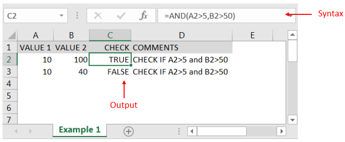
Example 1: Explore “AND” Function

“AND” function’s output will be “TRUE” only incase ALL the conditions are met. As per below example, logical statement is checking for rows# which is greater than 5 and greater than 50. Row#2 meets complete criteria that is why result is “TRUE” whereas Row#3 did not meet the second criteria (i.e. 40 is not greater than 50) that is why output result is “FALSE”

“OR” Syntax:

=OR(logical1, [logical2], ...)

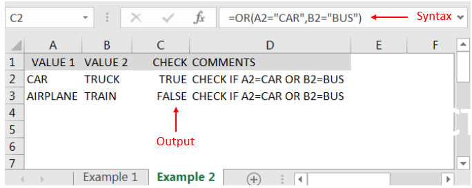
Example 2: Explore “OR” Function

“OR” function’s output will be “TRUE” in case ANY of the following condition is met. As per below example, logical statement is checking for rows# which has either CAR or BUS. Row#2 meets the one criterion out of two that is why result is “TRUE” whereas Row#3 did not meet any of the criteria (i.e. value did not have either CAR or BUS) that is why output result is “FALSE”

“NOT” Syntax:

=NOT(logical1)

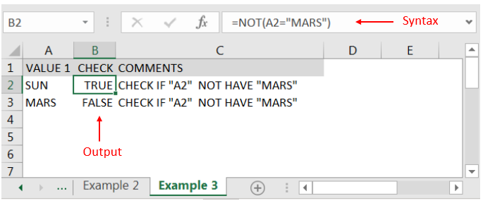
Example 3: Explore “NOT” Function

“NOT” function’s output will be “TRUE” in case NO logical conditions in a logical statement is met. As per below example, logical statement is checking for cells# which does not have “MARS”. Cell “A2” meets the criteria (i.e. Cell “A2” is SUN and not MARS”) that is why result is “TRUE” whereas output result of “A3” is “FALSE” (i.e. cell “A3” has “MARS”)

Hope you liked. Happy Learning.

Don’t forget to leave your valuable comments!

What is a Logical Function?

It is a feature that allows us to introduce decision-making when executing formulas and functions. Functions are used to;

Check if a condition is true or false
Combine multiple conditions together

What is a condition and why does it matter?

A condition is an expression that either evaluates to true or false. The expression could be a function that determines if the value entered in a cell is of numeric or text data type, if a value is greater than, equal to or less than a specified value, etc.

IF Function example

We will work with the home supplies budget from this tutorial. We will use the IF function to determine if an item is expensive or not. We will assume that items with a value greater than 6,000 are expensive. Those that are less than 6,000 are less expensive. The following image shows us the dataset that we will work with.

Put the cursor focus in cell F4
Enter the following formula that uses the IF function

=IF(E4<6000,”Yes”,”No”)

HERE,

“=IF(…)” calls the IF functions
“E4<6000” is the condition that the IF function evaluates. It checks the value of cell address E4 (subtotal) is less than 6,000
“Yes” this is the value that the function will display if the value of E4 is less than 6,000
“No” this is the value that the function will display if the value of E4 is greater than 6,000

When you are done press the enter key

You will get the following results

Excel Logic functions explained

The following table shows all of the logical functions in Excel

S/N	FUNCTION	CATEGORY	DESCRIPTION	USAGE
01	AND	Logical	Checks multiple conditions and returns true if they all the conditions evaluate to true.	=AND(1 > 0,ISNUMBER(1)) The above function returns TRUE because both Condition is True.
02	FALSE	Logical	Returns the logical value FALSE. It is used to compare the results of a condition or function that either returns true or false	FALSE()
03	IF	Logical	Verifies whether a condition is met or not. If the condition is met, it returns true. If the condition is not met, it returns false. =IF(logical_test,[value_if_true],[value_if_false])	=IF(ISNUMBER(22),”Yes”, “No”) 22 is Number so that it return Yes.
04	IFERROR	Logical	Returns the expression value if no error occurs. If an error occurs, it returns the error value	=IFERROR(5/0,”Divide by zero error”)
05	IFNA	Logical	Returns value if #N/A error does not occur. If #N/A error occurs, it returns NA value. #N/A error means a value if not available to a formula or function.	=IFNA(D6*E6,0) N.B the above formula returns zero if both or either D6 or E6 is/are empty
06	NOT	Logical	Returns true if the condition is false and returns false if condition is true	=NOT(ISTEXT(0)) N.B. the above function returns true. This is because ISTEXT(0) returns false and NOT function converts false to TRUE
07	OR	Logical	Used when evaluating multiple conditions. Returns true if any or all of the conditions are true. Returns false if all of the conditions are false	=OR(D8=”admin”,E8=”cashier”) N.B. the above function returns true if either or both D8 and E8 admin or cashier
08	TRUE	Logical	Returns the logical value TRUE. It is used to compare the results of a condition or function that either returns true or false	TRUE()

A nested IF function is an IF function within another IF function. Nested if statements come in handy when we have to work with more than two conditions. Let’s say we want to develop a simple program that checks the day of the week. If the day is Saturday we want to display “party well”, if it’s Sunday we want to display “time to rest”, and if it’s any day from Monday to Friday we want to display, remember to complete your to do list.

A nested if function can help us to implement the above example. The following flowchart shows how the nested IF function will be implemented.

The formula for the above flowchart is as follows

=IF(B1=”Sunday”,”time to rest”,IF(B1=”Saturday”,”party well”,”to do list”))

HERE,

“=IF(….)” is the main if function
“=IF(…,IF(….))” the second IF function is the nested one. It provides further evaluation if the main IF function returned false.

Practical example

Create a new workbook and enter the data as shown below

Enter the following formula

=IF(B1=”Sunday”,”time to rest”,IF(B1=”Saturday”,”party well”,”to do list”))

Enter Saturday in cell address B1
You will get the following results

Download the Excel file used in Tutorial

Summary

Logical functions are used to introduce decision-making when evaluating formulas and functions in Excel.

Источник

Logical functions are some of the most popular and useful in Excel. They can test values in other cells and perform actions dependent upon the result of the test. This helps us to automate tasks in our spreadsheets.

How to Use the IF Function

The IF function is the main logical function in Excel and is, therefore, the one to understand first. It will appear numerous times throughout this article.

Let’s have a look at the structure of the IF function, and then see some examples of its use.

The IF function accepts 3 bits of information:

=IF(logical_test, [value_if_true], [value_if_false])

logical_test: This is the condition for the function to check.
value_if_true: The action to perform if the condition is met, or is true.
value_if_false: The action to perform if the condition is not met, or is false.

Comparison Operators to Use with Logical Functions

When performing the logical test with cell values, you need to be familiar with the comparison operators. You can see a breakdown of these in the table below.

Now let’s look at some examples of it in action.

IF Function Example 1: Text Values

In this example, we want to test if a cell is equal to a specific phrase. The IF function is not case-sensitive so does not take upper and lower case letters into account.

The following formula is used in column C to display “No” if column B contains the text “Completed” and “Yes” if it contains anything else.

=IF(B2="Completed","No","Yes")

Although the IF function is not case sensitive, the text must be an exact match.

IF Function Example 2: Numeric Values

The IF function is also great for comparing numeric values.

In the formula below we test if cell B2 contains a number greater than or equal to 75. If it does, then we display the word “Pass,” and if not the word “Fail.”

=IF(B2>=75,"Pass","Fail")

The IF function is a lot more than just displaying different text on the result of a test. We can also use it to run different calculations.

In this example, we want to give a 10% discount if the customer spends a certain amount of money. We will use £3,000 as an example.

=IF(B2>=3000,B2*90%,B2)

The B2*90% part of the formula is a way that you can subtract 10% from the value in cell B2. There are many ways of doing this.

What’s important is that you can use any formula in the value_if_true or value_if_false sections. And running different formulas dependent upon the values of other cells is a very powerful skill to have.

IF Function Example 3: Date Values

In this third example, we use the IF function to track a list of due dates. We want to display the word “Overdue” if the date in column B is in the past. But if the date is in the future, calculate the number of days until the due date.

The formula below is used in column C. We check if the due date in cell B2 is less than today’s date (The TODAY function returns today’s date from the computer’s clock).

=IF(B2<TODAY(),"Overdue",B2-TODAY())

What are Nested IF Formulas?

You may have heard of the term nested IFs before. This means that we can write an IF function within another IF function. We may want to do this if we have more than two actions to perform.

One IF function is capable of performing two actions (the value_if_true and value_if_false ). But if we embed (or nest) another IF function in the value_if_false section, then we can perform another action.

Take this example where we want to display the word “Excellent” if the value in cell B2 is greater than or equal to 90, display “Good” if the value is greater than or equal to 75, and display “Poor” if anything else.

=IF(B2>=90,"Excellent",IF(B2>=75,"Good","Poor"))

We have now extended our formula to beyond what just one IF function can do. And you can nest more IF functions if necessary.

Notice the two closing brackets on the end of the formula—one for each IF function.

There are alternative formulas that can be cleaner than this nested IF approach. One very useful alternative is the SWITCH function in Excel.

The AND and OR functions are used when you want to perform more than one comparison in your formula. The IF function alone can only handle one condition, or comparison.

Take an example where we discount a value by 10% dependent upon the amount a customer spends and how many years they have been a customer.

On their own, the AND and OR functions will return the value of TRUE or FALSE.

The AND function returns TRUE only if every condition is met, and otherwise returns FALSE. The OR function returns TRUE if one or all of the conditions are met, and returns FALSE only if no conditions are met.

These functions can test up to 255 conditions, so are certainly not limited to just two conditions like is demonstrated here.

Below is the structure of the AND and OR functions. They are written the same. Just substitute the name AND for OR. It is just their logic which is different.

=AND(logical1, [logical2] ...)

Let’s see an example of both of them evaluating two conditions.

AND Function example

The AND function is used below to test if the customer spends at least £3,000 and has been a customer for at least three years.

=AND(B2>=3000,C2>=3)

You can see that it returns FALSE for Matt and Terry because although they both meet one of the criteria, they need to meet both with the AND function.

OR Function Example

The OR function is used below to test if the customer spends at least £3,000 or has been a customer for at least three years.

=OR(B2>=3000,C2>=3)

In this example, the formula returns TRUE for Matt and Terry. Only Julie and Gillian fail both conditions and return the value of FALSE.

Using AND and OR with the IF Function

Because the AND and OR functions return the value of TRUE or FALSE when used alone, it’s rare to use them by themselves.

Instead, you’ll typically use them with the IF function, or within an Excel feature such as Conditional Formatting or Data Validation to perform some retrospective action if the formula evaluates to TRUE.

In the formula below, the AND function is nested inside the IF function’s logical test. If the AND function returns TRUE then 10% is discounted from the amount in column B; otherwise, no discount is given and the value in column B is repeated in column D.

=IF(AND(B2>=3000,C2>=3),B2*90%,B2)

The XOR Function

In addition to the OR function, there is also an exclusive OR function. This is called the XOR function. The XOR function was introduced with the Excel 2013 version.

This function can take some effort to understand, so a practical example is shown.

The structure of the XOR function is the same as the OR function.

=XOR(logical1, [logical2] ...)

When evaluating just two conditions the XOR function returns:

TRUE if either condition evaluates to TRUE.
FALSE if both conditions are TRUE, or neither condition is TRUE.

This differs from the OR function because that would return TRUE if both conditions were TRUE.

This function gets a little more confusing when more conditions are added. Then the XOR function returns:

TRUE if an odd number of conditions return TRUE.
FALSE if an even number of conditions result in TRUE, or if all conditions are FALSE.

Let’s look at a simple example of the XOR function.

In this example, sales are split over two halves of the year. If a salesperson sells £3,000 or more in both halves then they are assigned Gold standard. This is achieved with an AND function with IF like earlier in the article.

But if they sell £3,000 or more in either half then we want to assign them Silver status. If they don’t sell £3,000 or more in both then nothing.

The XOR function is perfect for this logic. The formula below is entered into column E and shows the XOR function with IF to display “Yes” or “No” only if either condition is met.

=IF(XOR(B2>=3000,C2>=3000),"Yes","No")

The NOT Function

The final logical function to discuss in this article is the NOT function, and we have left the simplest for last. Although sometimes it can be hard to see the ‘real world’ uses of the function at first.

The NOT function reverses the value of its argument. So if the logical value is TRUE, then it returns FALSE. And if the logical value is FALSE, it will return TRUE.

This will be easier to explain with some examples.

The structure of the NOT function is;

=NOT(logical)

NOT Function Example 1

In this example, imagine we have a head office in London and then many other regional sites. We want to display the word “Yes” if the site is anything except London, and “No” if it is London.

The NOT function has been nested in the logical test of the IF function below to reverse the TRUE result.

=IF(NOT(B2="London"),"Yes","No")

This can also be achieved by using the NOT logical operator of <>. Below is an example.

=IF(B2<>"London","Yes","No")

NOT Function Example 2

The NOT function is useful when working with information functions in Excel. These are a group of functions in Excel that check something, and return TRUE if the check is a success, and FALSE if it is not.

For example, the ISTEXT function will check if a cell contains text and return TRUE if it does and FALSE if it does not. The NOT function is helpful because it can reverse the result of these functions.

In the example below, we want to pay a salesperson 5% of the amount they upsell. But if they did not upsell anything, the word “None” is in the cell and this will produce an error in the formula.

The ISTEXT function is used to check for the presence of text. This returns TRUE if there is text, so the NOT function reverses this to FALSE. And the IF performs its calculation.

=IF(NOT(ISTEXT(B2)),B2*5%,0)

Mastering logical functions will give you a big advantage as an Excel user. To be able to test and compare values in cells and perform different actions based on those results is very useful.

This article has covered the best logical functions used today. Recent versions of Excel have seen the introduction of more functions added to this library, such as the XOR function mentioned in this article. Keeping up to date with these new additions will keep you ahead of the crowd.

1. AND Function

AND function returns a Boolean value (TRUE or FALSE) after testing conditions you specify. In simple words, you can test multiple conditions with AND function and it returns TRUE if all those conditions are TRUE, else FALSE.

Syntax

AND(logical1, [logical2], …)

Arguments

logical1: Condition which you want to verify.
[logical2]: Additional Conditions you want to verify.

Notes

Values will be ignored if the reference cell or array contained an empty cell or a text.
It will return an error if there is no logical value is returned that means the result of conditions should be in logical value (TRUE or FALSE).
The maximum number of values you can test is 255.

Example

In the below example, we have created a condition using IF function that if a student score 60 above marks in both of the subjects then only it will return TRUE else FALSE.

You can also use AND function to work with numbers as well.

2. FALSE Function

FALSE function returns a logical value FALSE (Boolean). The FALSE return by the FALSE function is the same as you enter FALSE in a cell manually and it is equivalent to the numeric value 0.

Syntax

FALSE()

Arguments

It has no arguments.

Notes

It returns the same TRUE which you can get by simply typing it in a cell.

Example

In the below example, we have used FALSE() and FALSE, in the same manner, and both return the same value. You can also use FALSE in the numeric calculation as it has 0 value.

3. IF Function

IF Function returns a value if the condition you specify is TRUE, else some other value. In simple words, the IF function can test a condition first and returns a value based on the result of that condition.

Syntax

IF(logical_test,value_if_true,value_if_false)

Arguments

logical_test: The condition which you want to evaluate.
value_if_true: The value which you want to get if that condition is TRUE.
value_if_false: The value which you want to get if that condition is FALSE.

Notes

The maximum number of nested conditions you can perform is 64.
You can use comparison operators to evaluate a condition.

Example

In the below example, we have used a comparison operator to evaluate different conditions.

We have used a specific text to get in the result if the condition met or not.
You can also use TRUE and FALSE to get in result.
If you skip specifying a value to get the result if the condition is TRUE, it will return zero.
And if you skip specifying a value to get the result if the condition is FALSE, it will return zero.

In the below example, we have used the IF function to create a nesting formula.

We have specified a condition and if that condition is false then we have used another IF to evaluate another condition and perform a task and if that condition is FALSE we have used another IF. In this way, we have used IF five times to create a nesting formula. You can use the same for 64 times for a nesting formula.

4. IFERROR Function

IFERROR function returns a specific value if an error occurs. In simple words, it can test value and if that value is an error it returns the value you have specified.

Syntax

IFERROR(value, value_if_error)

Arguments

value: The value you want to test for the error.
value_if_error: The value which you want to get in return when an error occurs.

Notes

IFERROR function is concerned with the occurrence of an error, not with the type of the error.
If you skip specifying value or value_if_error, it will return 0 in the result.
It can test #N/A, #REF!, #DIV/0!, #VALUE!, #NUM!, #NAME?, and #NULL!.
If you are evaluating an array it will return an array of results for each item specified.

Example

In the below example, we have used the IFERROR function to replace the #DIV/0! with some meaningful text.

IFERROR is only compatible with 2007 and earlier versions. To deal with this problem, you can use ISERROR.

5. IFNA Function

IFNA function returns a specific value if an #N/A error occurs. Unlike IFERROR, it only evaluates the #N/A error and returns the value you specified.

Syntax

IFNA(value, value_if_na)

Arguments

value: The value you want to test for #N/A error.
value_if_na: The value you want to return if an error occurred.

Notes

If you skip specifying any argument, IFNA will treat it as an empty string (“”).
If a value is an array then it will return the result as an array.
It will ignore all other errors #REF!, #DIV/0!, #VALUE!, #NUM!, #NAME?, and #NULL!.

Example

In VLOOKUP function, #N/A occurs when the lookup value is not in the lookup range and for that we have specified a meaningful message using IFNA.

Note: IFNA is introduced in Excel 2013 so it is not available in the previous versions.

6. NOT Function

NOT function returns the reversed logical value in the result. In simple words, you have a logical value that returns TRUE, NOT can convert it into FALSE and if you have a logical value which returns FALSE, NOT function will convert it into TRUE.

Syntax

NOT(logical)

Arguments

logical: The value you want to test to reverse the logical value.

Notes

If you refer to a blank cell it will treat that value as a TRUE.

Example

In the below example, we have used NOT to reverse the logical results.

7. OR Function

OR Function returns a Boolean value (TRUE or FALSE) after testing conditions you specify. In simple words, you can test multiple conditions with AND function and it returns TRUE if any of those (or all) conditions is TRUE and returns FALSE only if all those conditions are FALSE.

Syntax

OR(logical1, [logical2], …)

Arguments

logical1: Condition which you want to verify.
[logical2]: Additional Conditions you want to verify.

Notes

Values will be ignored if the reference cell or array contained an empty cell or text.
The result of conditions should be in logical value (TRUE or FALSE).
It will return an error if there is no logical value is returned.

Example

In the below example, we have created a condition using IF function that if a student score 60 above marks in one of the both of the subjects the formula returns TRUE.

Now in the below example, we have used a number to get logical values in a formula. You can also perform the above condition in reverse order. You can use TRUE and FALSE instead of numbers. OR function treats these logical values as numbers.

8. TRUE Function

TRUE function returns a logical value TRUE (a boolean). The TRUE return by the TRUE function is the same as you enter TRUE in a cell manually and it is equivalent to the numeric value 1.

Syntax

TRUE()

Arguments

It has no arguments.

Notes

TRUE and TRUE() both are identical.
TRUE has a value of 0.
Using TRUE without parentheses will also give you the same result.

Example

In the below example, we have used TRUE() and TRUE, in the same manner, and both return the same value. You can also use TRUE in the numeric calculation as it has 1 value.

Источник

Examples

Using AND, OR and NOT with Conditional Formatting

Need more help?

See also

What are Logical Function in Excel?

OR function in Excel

Excel XOR function

NOT function in Excel

Conclusion

Excel Function AND, OR, NOT

Excel Function AND:

Excel Function OR:

“NOT” FUNCTION:

Advantage of “AND, OR, NOT Functions”

Where “AND, OR, NOT Functions” can be used:

Recommended Articles

Secrets of Excel Data Visualization: Beginners to Advanced Course

Excel VBA Course : Beginners to Advanced

What is a Logical Function?

IF Function example

Excel Logic functions explained

Practical example

Summary

How to Use the IF Function

Comparison Operators to Use with Logical Functions

IF Function Example 1: Text Values

IF Function Example 2: Numeric Values

IF Function Example 3: Date Values

What are Nested IF Formulas?

AND Function example

OR Function Example

Using AND and OR with the IF Function

The XOR Function

The NOT Function

NOT Function Example 1

NOT Function Example 2

1. AND Function

Syntax

Arguments

Notes

Example

2. FALSE Function

Syntax

Arguments

Notes

Example

3. IF Function

Syntax

Arguments

Notes

Example

4. IFERROR Function

Syntax

Arguments

Notes

Example

5. IFNA Function

Syntax

Arguments

Notes

Example

6. NOT Function

Syntax

Arguments

Notes

Example

7. OR Function

Syntax

Arguments

Notes

Example

8. TRUE Function

Syntax

Arguments

Notes

Example