
The IF function allows you to make a logical comparison between a value and what you expect by testing for a condition and returning a result if that condition is True or False.
-
=IF(Something is True, then do something, otherwise do something else)
But what if you need to test multiple conditions, where let’s say all conditions need to be True or False (AND), or only one condition needs to be True or False (OR), or if you want to check if a condition does NOT meet your criteria? All 3 functions can be used on their own, but it’s much more common to see them paired with IF functions.
Use the IF function along with AND, OR and NOT to perform multiple evaluations if conditions are True or False.
Syntax
-
IF(AND()) — IF(AND(logical1, [logical2], …), value_if_true, [value_if_false]))
-
IF(OR()) — IF(OR(logical1, [logical2], …), value_if_true, [value_if_false]))
-
IF(NOT()) — IF(NOT(logical1), value_if_true, [value_if_false]))
|
Argument name |
Description |
|
|
logical_test (required) |
The condition you want to test. |
|
|
value_if_true (required) |
The value that you want returned if the result of logical_test is TRUE. |
|
|
value_if_false (optional) |
The value that you want returned if the result of logical_test is FALSE. |
|
Here are overviews of how to structure AND, OR and NOT functions individually. When you combine each one of them with an IF statement, they read like this:
-
AND – =IF(AND(Something is True, Something else is True), Value if True, Value if False)
-
OR – =IF(OR(Something is True, Something else is True), Value if True, Value if False)
-
NOT – =IF(NOT(Something is True), Value if True, Value if False)
Examples
Following are examples of some common nested IF(AND()), IF(OR()) and IF(NOT()) statements. The AND and OR functions can support up to 255 individual conditions, but it’s not good practice to use more than a few because complex, nested formulas can get very difficult to build, test and maintain. The NOT function only takes one condition.

Here are the formulas spelled out according to their logic:
|
Formula |
Description |
|---|---|
|
=IF(AND(A2>0,B2<100),TRUE, FALSE) |
IF A2 (25) is greater than 0, AND B2 (75) is less than 100, then return TRUE, otherwise return FALSE. In this case both conditions are true, so TRUE is returned. |
|
=IF(AND(A3=»Red»,B3=»Green»),TRUE,FALSE) |
If A3 (“Blue”) = “Red”, AND B3 (“Green”) equals “Green” then return TRUE, otherwise return FALSE. In this case only the first condition is true, so FALSE is returned. |
|
=IF(OR(A4>0,B4<50),TRUE, FALSE) |
IF A4 (25) is greater than 0, OR B4 (75) is less than 50, then return TRUE, otherwise return FALSE. In this case, only the first condition is TRUE, but since OR only requires one argument to be true the formula returns TRUE. |
|
=IF(OR(A5=»Red»,B5=»Green»),TRUE,FALSE) |
IF A5 (“Blue”) equals “Red”, OR B5 (“Green”) equals “Green” then return TRUE, otherwise return FALSE. In this case, the second argument is True, so the formula returns TRUE. |
|
=IF(NOT(A6>50),TRUE,FALSE) |
IF A6 (25) is NOT greater than 50, then return TRUE, otherwise return FALSE. In this case 25 is not greater than 50, so the formula returns TRUE. |
|
=IF(NOT(A7=»Red»),TRUE,FALSE) |
IF A7 (“Blue”) is NOT equal to “Red”, then return TRUE, otherwise return FALSE. |
Note that all of the examples have a closing parenthesis after their respective conditions are entered. The remaining True/False arguments are then left as part of the outer IF statement. You can also substitute Text or Numeric values for the TRUE/FALSE values to be returned in the examples.
Here are some examples of using AND, OR and NOT to evaluate dates.

Here are the formulas spelled out according to their logic:
|
Formula |
Description |
|---|---|
|
=IF(A2>B2,TRUE,FALSE) |
IF A2 is greater than B2, return TRUE, otherwise return FALSE. 03/12/14 is greater than 01/01/14, so the formula returns TRUE. |
|
=IF(AND(A3>B2,A3<C2),TRUE,FALSE) |
IF A3 is greater than B2 AND A3 is less than C2, return TRUE, otherwise return FALSE. In this case both arguments are true, so the formula returns TRUE. |
|
=IF(OR(A4>B2,A4<B2+60),TRUE,FALSE) |
IF A4 is greater than B2 OR A4 is less than B2 + 60, return TRUE, otherwise return FALSE. In this case the first argument is true, but the second is false. Since OR only needs one of the arguments to be true, the formula returns TRUE. If you use the Evaluate Formula Wizard from the Formula tab you’ll see how Excel evaluates the formula. |
|
=IF(NOT(A5>B2),TRUE,FALSE) |
IF A5 is not greater than B2, then return TRUE, otherwise return FALSE. In this case, A5 is greater than B2, so the formula returns FALSE. |

Using AND, OR and NOT with Conditional Formatting
You can also use AND, OR and NOT to set Conditional Formatting criteria with the formula option. When you do this you can omit the IF function and use AND, OR and NOT on their own.
From the Home tab, click Conditional Formatting > New Rule. Next, select the “Use a formula to determine which cells to format” option, enter your formula and apply the format of your choice.

Using the earlier Dates example, here is what the formulas would be.

|
Formula |
Description |
|---|---|
|
=A2>B2 |
If A2 is greater than B2, format the cell, otherwise do nothing. |
|
=AND(A3>B2,A3<C2) |
If A3 is greater than B2 AND A3 is less than C2, format the cell, otherwise do nothing. |
|
=OR(A4>B2,A4<B2+60) |
If A4 is greater than B2 OR A4 is less than B2 plus 60 (days), then format the cell, otherwise do nothing. |
|
=NOT(A5>B2) |
If A5 is NOT greater than B2, format the cell, otherwise do nothing. In this case A5 is greater than B2, so the result will return FALSE. If you were to change the formula to =NOT(B2>A5) it would return TRUE and the cell would be formatted. |
Note: A common error is to enter your formula into Conditional Formatting without the equals sign (=). If you do this you’ll see that the Conditional Formatting dialog will add the equals sign and quotes to the formula — =»OR(A4>B2,A4<B2+60)», so you’ll need to remove the quotes before the formula will respond properly.
Need more help?

See also
You can always ask an expert in the Excel Tech Community or get support in the Answers community.
Learn how to use nested functions in a formula
IF function
AND function
OR function
NOT function
Overview of formulas in Excel
How to avoid broken formulas
Detect errors in formulas
Keyboard shortcuts in Excel
Logical functions (reference)
Excel functions (alphabetical)
Excel functions (by category)
Things will not always be the way we want them to be. The unexpected can happen. For example, let’s say you have to divide numbers. Trying to divide any number by zero (0) gives an error. Logical functions come in handy such cases. In this tutorial, we are going to cover the following topics.
In this tutorial, we are going to cover the following topics.
- What is a Logical Function?
- IF function example
- Excel Logic functions explained
- Nested IF functions
What is a Logical Function?
It is a feature that allows us to introduce decision-making when executing formulas and functions. Functions are used to;
- Check if a condition is true or false
- Combine multiple conditions together
What is a condition and why does it matter?
A condition is an expression that either evaluates to true or false. The expression could be a function that determines if the value entered in a cell is of numeric or text data type, if a value is greater than, equal to or less than a specified value, etc.
IF Function example
We will work with the home supplies budget from this tutorial. We will use the IF function to determine if an item is expensive or not. We will assume that items with a value greater than 6,000 are expensive. Those that are less than 6,000 are less expensive. The following image shows us the dataset that we will work with.
 and conditions in Excel")
- Put the cursor focus in cell F4
- Enter the following formula that uses the IF function
=IF(E4<6000,”Yes”,”No”)
HERE,
- “=IF(…)” calls the IF functions
- “E4<6000” is the condition that the IF function evaluates. It checks the value of cell address E4 (subtotal) is less than 6,000
- “Yes” this is the value that the function will display if the value of E4 is less than 6,000
-
“No” this is the value that the function will display if the value of E4 is greater than 6,000
When you are done press the enter key
You will get the following results
 and conditions in Excel")
Excel Logic functions explained
The following table shows all of the logical functions in Excel
| S/N | FUNCTION | CATEGORY | DESCRIPTION | USAGE |
|---|---|---|---|---|
| 01 | AND | Logical | Checks multiple conditions and returns true if they all the conditions evaluate to true. | =AND(1 > 0,ISNUMBER(1)) The above function returns TRUE because both Condition is True. |
| 02 | FALSE | Logical | Returns the logical value FALSE. It is used to compare the results of a condition or function that either returns true or false | FALSE() |
| 03 | IF | Logical |
Verifies whether a condition is met or not. If the condition is met, it returns true. If the condition is not met, it returns false. =IF(logical_test,[value_if_true],[value_if_false]) |
=IF(ISNUMBER(22),”Yes”, “No”) 22 is Number so that it return Yes. |
| 04 | IFERROR | Logical | Returns the expression value if no error occurs. If an error occurs, it returns the error value | =IFERROR(5/0,”Divide by zero error”) |
| 05 | IFNA | Logical | Returns value if #N/A error does not occur. If #N/A error occurs, it returns NA value. #N/A error means a value if not available to a formula or function. |
=IFNA(D6*E6,0) N.B the above formula returns zero if both or either D6 or E6 is/are empty |
| 06 | NOT | Logical | Returns true if the condition is false and returns false if condition is true |
=NOT(ISTEXT(0)) N.B. the above function returns true. This is because ISTEXT(0) returns false and NOT function converts false to TRUE |
| 07 | OR | Logical | Used when evaluating multiple conditions. Returns true if any or all of the conditions are true. Returns false if all of the conditions are false |
=OR(D8=”admin”,E8=”cashier”) N.B. the above function returns true if either or both D8 and E8 admin or cashier |
| 08 | TRUE | Logical | Returns the logical value TRUE. It is used to compare the results of a condition or function that either returns true or false | TRUE() |
A nested IF function is an IF function within another IF function. Nested if statements come in handy when we have to work with more than two conditions. Let’s say we want to develop a simple program that checks the day of the week. If the day is Saturday we want to display “party well”, if it’s Sunday we want to display “time to rest”, and if it’s any day from Monday to Friday we want to display, remember to complete your to do list.
A nested if function can help us to implement the above example. The following flowchart shows how the nested IF function will be implemented.
 and conditions in Excel")
The formula for the above flowchart is as follows
=IF(B1=”Sunday”,”time to rest”,IF(B1=”Saturday”,”party well”,”to do list”))
HERE,
- “=IF(….)” is the main if function
- “=IF(…,IF(….))” the second IF function is the nested one. It provides further evaluation if the main IF function returned false.
Practical example
 and conditions in Excel")
Create a new workbook and enter the data as shown below
 and conditions in Excel")
- Enter the following formula
=IF(B1=”Sunday”,”time to rest”,IF(B1=”Saturday”,”party well”,”to do list”))
- Enter Saturday in cell address B1
- You will get the following results
 and conditions in Excel")
Download the Excel file used in Tutorial
Summary
Logical functions are used to introduce decision-making when evaluating formulas and functions in Excel.
“Those who can imagine anything, can create the impossible.” — Alan Turing
Microsoft Excel is one of the most popular programmes in the Microsoft Office suite. Whether you’re using pivot tables, graphs, or spreadsheets, Excel allows you to work more effectively with data. As well as addition, subtraction, multiplication, etc., you can also use a variety of different functions in Excel.
So how do you use some of these functions and logical operators in Excel?
In this article, we’ll show you how to use some of Excel’s most powerful functions. These functions can help you to use Excel more effectively, use conditional formatting, and get more out of an Excel spreadsheet, workbooks, worksheets, and pivot tables.
![]()
The best Information Technology tutors available


5 (72 reviews)

1st lesson free!

4.9 (17 reviews)
1st lesson free!

4.9 (4 reviews)
1st lesson free!

4.9 (7 reviews)
1st lesson free!

4.9 (4 reviews)
1st lesson free!

5 (4 reviews)
1st lesson free!

5 (21 reviews)
1st lesson free!

5 (80 reviews)
Dr. Mary (professional expert tutor)
1st lesson free!
5 (72 reviews)
1st lesson free!
4.9 (17 reviews)
1st lesson free!
4.9 (4 reviews)
1st lesson free!
4.9 (7 reviews)
1st lesson free!
4.9 (4 reviews)
1st lesson free!
5 (4 reviews)
1st lesson free!
5 (21 reviews)
1st lesson free!
5 (80 reviews)
Dr. Mary (professional expert tutor)
1st lesson free!
Let’s go
Logical Operators in Excel
The functions IF, NOT, AND, and OR aren’t often known by users of Excel even though they can be really useful when creating spreadsheets and tables. They allow you to apply conditions to certain sets of data in the rows and columns of your Excel data.
They can be included in a macro.
“A macro is an action or a set of actions that you can run as many times as you want.”
Put simply, macros are a shortcut that allows you to do several actions within Excel at the touch of a button.
The IF function is one of the main ones. According to Excel:
“The IF function is one of the most popular functions in Excel, and it allows you to make logical comparisons between a value and what you expect.”
This function is generally used at the end of a row of data in a spreadsheet. You can find it in the toolbar. You can use it in a formula that can have two different results, A or B, for example. By adding the term “IF”, you imply that if the condition is met, the result will be A. Otherwise, the result will be B.
The IF function can be used with other functions (OR, AND, NOT). There are sometimes results that don’t correspond to either of your expected outcomes.
This is why you can also use AND, OR, and NOT alongside the IF function.
Once you’ve created your spreadsheet, you can organise it with logical operators. It might be a good idea to create an organisation chart to keep track of your conditions.
This will help you to create your formulae without forgetting brackets, semicolons, etc. The semicolon is essential for separating possible results. Make sure you don’t forget that your operation can be FALSE.
The IF Function in an Excel File
According to Microsoft:
“[A]n IF statement can have two results. The first result is if your comparison is True, the second if your comparison is False.”
An IF function compares a value to another value defined by the user. This gives you a new value that says whether or not the condition has been met.
Check the different IT classes on Superprof.

An IF statement is as follows:
=IF(Condition; Value if true; Value if false)
You can also use logical operators in Excel:
- Equal to (=)
- Different from (<>)
- Greater than (>)
- Greater than or equal to (>=)
- Less than (<)
- Less than or equal to (<=)
The “Value if true” will be shown if the condition outlined in the IF statement is met. Otherwise, the “Value if false” will be displayed.
Unlike what you may think, the values don’t necessarily need to be numerical. If you put text in, the formula will display that text. You can put values or text in the cells:
=IF(A2>10, “For”, “Against”)
=IF(A2>10, A4, 0).
The logic can be used by adding a value like “A” in the first cell (A1) and a condition such as “B” in the second. For example:
=IF(A2>B, “For”, “Against”)
The result will be “For” or “Against” for each cell.
You can also nest IF functions in the event that several conditions must be met. You can nest IF statements within one another.
In this case, the conditions will be met in stages. A formula could look like this:
=IF(B3>90; “A”; IF(B3>80; “B”; IF(B3>70; “C”)))
Each statement is based on the output of the previous. There needs to be a logical hierarchy in place.
Find out more about common keyboard shortcuts for Excel.
IF Functions Used With AND
The AND function can be used in Excel and added to IF statements. Using AND reduces the length of formulae and makes it easier to read.

As we previously explained, if you have several conditions that need to be met, you can nest your statements to get the desired result. This means that one condition is checked before the second comes into play. This structure is endless and focuses on errors.
By using the function AND, you can simplify the nested functions. The function of AND is to ensure that if both conditions are met, the result of the IF statement will be TRUE. If one of the conditions is not met, the result will be FALSE.
Thus, you can create a formula like:
=IF(AND(A1=“TRUE”; A2=“TRUE”; A3=“TRUE”)=TRUE; “EVERYTHING IS TRUE”; “NOT EVERYTHING IS TRUE”)
The negative result indicates that not everything is true but it doesn’t mean that all results are false.
To create formulae in Excel, you can use logical operators such as IF, AND, and also OR. Like the AND function, OR is used with IF to simplify certain statements. It’s a good way to streamline your operations.
The problem with the AND function is that all conditions need to be met to create a positive result. Thanks to the OR function, you can get a positive result as long as one of the conditions is met.
This is the type of formula you could get:
=IF(OR(A1=“TRUE”; A2=“TRUE”; A3=“TRUE”)=TRUE; “AT LEAST ONE CONDITION IS TRUE”; “NO CONDITIONS ARE TRUE”)
With a single condition met, you’re given a positive result. In the case of negative results, it means none of the conditions has been met.
Just like with the AND function, using the OR function allows you to use just two functions rather than several.
AND and OR functions can be used together within an IF statement. This allows you to create all sorts of formulae. Thus you can combine AND (all conditions must be met) and OR (one condition must be met).
Using three functions at the same time allows you to work with three conditions at the same time. In the case that you want one condition to be met and at least one of the other two to be met, you can use an AND function and then an OR function while nesting them within an IF statement.
![]()
The best Information Technology tutors available
5 (72 reviews)
1st lesson free!
4.9 (17 reviews)
1st lesson free!
4.9 (4 reviews)
1st lesson free!
4.9 (7 reviews)
1st lesson free!
4.9 (4 reviews)
1st lesson free!
5 (4 reviews)
1st lesson free!
5 (21 reviews)
1st lesson free!
5 (80 reviews)
Dr. Mary (professional expert tutor)
1st lesson free!
5 (72 reviews)
1st lesson free!
4.9 (17 reviews)
1st lesson free!
4.9 (4 reviews)
1st lesson free!
4.9 (7 reviews)
1st lesson free!
4.9 (4 reviews)
1st lesson free!
5 (4 reviews)
1st lesson free!
5 (21 reviews)
1st lesson free!
5 (80 reviews)
Dr. Mary (professional expert tutor)
1st lesson free!
Let’s go
The NOT Function in Excel
The NOT function allows you to provide a positive result if a condition isn’t met. You’ll still use the IF function to introduce the condition but you’ll use to NOT function to invert the result. This function allows you to get a positive result from an unmet condition.
This will work similarly to the different to (<>) operator.
Thus: =IF(A1<> “British”; “Foreign”, “European”) will give the same results as =IF(NOT(A1= “British”; “Foreign”, “European”).
The NOT function can also be introduced within the IF statement alongside an AND or OR function. While the formulae will become more complicated, they allow you to do powerful logical operations automatically within Microsoft Excel. Open a spreadsheet and play around with this.
Let’s not forget also that the Microsoft software has its own built-in help pages so you may be able to find instructions for what you need to program to do by simply asking it.
If you still need help, consider checking Superprof for private tutors specialising in IT or office skills.
Learning To Use Excel With A Superprof Tutor
Price: varies
Superprof lets you search through a wide database of tutors. All you need to do is enter your postcode and the subject you’re looking for a tutor for, and you’ll be shown all the available tutors in your area, as well as those offering remote tuition.
There are three types of tutorials available on the platform: face-to-face tutorials, online tutorials, and group tutorials and each type has its pros and cons.
Face-to-face tutorials are usually the most expensive but they’re also the most cost-effective since you’ll be the only student in the class and the tutor can focus entirely on you.
Online tutorials tend to cost less since the tutor doesn’t have to worry about their travel costs to and from the student. While these aren’t ideal for subjects that require a hands-on approach, they can be really effective for technical subjects like IT.
Group tutorials are usually the cheapest per hour since the cost of the lesson is shared amongst all of the students in attendance. Of course, this does mean that you’ll get less personal attention from your tutor.
Don’t forget that a lot of the tutors also offer the first hour of tutoring for free. You can use this time to see if you get along with them if their teaching approaches are right for you, and discuss what you want and expect from your private tutorials.
Just search what you want to learn and where you live and you’ll find plenty of tutors offering lessons.
Alternatively, you can opt for classes at an institution near you.
Become An Expert In Excel With Pitman Training
Pitman Training is a long-established training provider that caters for all of your office needs. Beginners can benefit from some introductory or intermediate Excel classes, however, those who use the Microsoft program regularly may prefer to challenge themselves with this advanced-level course for Excel users.
Excel Expert
«About this course
For those who have a basic grounding in Microsoft Excel, this course will provide you with the knowledge and skills to use MS Excel at an advanced level.
To get the most out of this course, you will need to have completed our entry-level Microsoft Excel course or have the equivalent experience of this extremely popular software.
You can also be confident that you’ll possess the top skills being sought by employers.
You’ll also have the powerful Pitman Training name on your CV, as a quality mark of achievement. To continue your training, we’d urge you to look at our other Microsoft Office courses, or our Microsoft Office Plus Diploma.
What is included in this course?
Course content will depend on which version of Microsoft Office you want to study, 2010 or 2013.
Whichever version you study, you’ll become confident in a range of Excel’s more sophisticated features including using AutoFill, creating and working with tables, using/hiding worksheets, custom formats; defining, using and managing named ranges; using conditional formatting and filtering data; recording and running macros; summarising data, database functions and pivot tables; using data across worksheets, switching between workbooks and workbook templates; worksheet, file and cell properties and using Excel’s statistical functions.
Below is the lesson plan for the Excel 2013 courses: —
Lesson One: Using AutoFill, carrying out date calculations, adding a picture as a watermark, creating and working with tables, converting text to columns, removing duplicates, using Flash Fill, consolidating data, using paste special, creating a custom format
Lesson Two: Defining, using and managing named ranges, using named ranges in formulas, inserting, modifying and removing hyperlinks, formatting elements of a column and pie charts, saving a chart as a template, creating combination chart, using functions: ROUND; SUMIF; SUMIF; IF; IFERROR; AND, using the IF function nested with OR
Lesson Three: Using conditional formatting, editing a conditional formatting rule, using the Rules Manager, formatting cells meeting a specific condition, applying more than one conditional formatting rule, sorting data using cell attributes, filtering data using cell attributes, using advanced filter options
Lesson Four: Recording and running macros, editing a macro, running a macro from the Quick Access Toolbar, deleting macros, using data validation, tracing precedent/dependent cells in a worksheet, evaluating formulas, tracing errors.
Lesson Five: Summarising data using subtotals, using database functions, grouping and ungrouping data, creating a pivot table, refreshing pivot table data, filtering information in a pivot table, formatting pivot table data, creating and using a slicer, formatting a slicer, creating and using a timeline, using recommended pivot tables
Lesson Six: Using the VLOOKUP function, inserting an embedded object into a spreadsheet, inserting a linked object into a spreadsheet, using paste special to create a link between programs, linking Excel workbooks, using the scenario manager, setting up data tables
Lesson Seven: Protecting worksheet cells, applying and removing passwords, setting file properties, sharing workbooks, merging workbooks, tracking changes, accepting or rejecting changes, using the Document Inspector, marking a workbook as final
Lesson Eight: Using statistical functions: COUNTA, COUNTBLANK, COUNTIF, using text functions: PROPER, UPPER; LOWER, TRIM, LEFT, MID, RIGHT, CONCATENATE, using financial functions: PV; NPV; RATE, using nested functions»
If you don’t have a Pitman centre near you or you want to study from home, then consider an online course that can offer you a similar qualification.
Brush Up On Your Excel Knowledge With The New Skills Academy
Microsoft Excel Advanced
Course Details
Course Code: UKFEC16MEA
Location: Online
Duration: 10 hours
Cost: £299.00
Qualification: Includes the Following Courses Microsoft Excel Advanced Certificate
Further Details
Course Access: Lifetime
Exams Included: Yes
Compatibility: All major devices and browsers
«What you will learn
Some of the concepts that you will learn in the MS Excel Advance Course include the following:
- VLOOKUP Advanced formula options and manipulations
- Other advanced functions including OR, AND, CHOOSE, INDIRECT, REPLACE, LEN, LEFT, FIND
- Functions including CEILING, CORREL, DATEDIF, DATEVALUE, DAVERAGE and EDATE
- Colouring a column and row with a formula
- Highlighting a cell with a formula
- Functions including ISODD, ISNUMBER, ISTEXT, ISLOGICAL, ISNONTEXT, ISERR and ISBLANK
- Functions including DGET, DMAX, DPRODUCT, DCOUNTA, DCOUNT and DSUM
- How to calculate depreciation in Excel, including SLN depreciation and SYD depreciation
- Calculating loan IPMT and EMI
- Functions including DATEDIF, DATEVALUE, EDATE, EOMONTH, MATCH and INDEX
- Full explanation of the INDEX and MATCH functions, covering several modules
- Looking up data
- Selecting only cells containing comments
- Hiding formulas
- Automatically inserting serial numbers»

Sourcing Textbooks To Help You Advance With Microsoft Excel
If you feel that you have exhausted every avenue when it comes to using the web or playing around with your application, then don’t forget that there are other ways to learn about tech other than sitting at your computer or laptop. Although it may seem a bit «last century», you can still walk into a book shop and find a range of educational books that might help you to improve and progress your technical skills!
Going back to what some might say are «old-fashioned» books might in some way enhance your learning experience. There’s something very appealing about sitting at a desk with nothing but a book and a notepad in front of you: the book has but one purpose and it can really help you to stay completely focused on the task at hand and to visualise your lesson without the pressure of actually doing it successfully there and then within the program.
Shops like Waterstones stock a wide range of educational books adapted for students on numerous subjects. They usually have dedicated areas within their shop too where you can go and flick through the pages and see if there’s anything that takes your fancy.
Furthermore, you can just as easily order books online to arrive on your doorstep, often the very next day. Amazon, for example, with its Prime service, can allow for books to be purchased online and then be delivered the following day, meaning that you can get straight onto tutoring yourself.
For example, here is just one example of a book for Excel users listed on Amazon as we speak:
«Learn Excel 2016 Essential Skills with The Smart Method: Courseware tutorial for self-instruction to beginner and intermediate level
£14.99 Paperback
Here are some of the reasons that you should choose this book to learn Excel 2016:
- Absolutely anybody can learn Excel using this book. You will repeatedly hear the same criticism of most Excel 2016 books: “you have to already know Excel to understand the book”. This book is different. If you have no previous exposure to Excel 2016, and your only computer skill is using a web browser, you’ll find it really easy to work through the lessons. Everything is concisely described in a way that absolutely any student, of any age or ability, can easily understand.
- It provides the fastest possible way to learn Excel. With single, self-contained lessons, this book caters for any self-learning or teaching period. Many learners have learned Excel by setting aside just a few minutes each day to complete a single lesson. Others have worked through the entire book in a single day.
- It focuses upon skills used in the real world of business. This book makes it easy to master Excel to a standard that will greatly impress most employers because it doesn’t confuse by including skills that are not commonly used by most office workers. Click Amazon’s Look Inside feature to review the vast number of Excel skills you will master. By the end of the book you’ll be able to very quickly create sophisticated worksheets like the one shown on the cover of the book.
- Smart Method® books are #1 best sellers. Every paper printed Smart Method Excel book (and there have been ten of them starting with Excel 2007) has been an Amazon #1 best seller in its category. This provides you with the confidence that you are using a best-of-breed resource to learn Excel.
- Learning success is guaranteed. For over fifteen years, Smart Method courses have been used by large corporations, government departments and the armed forces to train their employees. This book is ideal for teaching or self-learning because it has been constantly refined (during hundreds of classroom courses) by observing which skills students find difficult to understand and then developing simpler and better ways of explaining them.
- It is the book of choice for teachers. As well as catering for those wishing to learn Excel by self-study, Smart Method books have long been the preferred choice for Excel teachers as they are designed to teach Excel and not as reference books. All Smart Method books follow best-practice adult teaching methodology with clearly defined objectives for each learning session and an exercise to confirm skills transfer.
- It provides a route to become a true Excel guru. If you later decide that you’d like to become a true Excel guru we also have an Expert Skills book that will teach you very advanced features (such as OLAP multi-dimensional modeling) that very few real-world Excel users need in their everyday work.»
Finally, although your effort is required to learn something new, your money isn’t necessarily. You don’t have to spend lots of money on books or courses to get ahead with your learning of a new skill, as a range of books can be borrowed from libraries in your nearby towns.
Library card at the ready, and off you go!
Logical operators in Excel are also known as comparison operators. They are used to compare two or more values. The return output given by these operators is either TRUE or FALSE. We get a TRUE value when the conditions match the criteria and FALSE as a result when the conditions do not match the criteria.
Below are the most commonly used logical operators in Excel.
Now we will look at each one of them in detail.
| Sr No. | Logical Operator Excel Symbol | Operator Name | Description |
|---|---|---|---|
| 1 | = | Equal to | Compares One Value to Other Value |
| 2 | > | Greater Than | Tests whether the value is greater than a certain value or not |
| 3 | < | Less Than | Tests whether the value is less than a certain value or not |
| 4 | >= | Greater Than or Equal To | Tests whether the value is greater than or equal to a certain value or not |
| 5 | <= | Less Than or Equal To | Tests whether the value is less than or equal to a certain value or not |
| 6 | <> | Not Equal To | Tests whether a particular value is not equal to a certain value or not |
Table of contents
- List of Logical Excel Operators
- #1 Equal Sign (=) to Compare Two Values
- #2 Greater Than (>) Sign to Compare Numerical Values
- #3 Greater Than or Equal To (>=) Sign to Compare Numerical Values
- #4 Less than Sign (<) to Compare Numerical Values
- #5 Less Than or Equal To Sign (<=) to Compare Numerical Values
- #6 Not Equal Sign (<>) to Compare Numerical Values
- Logical Operator in Excel with Formulas
- #1 – IF with Equal Sign
- #2 – IF with Greater Than Sign
- #3 – IF with Less Than Sign
- Things to Remember
- Recommended Articles
You can download this Excel Operators Template here – Excel Operators Template
#1 Equal Sign (=) to Compare Two Values
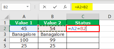
We can use the equal sign (=) to compare one cell value against the other cell value. In addition, we can compare all types of values using an equal sign. For example, assume we have the below values from cells A1 to B5.
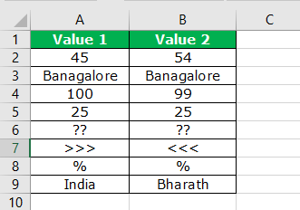
Now, we want to test whether the value in cell A1 is equal to cell B1’s value.
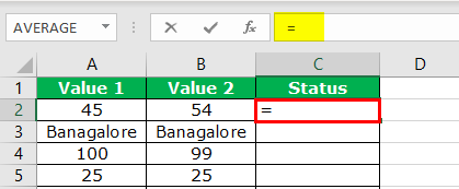
- To select the value of A1 to B1, let us open the formula with an equal sign.

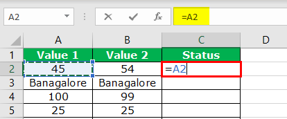
- Now, select cell A1.

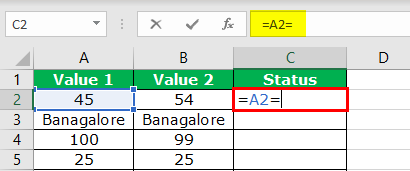
- Now, type the one more logical operator symbol equal sign (=).

- Now, select the second cell we are comparing, the B2 cell.

- Press the “Enter” key to close the formula. Then, we must copy and paste it into other cells.

So, we get “TRUE” as a result if the cell 1 value is equal to cell 2 or we get “FALSE.”
#2 Greater Than (>) Sign to Compare Numerical Values
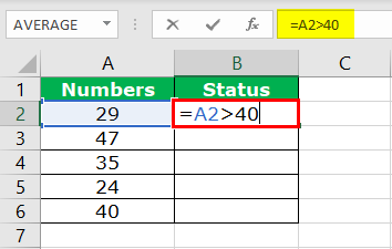
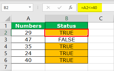
Unlike equal sign (=) greater than sign (>) can only test numerical values, not text values. So, for example, if the values are in cells A1 to A5 and we want to try whether these values are greater than (>) the value of 40 or not.

- Step 1: We must first open the formula in the B2 cell and select cell A2 as the cell reference.
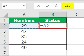
- Step 2: Since we are testing, the value is greater than the mention > symbol and apply the condition as 40.
- Step 3: Now, close the formula and use it to remain cells.
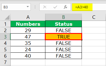
Only one value is >40, i.e., cell A3 value.
Cell A6 value is 40; since we have applied the logical operator > as the criteria formula returned, the result is FALSE. We will see how to solve this issue in the next example.
#3 Greater Than or Equal To (>=) Sign to Compare Numerical Values
In the previous example, the formula returns a TRUE value only to those greater than the criteria value. But if the criteria value is also included in the formula, we need to use the >= symbol.
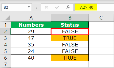
The previous formula excluded the value of 40, but this formula included.
#4 Less than Sign (<) to Compare Numerical Values
Like how greater than tests the numerical values are, similarly less than also tests the numbers. We have applied the formula as <40.
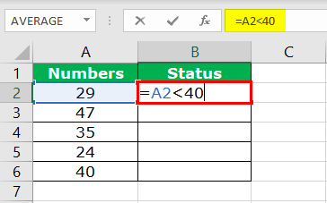
It works opposite to the greater than criteria. It has returned TRUE to all those values that are less than 40.

#5 Less Than or Equal To Sign (<=) to Compare Numerical Values
Like how >= sign includes the criteria value in the formula similarly, <= also performs the same way.
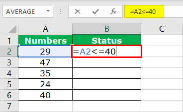
This formula had the criteria value, so the value of 40 is returned as TRUE.
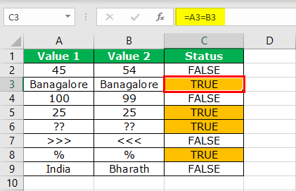
#6 Not Equal Sign (<>) to Compare Numerical Values
Combination of greater than (>) and less than (<) signs make the operator sign not equal to <>. It works opposite to an equal sign. The equal sign (=) tests whether the one value is equal to the other value and returns TRUE, whereas not equal to sign <> returns TRUE if the one value is not equal to another value and returns FALSE if the one value is not equal to another one.
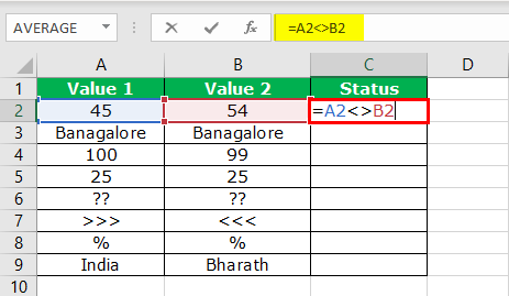
As we said, A3 and B3 cell values are the same, but the formula returns FALSE, which is completely different from the EQUAL sign logical operator.

Logical Operator in Excel with Formulas
We can also use logical operator symbols in other Excel formulas IF Excel function is one of the often used formulae with logical operators.
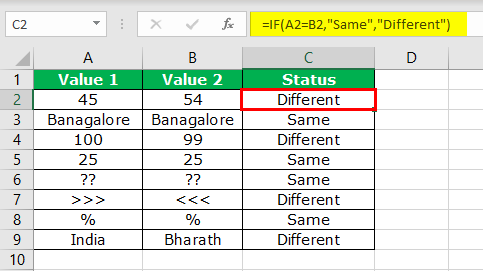
#1 – IF with Equal Sign
Suppose the function tests whether the condition is equal to a certain value or not. If the value is equal, then we can have our value. Below is a simple example of that.
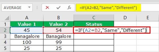
The formula returns the Same if the cell A2 value is equal to the B2 value; if not, it will return Different.
#2 – IF with Greater Than Sign
We can test certain numerical values, arrive at results if the condition is TRUE, and return a different result if the condition is FALSE.
#3 – IF with Less Than Sign
The below formula will show the logic of applying if with less than the logical operators.

Things to Remember
- Excel logical operator symbols return only TRUE or FALSE.
- Combination of > & < symbols do not equal sign <>.
- >= & <= sign includes the criteria also in the formula.
Recommended Articles
This article is a guide to Logical Operators in Excel. We discuss the top 6 types of MS Excel logical operators, practical examples, and a downloadable Excel template. You may learn more about Excel from the following articles: –
- How Not Equal to Works in Excel VBA?
- Greater Than or Equal to in Excel
- Divide Formula in Excel
- Multiply in Excel Formula
- Quotient in Excel
A lot of work in Excel involves comparing data in different cells. When you make a comparison between two values, you want to know one of these things:
- Is value A equal to value B (A=B)
- Is A greater than B (A>B)
- Is A less than B (A<B)
- Is A greater than or equal to B (A>=B)
- Is A less than or equal to B (A<=B)
- Is A not equal to B (A<>B)
These are called logical or boolean operators because there can only be two possible answers in any given case — TRUE or FALSE.
Using Logical Operators in your formulas
Excel is very flexible in the way that these logical operators can be used. For example, you can use them to compare two cells, or compare the results of one or more formulas. For example:
- =A1=A2
- =A1=(A2*5)
- =(A1*10)<=(A2/5)
As these examples suggest, you can type these directly into a cell in Excel and have Excel calculate the results of the formula just as it would do with any formula. With these formulas, Excel will always return either TRUE or FALSE as the result in the cell.
A common use of logical operators is found in Excel’s IF function (you can read more about the IF function here). The IF function works like this:
- =IF(logical_test,value_if_TRUE,value_if_FALSE)
In essence, the IF function carries out a logical test (the three examples above are all logical tests) and then return the appropriate result depending on whether the result of the test is true or false. For example:
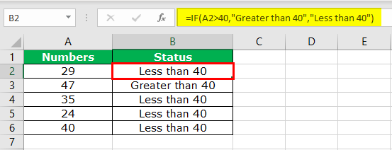
- =IF(A1>A2,»Greater than»,»Less than»)
- =IF(A1>A2,A1*10%,A1*5%)
However, you don’t always need to use an IF formula. Here’s a version of this formula that uses a logical operator, and also demonstrates another useful feature of logical operators in general:
- =(A1>A2)*(A1*10*)+(A1<=A2)*(A1*5%)
It looks confusing, but in fact it is very logical (excuse the pun). However, it helps to know that in Excel, TRUE is the same as 1, and FALSE is the same as 0.
So, in this example:
- If A1>A2 is TRUE, then the formula will multiple (A1*10%) by 1.
- Because A1>A2 is TRUE then A1<=A2 is false, so it will then multiply (A1*5%) by 0.
- It will then add the results together: (A1*10%)*1 + (A1*5%)*0.
- The final result is whatever (A1*10%) equals in the specific example.
Obviously, if A1 is less than A2, then the reverse of this would occur.
Using Multiple Logical Operators
In some cases, you may want to perform more than one comparison as part of your formula. For example:
- (Today is Wednesday) and (Sky is Blue)
- (Today is Wednesday) or (Sky is Blue)
- (Today is Wednesday and (Sky is NOT Blue)
- (Today is Wednesday) or (Sky is NOT Blue)
In Excel, you can use one of three logical functions to construct these formulas:
- AND
- OR
- NOT
The AND function works by performing multiple comparison tests and then returning TRUE if all of the tests were true, and FALSE if one or more of the tests were false. Here are a couple of examples:
- =AND(A1>A2,A1<A3) (if A1 is greater than A2 AND less than A3, then return TRUE otherwise return FALSE)
- IF(AND(A2>A2,A1<A3),»Both are true»,»At least one is false») (this IF function will return one of the two values depending on whether the AND function returns TRUE or FALSE).
The OR function works in a very similar way to the AND function. However, whereas AND requires that all tests return true, the OR function will return TRUE if only one of the tests return true. For example:
- =OR(A1>A2,A1<A3) (if either A1>A2 OR A1>A3 is true, then return TRUE. If neither are true, return FALSE).
- =IF(OR(A1>A2,A1<A3),»One or both are true»,»Neither are true»)
It is important to note that the AND and the IF functions can both incorporate up to 255 logical tests (my examples here have only used 2). Regardless of the number of tests you include, the same rules apply as they did in my simple examples.
It is also worth noting that you can combine the AND and OR functions in a single formula. For example:
- =AND(OR(A1>A2,A1<A3),A1>A4)
In this example, the AND function will only return TRUE if either (A1>A2 OR A1<A3) AND A1>A4
The final logical function you can use is the NOT function. The NOT function is somewhat self-explanatory — it takes any logical test result and does the opposite. For example:
- =(Sky is Blue) — will return TRUE if the sky is blue, and FALSE if the sky is not blue.
- =NOT(Sky is Blue) will return FALSE if the sky is blue, and TRUE if the sky is not blue.
Note that this example doesn’t care what other colors the sky might be!
Of course, you can use the NOT function with the AND, OR and IF functions:
- =NOT(AND(A1>A2,A1<A3)) — if A1>A2 AND A1<A3, then return FALSE
- =AND(NOT(A1>A2),A1<A3) — if A1 is NOT >A2 AND A1<A3 then return TRUE.
Note that writing NOT(A1>A2) is another way of writing (A1<=A2). In this simple example, using a NOT function didn’t add much value, but in some cases the NOT function can be very handy.
In summary, a lot of what you do in Excel, particularly once you start using IF functions, involves using logical operators. The logical functions, AND, OR and NOT are a great way to extend your use of logical operators to perform more complex calculations.
Как использовать функцию IF
Функция IF — это основная логическая функция в Excel, и поэтому она должна быть понятна первой. Он появится много раз на протяжении всей этой статьи.
Давайте посмотрим на структуру функции IF, а затем посмотрим несколько примеров ее использования.
Функция IF принимает 3 бита информации:
= IF (логический_тест, [value_if_true], [value_if_false])
- логический_тест: это условие для функции для проверки.
- value_if_true: действие, которое выполняется, если условие выполнено или является истинным.
- value_if_false: действие, которое нужно выполнить, если условие не выполнено или имеет значение false.
Операторы сравнения для использования с логическими функциями
При выполнении логического теста со значениями ячеек вы должны быть знакомы с операторами сравнения. Вы можете увидеть их в таблице ниже.

Теперь давайте посмотрим на некоторые примеры в действии.
Пример функции IF 1: текстовые значения
В этом примере мы хотим проверить, равна ли ячейка определенной фразе. Функция IF не учитывает регистр, поэтому не учитывает прописные и строчные буквы.
Следующая формула используется в столбце C для отображения «Нет», если столбец B содержит текст «Завершено» и «Да», если он содержит что-либо еще.
= ЕСЛИ (B2 = "Завершено", "Нет", "Да")

Хотя функция IF не чувствительна к регистру, текст должен точно соответствовать.
Пример функции IF 2: Числовые значения
Функция IF также отлично подходит для сравнения числовых значений.
В приведенной ниже формуле мы проверяем, содержит ли ячейка B2 число, большее или равное 75. Если это так, то мы отображаем слово «Pass», а если не слово «Fail».
= ЕСЛИ (В2> = 75, "Проход", "Сбой")

Функция IF — это намного больше, чем просто отображение разного текста в результате теста. Мы также можем использовать его для запуска различных расчетов.
В этом примере мы хотим предоставить скидку 10%, если клиент тратит определенную сумму денег. Мы будем использовать £ 3000 в качестве примера.
= ЕСЛИ (В2> = 3000, В2 * 90%, В2)

Часть формулы B2 * 90% позволяет вычесть 10% из значения в ячейке B2. Есть много способов сделать это.
Важно то, что вы можете использовать любую формулу в разделах value_if_true или value_if_false . И запускать различные формулы, зависящие от значений других ячеек, — очень мощный навык.
Пример функции IF 3: значения даты
В этом третьем примере мы используем функцию IF для отслеживания списка сроков исполнения. Мы хотим отобразить слово «Просрочено», если дата в столбце B уже в прошлом. Но если дата наступит в будущем, рассчитайте количество дней до даты исполнения.
Приведенная ниже формула используется в столбце C. Мы проверяем, меньше ли срок оплаты в ячейке B2, чем сегодняшний день (функция TODAY возвращает сегодняшнюю дату с часов компьютера).
= ЕСЛИ (В2 <СЕГОДНЯ (), "Просроченные", В2-СЕГОДНЯ ())

Что такое вложенные формулы IF?
Возможно, вы слышали о термине «вложенные IF» раньше. Это означает, что мы можем написать функцию IF внутри другой функции IF. Мы можем захотеть сделать это, если нам нужно выполнить более двух действий.
Одна функция IF способна выполнять два действия ( value_if_true и value_if_false ). Но если мы вставим (или вложим) другую функцию IF в раздел value_if_false , то мы можем выполнить другое действие.
Возьмите этот пример, где мы хотим отобразить слово «Отлично», если значение в ячейке B2 больше или равно 90, отобразить «Хорошо», если значение больше или равно 75, и отобразить «Плохо», если что-либо еще ,
= ЕСЛИ (В2> = 90, "Отлично", ЕСЛИ (В2> = 75, "Хорошо", "Плохо"))

Теперь мы расширили нашу формулу за пределы того, что может сделать только одна функция IF. И вы можете вложить больше функций IF, если это необходимо.
Обратите внимание на две закрывающие скобки в конце формулы — по одной для каждой функции IF.
Существуют альтернативные формулы, которые могут быть чище, чем этот вложенный подход IF. Одной из очень полезных альтернатив является функция SWITCH в Excel .
Логические функции AND и OR
Функции AND и OR используются, когда вы хотите выполнить более одного сравнения в своей формуле. Одна только функция IF может обрабатывать только одно условие или сравнение.
Возьмите пример, где мы дисконтируем значение на 10% в зависимости от суммы, которую тратит клиент, и сколько лет они были клиентом.
Сами функции AND и OR возвращают значение TRUE или FALSE.
Функция AND возвращает TRUE, только если выполняется каждое условие, а в противном случае возвращает FALSE. Функция OR возвращает TRUE, если выполняется одно или все условия, и возвращает FALSE, только если условия не выполняются.
Эти функции могут тестировать до 255 условий, поэтому они не ограничены только двумя условиями, как показано здесь.
Ниже приведена структура функций И и ИЛИ. Они написаны одинаково. Просто замените имя И на ИЛИ. Это просто их логика, которая отличается.
= И (логический1, [логический2] ...)
Давайте посмотрим на пример того, как они оба оценивают два условия.
Пример функции AND
Функция AND используется ниже, чтобы проверить, потратил ли клиент не менее 3000 фунтов стерлингов и был ли он клиентом не менее трех лет.
= И (В2> = 3000, С2> = 3)

Вы можете видеть, что он возвращает FALSE для Мэтта и Терри, потому что, хотя они оба соответствуют одному из критериев, они должны соответствовать обеим функциям AND.
Пример функции OR
Функция ИЛИ используется ниже, чтобы проверить, потратил ли клиент не менее 3000 фунтов стерлингов или был клиентом не менее трех лет.
= ИЛИ (В2> = 3000, С2> = 3)
В этом примере формула возвращает TRUE для Matt и Terry. Только Джули и Джиллиан не выполняют оба условия и возвращают значение FALSE.
Использование AND и OR с функцией IF
Поскольку функции И и ИЛИ возвращают значение ИСТИНА или ЛОЖЬ, когда используются по отдельности, они редко используются сами по себе.
Вместо этого вы обычно будете использовать их с функцией IF или внутри функции Excel, такой как условное форматирование или проверка данных, чтобы выполнить какое-либо ретроспективное действие, если формула имеет значение TRUE.
В приведенной ниже формуле функция AND вложена в логический тест функции IF. Если функция AND возвращает TRUE, тогда скидка 10% от суммы в столбце B; в противном случае скидка не предоставляется, а значение в столбце B повторяется в столбце D.
= ЕСЛИ (И (В2> = 3000, С2> = 3), В2 * 90%, В2)
Функция XOR
В дополнение к функции ИЛИ, есть также эксклюзивная функция ИЛИ. Это называется функцией XOR. Функция XOR была представлена в версии Excel 2013.
Эта функция может потребовать некоторых усилий, чтобы понять, поэтому практический пример показан.
Структура функции XOR такая же, как у функции OR.
= XOR (логический1, [логический2] ...)
При оценке только двух условий функция XOR возвращает:
- ИСТИНА, если любое условие оценивается как ИСТИНА.
- FALSE, если оба условия TRUE или ни одно из условий TRUE.
Это отличается от функции ИЛИ, потому что она вернула бы ИСТИНА, если оба условия были ИСТИНА.
Эта функция становится немного более запутанной, когда добавляется больше условий. Затем функция XOR возвращает:
- TRUE, если нечетное число условий возвращает TRUE.
- ЛОЖЬ, если четное число условий приводит к ИСТИНА, или если все условия ЛОЖЬ.
Давайте посмотрим на простой пример функции XOR.
В этом примере продажи делятся на две половины года. Если продавец продает 3000 и более фунтов стерлингов в обеих половинах, ему назначается Золотой стандарт. Это достигается с помощью функции AND с IF, как ранее в этой статье.
Но если они продают 3000 фунтов или более в любой половине, мы хотим присвоить им Серебряный статус. Если они не продают 3000 и более фунтов стерлингов в обоих случаях, то ничего.
Функция XOR идеально подходит для этой логики. Приведенная ниже формула вводится в столбец E и показывает функцию XOR с IF для отображения «Да» или «Нет», только если выполняется любое из условий.
= IF (XOR (В2> = 3000, С2> = 3000), "Да", "Нет")
Функция НЕ
Последняя логическая функция для обсуждения в этой статье — это функция NOT, и мы оставим самую простую последнюю. Хотя иногда поначалу бывает трудно увидеть использование этой функции в реальном мире.
Функция NOT меняет значение своего аргумента. Так что, если логическое значение ИСТИНА, тогда оно возвращает ЛОЖЬ. И если логическое значение ЛОЖЬ, оно вернет ИСТИНА.
Это будет легче объяснить на некоторых примерах.
Структура функции НЕ имеет вид;
= НЕ (логическое)
НЕ Функциональный Пример 1
В этом примере представьте, что у нас есть головной офис в Лондоне, а затем много других региональных сайтов. Мы хотим отобразить слово «Да», если на сайте есть что-то, кроме Лондона, и «Нет», если это Лондон.
Функция NOT была вложена в логический тест функции IF ниже, чтобы сторнировать ИСТИННЫЙ результат.
= ЕСЛИ (НЕ (B2 = "London"), "Да", "Нет")
Это также может быть достигнуто с помощью логического оператора NOT <>. Ниже приведен пример.
= ЕСЛИ (В2 <> "Лондон", "Да", "Нет")
НЕ Функциональный Пример 2
Функция NOT полезна при работе с информационными функциями в Excel. Это группа функций в Excel, которые что-то проверяют и возвращают TRUE, если проверка прошла успешно, и FALSE, если это не так.
Например, функция ISTEXT проверит, содержит ли ячейка текст, и вернет TRUE, если она есть, и FALSE, если нет. Функция NOT полезна, потому что она может отменить результат этих функций.
В приведенном ниже примере мы хотим заплатить продавцу 5% от суммы, которую он продает. Но если они ничего не перепродали, в ячейке есть слово «Нет», и это приведет к ошибке в формуле.
Функция ISTEXT используется для проверки наличия текста. Это возвращает TRUE, если текст есть, поэтому функция NOT переворачивает это на FALSE. И если ИФ выполняет свой расчет.
= ЕСЛИ (НЕ (ISTEXT (В2)), В2 * 5%, 0)
Овладение логическими функциями даст вам большое преимущество как пользователю Excel. Очень полезно иметь возможность проверять и сравнивать значения в ячейках и выполнять различные действия на основе этих результатов.
В этой статье рассматриваются лучшие логические функции, используемые сегодня. В последних версиях Excel появилось больше функций, добавленных в эту библиотеку, таких как функция XOR, упомянутая в этой статье. Будьте в курсе этих новых дополнений, вы будете впереди толпы.
There are many ways to add logical decision-making to your Excel spreadsheets. In addition to the standard logical operators in Excel (=, <, >, <>, <=, >=), Excel has compound logical functions which let you evaluate multiple conditions at once. The AND, OR, XOR, and NOT functions in Excel let you evaluate many logical conditions and simply return TRUE or FALSE depending on the function. Because they return TRUE or FALSE, these functions are commonly used with IF functions.
Excel AND Function
The AND function in Excel evaluates one or more logical conditions to determine whether ALL of them are true. It takes one or more conditions as its arguments separated by commas, and returns TRUE if ALL of the conditions are true. Otherwise, it returns FALSE.
=AND(condition_1, [condition_2], …)
The AND function only requires one argument, but can take more (up to 255). The arguments can be conditions, numbers and text, and cell references. If a cell reference argument is empty, the function simply ignores it. If an argument is a number, it will treat zero as FALSE and any non-zero number (even negatives) as TRUE.
=AND(1<2, «hello»<>»goodbye») evaluates to TRUE because both conditions are true: 1 is less than 2, and «hello» is not equal to «goodbye».
=AND(1<2, 0) returns FALSE because all arguments must be TRUE for the AND function to return true. While the first argument (1<2) is true, the second argument, 0, evaluates to FALSE, so the AND function must return FALSE.
Excel OR Function
The OR function in Excel evaluates one or more logical conditions to determine whether at least ONE of them is true. It takes one or more conditions as its arguments separated by commas and returns TRUE if at least one of the arguments is true. Otherwise, if all arguments are false, it returns FALSE.
=OR(condition_1, [condition_2], …)
The OR function requires only one argument but can take anywhere up to 255 in most versions of Excel. Like the AND function, the arguments can be conditions, numbers, cell references, even other AND/OR functions. If an argument is a number, it will treat zero as FALSE and any non-zero number as TRUE. It will also ignore blank cell references.
The OR function evaluates each argument and returns TRUE if at least one of the arguments is true.
=OR(1<2, 1) returns TRUE because both arguments are true. The first argument (1<2) is true, and Excel treats the number 1 as true because it is not zero.
=OR(1>2, 1) is also TRUE. The first argument (1>2) is false, but that’s okay because the second argument (1) is treated as TRUE because it’s not zero. As long as one of the arguments is true, OR will return true.
=OR(1>2, 0) will return FALSE because all of its arguments are false.
Excel XOR Function
The XOR function in Excel is the Exclusive OR function which, like the OR function, takes two conditions and evaluates whether one of them is true. But unlike the OR function, XOR returns TRUE if ONLY ONE argument is true. It returns FALSE if both arguments are true, or if both of the arguments are false. If XOR has more than two arguments, it returns TRUE if an ODD number of its arguments are TRUE, and FALSE if an EVEN number of its arguments are TRUE.
=XOR(condition_1, [condition_2], …)
The XOR function also only requires one argument but can take up to 255 in most recent versions of Excel. Like the AND and OR functions, it can take logical conditions, numbers, text, other logical functions, and cell references as its arguments. If a cell reference is blank, XOR will ignore it, and zero will be treated as FALSE while any non-zero number will be TRUE.
=XOR(1=1, «hello»=»goodbye») will return TRUE because only one argument is true. The first argument (1=1) is obviously true, but the second («hello»=»goodbye») is clearly false. Because only one argument is true, XOR returns TRUE.
=XOR(1=1, «hello» <> «goodbye») returns FALSE because multiple arguments are true. The first (1=1) is true, as is the second because «hello» is not equal to (<>) «goodbye» so XOR will return FALSE. XOR will only return TRUE if ONE of the arguments is true.
=XOR(1=2, «hello»=»goodbye») also returns FALSE because none of the arguments is true. The first (1=2) is false as is the second («hello»=»goodbye»).
Excel NOT Function
The NOT function in Excel is perhaps one of the most simple. It takes a single logical argument and returns TRUE or FALSE. It returns the opposite of the argument, so if the argument is true, NOT will return false, and if the argument is false, NOT will return true.
=NOT(condition)
=NOT(1=1) would return FALSE, because the argument is true.
=NOT(1=2) would return TRUE, because the argument is false.
The NOT function is particularly useful when you’re interested in excluding some property in Excel. For example, say you are looking at a spreadsheet of homes in Excel, and the B column contains the home’s city.
| A | B | C | D | E | |
|---|---|---|---|---|---|
| 1 | Home # | City | Price | ||
| 2 | Home 1 | Memphis | 300,000 | ||
| 3 | Home 2 | Minneapolis | 250,000 | ||
| 4 | Home 3 | Atlanta | 200,000 |
To exclude any homes in Minneapolis, you could write the following function (starting with row 2) and copy it all the way down the column:
=NOT(B2=»Minneapolis»)
This will return TRUE for any home where the city is not Minneapolis, so it will return true for Home 1 and Home 3, but will return false for Home 2.
Combining Logical Functions in Excel
Now imagine you only want to exclude single-family homes in Minneapolis, but keep other home types. City is still in column B, while home type is in column C.
=NOT(AND(B2=»Minneapolis», C2=»Single-Family»))
| A | B | C | D | E | |
|---|---|---|---|---|---|
| 1 | Home # | City | Home Type | ||
| 2 | Home 1 | Minneapolis | Apartment | ||
| 3 | Home 2 | Minneapolis | Single-Family | ||
| 4 | Home 3 | Atlanta | Single-Family |
Because the argument (an AND function) returns TRUE only for single-family homes in Minneapolis, this function will return TRUE for any home that is not a single-family home in Minneapolis. It will return true for Home 1 and Home 3, and will only return false for Home 2.
Combining XOR with AND in Excel
Suppose you love watching new movies, and your favorite movies were made after 2015. Suppose you also love movies that star Will Ferrell and John C. Reilly. But there’s a catch: You hate movies that star Will Ferrell and John C. Reilly that were made after 2015. In the table below, where column B is lead actor, column C is supporting actor, and column D is year, how would you find movies that were made after 2015, and movies with the two co-stars mentioned above, but not movies with the two co-stars made after 2015?
| A | B | C | D | |
|---|---|---|---|---|
| 1 | Title | Lead Actor | Supporting Actor | Year |
| 2 | Step Brothers | Will Ferrell | John C. Reilly | 2008 |
| 3 | Uncut Gems | Adam Sandler | Idina Menzel | 2019 |
| 4 | Anchorman | Will Ferrell | Christina Applegate | 2004 |
| 5 | Holmes & Watson | Will Ferrell | John C. Reilly | 2018 |
You could use the following formula:
=XOR(AND(B2=»Will Ferrell», C2=»John C. Reilly»), D2>2015)
Step Brothers: TRUE because AND(B2=»Will Ferrell», C2=»John C. Reilly») is TRUE while D2>2015 is FALSE.
Uncut Gems: TRUE because AND(B3=»Will Ferrell», C3=»John C. Reilly») is FALSE while D3>2015 is TRUE.
Anchorman: FALSE because both conditions: AND(B4=»Will Ferrell», C4=»John C. Reilly») as well as D4>2015 are FALSE
Holmes & Watson: FALSE because both conditions are true, thus it is a movie with Will Ferrell and John C. Reilly which was made after 2015.

Logical functions are some of the most popular and useful in Excel. They can test values in other cells and perform actions dependent upon the result of the test. This helps us to automate tasks in our spreadsheets.
How to Use the IF Function
The IF function is the main logical function in Excel and is, therefore, the one to understand first. It will appear numerous times throughout this article.
Let’s have a look at the structure of the IF function, and then see some examples of its use.
The IF function accepts 3 bits of information:
=IF(logical_test, [value_if_true], [value_if_false])
- logical_test: This is the condition for the function to check.
- value_if_true: The action to perform if the condition is met, or is true.
- value_if_false: The action to perform if the condition is not met, or is false.
Comparison Operators to Use with Logical Functions
When performing the logical test with cell values, you need to be familiar with the comparison operators. You can see a breakdown of these in the table below.

Now let’s look at some examples of it in action.
IF Function Example 1: Text Values
In this example, we want to test if a cell is equal to a specific phrase. The IF function is not case-sensitive so does not take upper and lower case letters into account.
The following formula is used in column C to display “No” if column B contains the text “Completed” and “Yes” if it contains anything else.
=IF(B2="Completed","No","Yes")
Although the IF function is not case sensitive, the text must be an exact match.
IF Function Example 2: Numeric Values
The IF function is also great for comparing numeric values.
In the formula below we test if cell B2 contains a number greater than or equal to 75. If it does, then we display the word “Pass,” and if not the word “Fail.”
=IF(B2>=75,"Pass","Fail")
The IF function is a lot more than just displaying different text on the result of a test. We can also use it to run different calculations.
In this example, we want to give a 10% discount if the customer spends a certain amount of money. We will use £3,000 as an example.
=IF(B2>=3000,B2*90%,B2)
The B2*90% part of the formula is a way that you can subtract 10% from the value in cell B2. There are many ways of doing this.
What’s important is that you can use any formula in the value_if_true or value_if_false sections. And running different formulas dependent upon the values of other cells is a very powerful skill to have.
IF Function Example 3: Date Values
In this third example, we use the IF function to track a list of due dates. We want to display the word “Overdue” if the date in column B is in the past. But if the date is in the future, calculate the number of days until the due date.
The formula below is used in column C. We check if the due date in cell B2 is less than today’s date (The TODAY function returns today’s date from the computer’s clock).
=IF(B2<TODAY(),"Overdue",B2-TODAY())
What are Nested IF Formulas?
You may have heard of the term nested IFs before. This means that we can write an IF function within another IF function. We may want to do this if we have more than two actions to perform.
One IF function is capable of performing two actions (the value_if_true and value_if_false ). But if we embed (or nest) another IF function in the value_if_false section, then we can perform another action.
Take this example where we want to display the word “Excellent” if the value in cell B2 is greater than or equal to 90, display “Good” if the value is greater than or equal to 75, and display “Poor” if anything else.
=IF(B2>=90,"Excellent",IF(B2>=75,"Good","Poor"))
We have now extended our formula to beyond what just one IF function can do. And you can nest more IF functions if necessary.
Notice the two closing brackets on the end of the formula—one for each IF function.
There are alternative formulas that can be cleaner than this nested IF approach. One very useful alternative is the SWITCH function in Excel.
The AND and OR functions are used when you want to perform more than one comparison in your formula. The IF function alone can only handle one condition, or comparison.
Take an example where we discount a value by 10% dependent upon the amount a customer spends and how many years they have been a customer.
On their own, the AND and OR functions will return the value of TRUE or FALSE.
The AND function returns TRUE only if every condition is met, and otherwise returns FALSE. The OR function returns TRUE if one or all of the conditions are met, and returns FALSE only if no conditions are met.
These functions can test up to 255 conditions, so are certainly not limited to just two conditions like is demonstrated here.
Below is the structure of the AND and OR functions. They are written the same. Just substitute the name AND for OR. It is just their logic which is different.
=AND(logical1, [logical2] ...)
Let’s see an example of both of them evaluating two conditions.
AND Function example
The AND function is used below to test if the customer spends at least £3,000 and has been a customer for at least three years.
=AND(B2>=3000,C2>=3)
You can see that it returns FALSE for Matt and Terry because although they both meet one of the criteria, they need to meet both with the AND function.
OR Function Example
The OR function is used below to test if the customer spends at least £3,000 or has been a customer for at least three years.
=OR(B2>=3000,C2>=3)
In this example, the formula returns TRUE for Matt and Terry. Only Julie and Gillian fail both conditions and return the value of FALSE.
Using AND and OR with the IF Function
Because the AND and OR functions return the value of TRUE or FALSE when used alone, it’s rare to use them by themselves.
Instead, you’ll typically use them with the IF function, or within an Excel feature such as Conditional Formatting or Data Validation to perform some retrospective action if the formula evaluates to TRUE.
In the formula below, the AND function is nested inside the IF function’s logical test. If the AND function returns TRUE then 10% is discounted from the amount in column B; otherwise, no discount is given and the value in column B is repeated in column D.
=IF(AND(B2>=3000,C2>=3),B2*90%,B2)
The XOR Function
In addition to the OR function, there is also an exclusive OR function. This is called the XOR function. The XOR function was introduced with the Excel 2013 version.
This function can take some effort to understand, so a practical example is shown.
The structure of the XOR function is the same as the OR function.
=XOR(logical1, [logical2] ...)
When evaluating just two conditions the XOR function returns:
- TRUE if either condition evaluates to TRUE.
- FALSE if both conditions are TRUE, or neither condition is TRUE.
This differs from the OR function because that would return TRUE if both conditions were TRUE.
This function gets a little more confusing when more conditions are added. Then the XOR function returns:
- TRUE if an odd number of conditions return TRUE.
- FALSE if an even number of conditions result in TRUE, or if all conditions are FALSE.
Let’s look at a simple example of the XOR function.
In this example, sales are split over two halves of the year. If a salesperson sells £3,000 or more in both halves then they are assigned Gold standard. This is achieved with an AND function with IF like earlier in the article.
But if they sell £3,000 or more in either half then we want to assign them Silver status. If they don’t sell £3,000 or more in both then nothing.
The XOR function is perfect for this logic. The formula below is entered into column E and shows the XOR function with IF to display “Yes” or “No” only if either condition is met.
=IF(XOR(B2>=3000,C2>=3000),"Yes","No")
The NOT Function
The final logical function to discuss in this article is the NOT function, and we have left the simplest for last. Although sometimes it can be hard to see the ‘real world’ uses of the function at first.
The NOT function reverses the value of its argument. So if the logical value is TRUE, then it returns FALSE. And if the logical value is FALSE, it will return TRUE.
This will be easier to explain with some examples.
The structure of the NOT function is;
=NOT(logical)
NOT Function Example 1
In this example, imagine we have a head office in London and then many other regional sites. We want to display the word “Yes” if the site is anything except London, and “No” if it is London.
The NOT function has been nested in the logical test of the IF function below to reverse the TRUE result.
=IF(NOT(B2="London"),"Yes","No")
This can also be achieved by using the NOT logical operator of <>. Below is an example.
=IF(B2<>"London","Yes","No")
NOT Function Example 2
The NOT function is useful when working with information functions in Excel. These are a group of functions in Excel that check something, and return TRUE if the check is a success, and FALSE if it is not.
For example, the ISTEXT function will check if a cell contains text and return TRUE if it does and FALSE if it does not. The NOT function is helpful because it can reverse the result of these functions.
In the example below, we want to pay a salesperson 5% of the amount they upsell. But if they did not upsell anything, the word “None” is in the cell and this will produce an error in the formula.
The ISTEXT function is used to check for the presence of text. This returns TRUE if there is text, so the NOT function reverses this to FALSE. And the IF performs its calculation.
=IF(NOT(ISTEXT(B2)),B2*5%,0)
Mastering logical functions will give you a big advantage as an Excel user. To be able to test and compare values in cells and perform different actions based on those results is very useful.
This article has covered the best logical functions used today. Recent versions of Excel have seen the introduction of more functions added to this library, such as the XOR function mentioned in this article. Keeping up to date with these new additions will keep you ahead of the crowd.
READ NEXT
- › How to Use an Advanced Filter in Microsoft Excel
- › Functions vs. Formulas in Microsoft Excel: What’s the Difference?
- › How to Use the IS Functions in Microsoft Excel
- › How to Use the IFS Function in Microsoft Excel
- › How to Use the IF Function in Microsoft Excel
- › How to Find the Function You Need in Microsoft Excel
- › 13 Essential Excel Functions for Data Entry
- › Google+ Will Come to a Final End on July 5, 2023