The IF function allows you to make a logical comparison between a value and what you expect by testing for a condition and returning a result if that condition is True or False.
-
=IF(Something is True, then do something, otherwise do something else)
But what if you need to test multiple conditions, where let’s say all conditions need to be True or False (AND), or only one condition needs to be True or False (OR), or if you want to check if a condition does NOT meet your criteria? All 3 functions can be used on their own, but it’s much more common to see them paired with IF functions.
Use the IF function along with AND, OR and NOT to perform multiple evaluations if conditions are True or False.
Syntax
-
IF(AND()) — IF(AND(logical1, [logical2], …), value_if_true, [value_if_false]))
-
IF(OR()) — IF(OR(logical1, [logical2], …), value_if_true, [value_if_false]))
-
IF(NOT()) — IF(NOT(logical1), value_if_true, [value_if_false]))
|
Argument name |
Description |
|
|
logical_test (required) |
The condition you want to test. |
|
|
value_if_true (required) |
The value that you want returned if the result of logical_test is TRUE. |
|
|
value_if_false (optional) |
The value that you want returned if the result of logical_test is FALSE. |
|
Here are overviews of how to structure AND, OR and NOT functions individually. When you combine each one of them with an IF statement, they read like this:
-
AND – =IF(AND(Something is True, Something else is True), Value if True, Value if False)
-
OR – =IF(OR(Something is True, Something else is True), Value if True, Value if False)
-
NOT – =IF(NOT(Something is True), Value if True, Value if False)
Examples
Following are examples of some common nested IF(AND()), IF(OR()) and IF(NOT()) statements. The AND and OR functions can support up to 255 individual conditions, but it’s not good practice to use more than a few because complex, nested formulas can get very difficult to build, test and maintain. The NOT function only takes one condition.

Here are the formulas spelled out according to their logic:
|
Formula |
Description |
|---|---|
|
=IF(AND(A2>0,B2<100),TRUE, FALSE) |
IF A2 (25) is greater than 0, AND B2 (75) is less than 100, then return TRUE, otherwise return FALSE. In this case both conditions are true, so TRUE is returned. |
|
=IF(AND(A3=»Red»,B3=»Green»),TRUE,FALSE) |
If A3 (“Blue”) = “Red”, AND B3 (“Green”) equals “Green” then return TRUE, otherwise return FALSE. In this case only the first condition is true, so FALSE is returned. |
|
=IF(OR(A4>0,B4<50),TRUE, FALSE) |
IF A4 (25) is greater than 0, OR B4 (75) is less than 50, then return TRUE, otherwise return FALSE. In this case, only the first condition is TRUE, but since OR only requires one argument to be true the formula returns TRUE. |
|
=IF(OR(A5=»Red»,B5=»Green»),TRUE,FALSE) |
IF A5 (“Blue”) equals “Red”, OR B5 (“Green”) equals “Green” then return TRUE, otherwise return FALSE. In this case, the second argument is True, so the formula returns TRUE. |
|
=IF(NOT(A6>50),TRUE,FALSE) |
IF A6 (25) is NOT greater than 50, then return TRUE, otherwise return FALSE. In this case 25 is not greater than 50, so the formula returns TRUE. |
|
=IF(NOT(A7=»Red»),TRUE,FALSE) |
IF A7 (“Blue”) is NOT equal to “Red”, then return TRUE, otherwise return FALSE. |
Note that all of the examples have a closing parenthesis after their respective conditions are entered. The remaining True/False arguments are then left as part of the outer IF statement. You can also substitute Text or Numeric values for the TRUE/FALSE values to be returned in the examples.
Here are some examples of using AND, OR and NOT to evaluate dates.

Here are the formulas spelled out according to their logic:
|
Formula |
Description |
|---|---|
|
=IF(A2>B2,TRUE,FALSE) |
IF A2 is greater than B2, return TRUE, otherwise return FALSE. 03/12/14 is greater than 01/01/14, so the formula returns TRUE. |
|
=IF(AND(A3>B2,A3<C2),TRUE,FALSE) |
IF A3 is greater than B2 AND A3 is less than C2, return TRUE, otherwise return FALSE. In this case both arguments are true, so the formula returns TRUE. |
|
=IF(OR(A4>B2,A4<B2+60),TRUE,FALSE) |
IF A4 is greater than B2 OR A4 is less than B2 + 60, return TRUE, otherwise return FALSE. In this case the first argument is true, but the second is false. Since OR only needs one of the arguments to be true, the formula returns TRUE. If you use the Evaluate Formula Wizard from the Formula tab you’ll see how Excel evaluates the formula. |
|
=IF(NOT(A5>B2),TRUE,FALSE) |
IF A5 is not greater than B2, then return TRUE, otherwise return FALSE. In this case, A5 is greater than B2, so the formula returns FALSE. |

Using AND, OR and NOT with Conditional Formatting
You can also use AND, OR and NOT to set Conditional Formatting criteria with the formula option. When you do this you can omit the IF function and use AND, OR and NOT on their own.
From the Home tab, click Conditional Formatting > New Rule. Next, select the “Use a formula to determine which cells to format” option, enter your formula and apply the format of your choice.

Using the earlier Dates example, here is what the formulas would be.

|
Formula |
Description |
|---|---|
|
=A2>B2 |
If A2 is greater than B2, format the cell, otherwise do nothing. |
|
=AND(A3>B2,A3<C2) |
If A3 is greater than B2 AND A3 is less than C2, format the cell, otherwise do nothing. |
|
=OR(A4>B2,A4<B2+60) |
If A4 is greater than B2 OR A4 is less than B2 plus 60 (days), then format the cell, otherwise do nothing. |
|
=NOT(A5>B2) |
If A5 is NOT greater than B2, format the cell, otherwise do nothing. In this case A5 is greater than B2, so the result will return FALSE. If you were to change the formula to =NOT(B2>A5) it would return TRUE and the cell would be formatted. |
Note: A common error is to enter your formula into Conditional Formatting without the equals sign (=). If you do this you’ll see that the Conditional Formatting dialog will add the equals sign and quotes to the formula — =»OR(A4>B2,A4<B2+60)», so you’ll need to remove the quotes before the formula will respond properly.
Need more help?

See also
You can always ask an expert in the Excel Tech Community or get support in the Answers community.
Learn how to use nested functions in a formula
IF function
AND function
OR function
NOT function
Overview of formulas in Excel
How to avoid broken formulas
Detect errors in formulas
Keyboard shortcuts in Excel
Logical functions (reference)
Excel functions (alphabetical)
Excel functions (by category)
Purpose
Test multiple conditions with AND
Return value
TRUE if all arguments evaluate TRUE; FALSE if not
Usage notes
The AND function is used to check more than one logical condition at the same time, up to 255 conditions, supplied as arguments. Each argument (logical1, logical2, etc.) must be an expression that returns TRUE or FALSE or a value that can be evaluated as TRUE or FALSE. The arguments provided to the AND function can be constants, cell references, arrays, or logical expressions.
The purpose of the AND function is to evaluate more than one logical test at the same time and return TRUE only if all results are TRUE. For example, if A1 contains the number 50, then:
=AND(A1>0,A1>10,A1<100) // returns TRUE
=AND(A1>0,A1>10,A1<30) // returns FALSE
The AND function will evaluate all values supplied and return TRUE only if all values evaluate to TRUE. If any value evaluates to FALSE, the AND function will return FALSE. Note: Excel will evaluate any number except zero (0) as TRUE.
Both the AND function and the OR function will aggregate results to a single value. This means they can’t be used in array operations that need to deliver an array of results. To work around this limitation, you can use Boolean logic. For more information, see: Array formulas with AND and OR logic.
Examples
To test if the value in A1 is greater than 0 and less than 5, you can use AND like this:
=AND(A1>0,A1<5)
You can embed the AND function inside the IF function. Using the above example, you can supply AND as the logical_test for the IF function like so:
=IF(AND(A1>0,A1<5), "Approved", "Denied")
This formula will return «Approved» only if the value in A1 is greater than 0 and less than 5.
You can combine the AND function with the OR function. The formula below returns TRUE when A1 > 100 and B1 is «complete» or «pending»:
=AND(A1>100,OR(B1="complete",B1="pending"))
See below for many more examples of how the AND function can be used.
Notes
- The AND function is not case-sensitive.
- The AND function does not support wildcards.
- Text values or empty cells supplied as arguments are ignored.
- The AND function will return #VALUE if no logical values are found or created during evaluation.
Things will not always be the way we want them to be. The unexpected can happen. For example, let’s say you have to divide numbers. Trying to divide any number by zero (0) gives an error. Logical functions come in handy such cases. In this tutorial, we are going to cover the following topics.
In this tutorial, we are going to cover the following topics.
- What is a Logical Function?
- IF function example
- Excel Logic functions explained
- Nested IF functions
What is a Logical Function?
It is a feature that allows us to introduce decision-making when executing formulas and functions. Functions are used to;
- Check if a condition is true or false
- Combine multiple conditions together
What is a condition and why does it matter?
A condition is an expression that either evaluates to true or false. The expression could be a function that determines if the value entered in a cell is of numeric or text data type, if a value is greater than, equal to or less than a specified value, etc.
IF Function example
We will work with the home supplies budget from this tutorial. We will use the IF function to determine if an item is expensive or not. We will assume that items with a value greater than 6,000 are expensive. Those that are less than 6,000 are less expensive. The following image shows us the dataset that we will work with.
 and conditions in Excel")
- Put the cursor focus in cell F4
- Enter the following formula that uses the IF function
=IF(E4<6000,”Yes”,”No”)
HERE,
- “=IF(…)” calls the IF functions
- “E4<6000” is the condition that the IF function evaluates. It checks the value of cell address E4 (subtotal) is less than 6,000
- “Yes” this is the value that the function will display if the value of E4 is less than 6,000
-
“No” this is the value that the function will display if the value of E4 is greater than 6,000
When you are done press the enter key
You will get the following results
 and conditions in Excel")
Excel Logic functions explained
The following table shows all of the logical functions in Excel
| S/N | FUNCTION | CATEGORY | DESCRIPTION | USAGE |
|---|---|---|---|---|
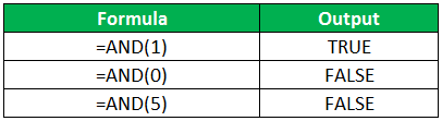
| 01 | AND | Logical | Checks multiple conditions and returns true if they all the conditions evaluate to true. | =AND(1 > 0,ISNUMBER(1)) The above function returns TRUE because both Condition is True. |
| 02 | FALSE | Logical | Returns the logical value FALSE. It is used to compare the results of a condition or function that either returns true or false | FALSE() |
| 03 | IF | Logical |
Verifies whether a condition is met or not. If the condition is met, it returns true. If the condition is not met, it returns false. =IF(logical_test,[value_if_true],[value_if_false]) |
=IF(ISNUMBER(22),”Yes”, “No”) 22 is Number so that it return Yes. |
| 04 | IFERROR | Logical | Returns the expression value if no error occurs. If an error occurs, it returns the error value | =IFERROR(5/0,”Divide by zero error”) |
| 05 | IFNA | Logical | Returns value if #N/A error does not occur. If #N/A error occurs, it returns NA value. #N/A error means a value if not available to a formula or function. |
=IFNA(D6*E6,0) N.B the above formula returns zero if both or either D6 or E6 is/are empty |
| 06 | NOT | Logical | Returns true if the condition is false and returns false if condition is true |
=NOT(ISTEXT(0)) N.B. the above function returns true. This is because ISTEXT(0) returns false and NOT function converts false to TRUE |
| 07 | OR | Logical | Used when evaluating multiple conditions. Returns true if any or all of the conditions are true. Returns false if all of the conditions are false |
=OR(D8=”admin”,E8=”cashier”) N.B. the above function returns true if either or both D8 and E8 admin or cashier |
| 08 | TRUE | Logical | Returns the logical value TRUE. It is used to compare the results of a condition or function that either returns true or false | TRUE() |
A nested IF function is an IF function within another IF function. Nested if statements come in handy when we have to work with more than two conditions. Let’s say we want to develop a simple program that checks the day of the week. If the day is Saturday we want to display “party well”, if it’s Sunday we want to display “time to rest”, and if it’s any day from Monday to Friday we want to display, remember to complete your to do list.
A nested if function can help us to implement the above example. The following flowchart shows how the nested IF function will be implemented.
 and conditions in Excel")
The formula for the above flowchart is as follows
=IF(B1=”Sunday”,”time to rest”,IF(B1=”Saturday”,”party well”,”to do list”))
HERE,
- “=IF(….)” is the main if function
- “=IF(…,IF(….))” the second IF function is the nested one. It provides further evaluation if the main IF function returned false.
Practical example
 and conditions in Excel")
Create a new workbook and enter the data as shown below
 and conditions in Excel")
- Enter the following formula
=IF(B1=”Sunday”,”time to rest”,IF(B1=”Saturday”,”party well”,”to do list”))
- Enter Saturday in cell address B1
- You will get the following results
 and conditions in Excel")
Download the Excel file used in Tutorial
Summary
Logical functions are used to introduce decision-making when evaluating formulas and functions in Excel.
На чтение 2 мин
Функция AND (И) в Excel используется для сравнения нескольких условий.
Содержание
- Что возвращает функция
- Синтаксис
- Аргументы функции
- Дополнительная информация
- Примеры использования функции AND (И, ИЛИ) в Excel
Что возвращает функция
Возвращает TRUE если значение или условие, при сравнении, соответствует критериям заданным в функции, или FALSE, в случае, если условие не соответствует критериям.
Синтаксис
=AND(logical1, [logical2],…) — английская версия
=И(логическое_значение1;[логическое_значение2];…) — русская версия
Аргументы функции
- logical1 (логическое_значение1) — первое условие, которое вы хотите оценить с помощью функции;
- [logical2] ([логическое_значение2]) (не обязательно) — второе условие, которое вы хотите оценить с помощью функции.
Дополнительная информация
- Функция может быть использована совместно с другими формулами;
- Например, с помощью функции IF (ЕСЛИ) вы можете проверить условие, а затем указать значение, когда оно TRUE, и значение, когда оно равно FALSE. Использование функции AND (И) вместе с функцией IF (ЕСЛИ) позволяет тестировать несколько условий за один раз;
Например, если вы хотите проверить значение в ячейке A1 на предмет того, больше оно чем «0» или меньше чем «100», то вы можете использовать следующую формулу:
=IF(AND(A1>0,A1<100),”Approve”,”Reject”) — английская версия
Больше лайфхаков в нашем Telegram Подписаться
=ЕСЛИ(И(A1>0;A1<100);»Одобрить»;»Против») — русская версия
- Аргументы функции должны быть логически вычислимы по принципу (TRUE/FALSE);
- Ячейки с пустыми или текстовыми значениями игнорируются функцией;
- Если в качестве аргументов функции не указаны логически вычислимые данные, то функция выдаст ошибку #VALUE!;
- Одновременно вы можете тестировать до 255 условий в рамках одного использования функции.
Примеры использования функции AND (И, ИЛИ) в Excel

The AND Function in excel is a logical function that tests multiple conditions and returns “true” or “false” depending on whether they are met or not. The formula of AND function is “=AND(logical1,[logical2]…),” where “logical1” is the first condition to evaluate.
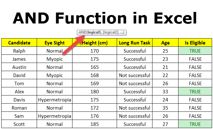
Table of contents
- AND Function in Excel
- Syntax of the AND Function
- The Characteristics of AND Function
- The Output of AND Function
- How to Use AND Function in Excel?
- Example #1–AND Function
- Example #2–AND Function With Nested IF Function
- Example #3–AND Function With Nested IF Function
- Nesting of AND Function in Excel
- Example #4–Nested AND Function
- Limitations of AND Function
- Frequently Asked Questions
- Recommended Articles
Syntax of the AND Function
The syntax is stated as follows:
The function accepts the following arguments:
- Logical 1: This is the first condition or logical value to evaluate.
- Logical 2: This is the second condition or logical value to evaluate.
The “logical 1” is a mandatory argument and “logical 2” is an optional argument.
The Characteristics of AND Function
- It returns “true” if all conditions or logical values evaluate to true.
- It returns “false” if any of the conditions or logical values evaluates to false.
- It can have more logical values depending on the situation and the requirement.
- It treats the value zero as “false” and all non-zero values as “true” while evaluating numbers.
- It ignores empty cells provided as an argument.
- It is often used in combination with other Excel functionsExcel functions help the users to save time and maintain extensive worksheets. There are 100+ excel functions categorized as financial, logical, text, date and time, Lookup & Reference, Math, Statistical and Information functions.read more like IF, OR, and so on.
The Output of AND Function
The output in different situations is given as follows:
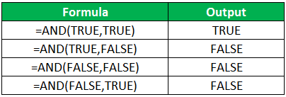
The output while evaluating numbers is given as follows:
How to Use AND Function in Excel?
It is easy to use the AND function. Let us understand its working with the help of a few examples.
You can download this AND Function Excel Template here – AND Function Excel Template
Example #1–AND Function
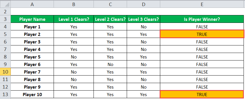
There are three levels and ten players in a game. To be a winner, a player has to clear all three levels. The player loses if he/she fails in any of the three levels.
The performance of the players in different levels is given in the following table. We are required to determine the winner.
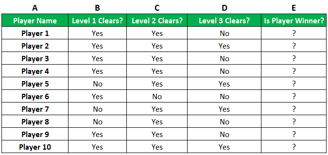
We apply AND formula in column E.
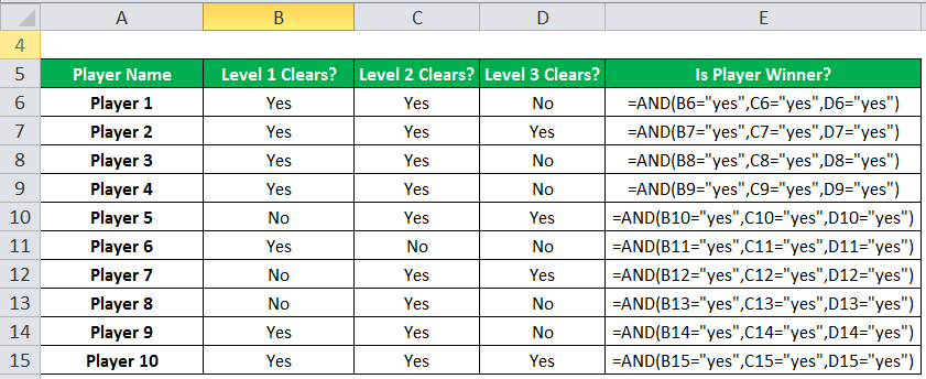
The output of the formula appears in column E.
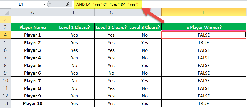
Player 2 and player 10 have cleared all the levels. Since all the logical conditions for these two players are met, the AND function gives the output “true.”
The rest of the players were unable to clear all three levels. If any of the levels is not cleared, the AND function returns “false.”
Example #2–AND Function With Nested IF Function
Let us consider the following example.
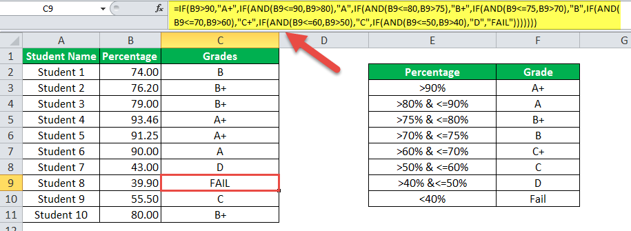
We have the marks (in percentage) of ten students in a school. We have to determine the grade obtained by each student according to the criteria given.
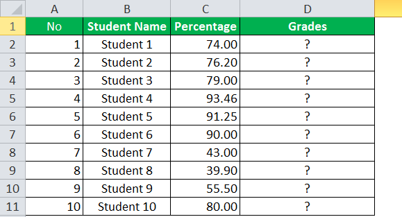
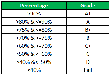
A student obtains “A+” if he/she scores more than 90%. If the percentage is greater than or equal to 80% but less than or equal to 90%, grade “A” is given.
If the percentage is less than 40%, the student fails. Likewise, the grades for the different percentages are given in the following table.
We apply the following formula.
“=IF(B2>90,”A+”,IF(AND(B2<=90,B2>80),”A”,IF(AND(B2<=80,B2>75),”B+”,IF(AND(B2<=75,B2>70),”B”,IF(AND(B2<=70,B2>60),”C+”,IF(AND(B2<=60,B2>50),”C”,IF(AND(B2<=50,B2>40),”D”,”FAIL”)))))))”
We use the nested IF functionIn Excel, nested if function means using another logical or conditional function with the if function to test multiple conditions. For example, if there are two conditions to be tested, we can use the logical functions AND or OR depending on the situation, or we can use the other conditional functions to test even more ifs inside a single if.read more with multiple AND functions to compute the grades. The latter allows testing two conditions together.
The syntax of the IF function is stated as follows:
“=IF(logical_test,[value_if_true],[value_if_false])”
The IF function returns “true” if the condition is met, else returns “false.”
The first logical test is “B2>90.” If this condition is “true,” grade “A+” is assigned. If this condition is “false,” the IF function evaluates the next condition.
The next logical testA logical test in Excel results in an analytical output, either true or false. The equals to operator, “=,” is the most commonly used logical test.read more is “B2<=90, B2>80.” If this condition is “true,” grade “A” is assigned. If this condition is “false,” the next statement is evaluated. Likewise, the IF function tests every condition given in the formula.
The last logical test is “B2<=50, B2>40.” If this condition is “true,” grade “D” is assigned, else the student fails.
We apply the formula to all categories of students, as shown in the following image.
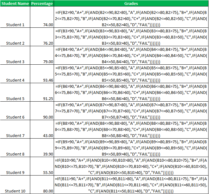
The output of the formula is shown in the succeeding image.
Example #3–AND Function With Nested IF Function
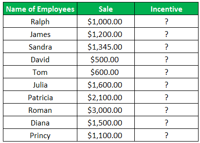
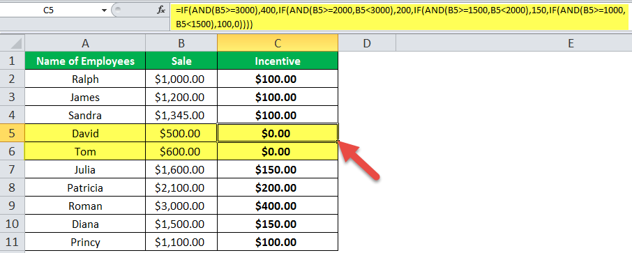
The name of employees and the sales revenueSales revenue refers to the income generated by any business entity by selling its goods or providing its services during the normal course of its operations. It is reported annually, quarterly or monthly as the case may be in the business entity’s income statement/profit & loss account.read more generated by them for an organization are shown in the succeeding image. Every employee is given a monetary incentive depending on the total sales made by him/her.
We have to calculate the incentives of all the employees based on their performance.
The incentive criteria followed by the organization is given in the succeeding table.
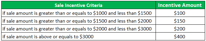
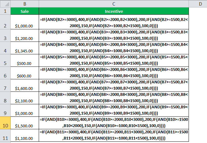
We apply the following formula.
“=IF(AND(B2>=3000),400,IF(AND(B2>=2000,B2<3000),200,IF(AND(B2>=1500,B2<2000),150,IF(AND(B2>=1000,B2<1500),100,0))))”
We use multiple IFs In Excel, multiple IF conditions are IF statements that are contained within another IF statement. They are used to test multiple conditions at the same time and return distinct values. Additional IF statements can be included in the ‘value if true’ and ‘value if false’ arguments of a standard IF formula.read moreand multiple AND functions to calculate the incentives received by all the employees, as shown in the following table.
Roman generates sales revenue of $3000. So, he receives an incentive amount of $400.
The revenue generated by David and Tom is $500 and $600, respectively. To be eligible for an incentive, minimum sales of $1000 is required. Hence, they do not get any incentive.
Nesting of AND Function in Excel
A nested function refers to using a function inside another Excel function. In Excel, the nesting of functions up to 64 levels is allowed.
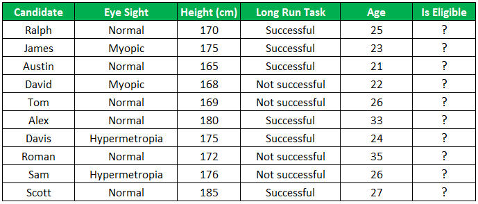
Example #4–Nested AND Function
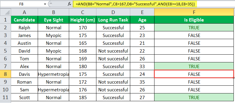
We have a list of candidates who wish to join the Army subject to certain conditions. The eligibility criteria are stated as follows:
- The age should be greater than or equal to 18, but less than 35 years.
- The height should be greater than 167 cm.
- The eyesight should be normal.
- The candidate must have completed the long-run task.
We need to find out the candidates who are eligible for joining the Army.
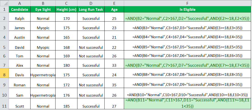
To evaluate the candidates on the given parameters, we use the nested AND function.
We apply the following formula.
“=AND(B2=”Normal”,C2>167,D2=”Successful”,AND(E2>=18,E2<35))”
We evaluate multiple logical conditions simultaneously. We also check whether the age is within the prescribed limit or not. So, we use the AND function inside another AND function.
The output of the formula is shown in the succeeding image.
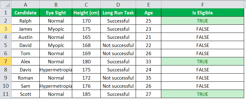
The candidates Ralph, Alex, and Scott pass the selection criteria. Hence, their eligibility output (in column F) is “true.” The remaining candidates are not eligible for joining the Army.
Limitations of AND Function
The limitations are listed as follows:
- With Excel 2007 onwards, the AND function can test up to 255 arguments given that the length of the formula does not exceed 8,162 characters.
- In Excel 2003 and previous versions, the AND function can test up to 30 arguments given that the length of the formula does not exceed 1,024 characters.
- The AND function returns “#VALUE! error#VALUE! Error in Excel represents that the reference cell the user has either entered an incorrect formula or used a wrong data type (mostly numerical data). Sometimes, it is difficult to identify the kind of mistake behind this error.read more” if logical conditions are passed as text or if none of the arguments evaluates to a logical value.
- The AND function returns “#VALUE! error” if all the arguments provided are empty cells.
The following two images show the output of the AND function when an empty cell and a text string is provided as an argument.

Frequently Asked Questions
#1 – When should the AND function of Excel be used
#2 – How is the AND function used with the OR function in Excel?
The OR function helps compare two values or statements. The AND function is combined with the OR function by the following formulas:
“=AND(OR(Condition1,Condition2),Condition3)”
“=AND(OR(Condition1,Condition2),OR(Condition3,Condition4)”
“=OR(AND(Condition1,Condition2),Condition3)”
“=OR(AND(Condition1,Condition2),AND(Condition3,Condition4))”
#3 – What is the difference between AND, IF, and OR functions in Excel?
The difference between the three functions is stated as follows:
– The AND function helps evaluate multiple conditions at the same time. It returns “true” when all conditions are true; otherwise, it returns “false.”
– The IF function helps compare the value with the result expected by the user. It returns specific values for the “true” and “false” outcomes.
– The OR function helps compare two values or two statements. It returns “true” when at least one of the specified conditions is met. It returns “false” if all the logical values evaluate to false.
- The AND function tests multiple conditions and returns “true” or “false” depending upon whether they are met or not.
- The AND function returns “true” if all conditions evaluate to true and returns “false” if any of the conditions evaluates to false.
- The AND function treats the value zero as “false.”
- The AND function can test up to 255 arguments in the latest versions of Excel.
- The AND function returns “#VALUE! error” if logical conditions are passed as a text.
- The formula of the IF function is “=IF(logical_test,[value_if_true],[value_if_false]).”
Recommended Articles
This has been a guide to AND Function in Excel. Here we discuss how to use AND Formula in Excel along with examples and downloadable excel templates. You may also look at these useful functions in Excel –
- Excel Pivot Table Add ColumnThe pivot table add column helps to add a new column in a pivot table.read more
- Excel Convert FunctionAs the word itself, the Excel CONVERT function defines that it can convert the numbers from one measurement system to another measurement system.read more
- VBA Boolean Data TypeBoolean is an inbuilt data type in VBA used for logical references or logical variables. The value this data type holds is either TRUE or FALSE and is used for logical comparison. The declaration of this data type is similar to all the other data types.read more
- IF AND Formula in ExcelThe IF AND excel formula is the combination of two different logical functions often nested together that enables the user to evaluate multiple conditions using AND functions. Based on the output of the AND function, the IF function returns either the “true” or “false” value, respectively.
read more
Excel IF AND OR functions on their own aren’t very exciting, but mix them up with the IF Statement and you’ve got yourself a formula that’s much more powerful.
In this tutorial we’re going to take a look at the basics of the AND and OR functions and then put them to work with an IF Statement. If you aren’t familiar with IF Statements, click here to read that tutorial first.
IF Formula Builder
Our IF Formula Builder does the hard work of creating IF formulas.
You just need to enter a few pieces of information, and the workbook creates the formula for you.
AND Function
The AND function belongs to the logic family of formulas, along with IF, OR and a few others. It’s useful when you have multiple conditions that must be met.
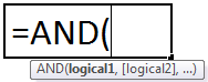
In Excel language on its own the AND formula reads like this:
=AND(logical1,[logical2]....)
Now to translate into English:
=AND(is condition 1 true, AND condition 2 true (add more conditions if you want)
OR Function
The OR function is useful when you are happy if one, OR another condition is met.
In Excel language on its own the OR formula reads like this:
=OR(logical1,[logical2]....)
Now to translate into English:
=OR(is condition 1 true, OR condition 2 true (add more conditions if you want)
See, I did say they weren’t very exciting, but let’s mix them up with IF and put AND and OR to work.
IF AND Formula
First let’s set the scene of our challenge for the IF, AND formula:
In our spreadsheet below we want to calculate a bonus to pay the children’s TV personalities listed. The rules, as devised by my 4 year old son, are:
1) If the TV personality is Popular AND
2) If they earn less than $100k per year they get a 10% bonus (my 4 year old will write them an IOU, he’s good for it though).

In cell D2 we will enter our IF AND formula as follows:
In English first
=IF(Spider Man is Popular, AND he earns <$100k), calculate his salary x 10%, if not put "Nil" in the cell)
Now in Excel’s language:
=IF(AND(B2="Yes",C2<100),C2x$H$1,"Nil")
You’ll notice that the two conditions are typed in first, and then the outcomes are entered. You can have more than two conditions; in fact you can have up to 30 by simply separating each condition with a comma (see warning below about going overboard with this though).
IF OR Formula
Again let’s set the scene of our challenge for the IF, OR formula:
The revised rules, as devised by my 4 year old son, are:
1) If the TV personality is Popular OR
2) If they earn less than $100k per year they get a 10% bonus.

In cell D2 we will enter our IF OR formula as follows:
In English first
=IF(Spider Man is Popular, OR he earns <$100k), calculate his salary x 10%, if not put “Nil” in the cell)
Now in Excel’s language:
=IF(OR(B2="Yes",C2<100),C2x$H$1,"Nil")
Notice how a subtle change from the AND function to the OR function has a significant impact on the bonus figure.
Just like the AND function, you can have up to 30 OR conditions nested in the one formula, again just separate each condition with a comma.
Try other operators
You can set your conditions to test for specific text, as I have done in this example with B2=»Yes», just put the text you want to check between inverted comas “ ”.
Alternatively you can test for a number and because the AND and OR functions belong to the logic family, you can employ different tests other than the less than (<) operator used in the examples above.
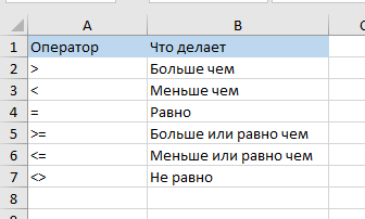
Other operators you could use are:
- = Equal to
- > Greater Than
- <= Less than or equal to
- >= Greater than or equal to
- <> Less than or greater than
Warning: Don’t go overboard with nesting IF, AND, and OR’s, as it will be painful to decipher if you or someone else ever needs to update the formula in months or years to come.
Note: These formulas work in all versions of Excel, however versions pre Excel 2007 are limited to 7 nested IF’s.
Download the Workbook
Enter your email address below to download the sample workbook.
By submitting your email address you agree that we can email you our Excel newsletter.
Excel IF AND OR Practice Questions
IF AND Formula Practice
In the embedded Excel workbook below insert a formula (in the grey cells in column E), that returns the text ‘Yes’, when a product SKU should be reordered, based on the following criteria:
- If Stock on hand is less than 20,000 AND
- Demand level is ‘High’
If the above conditions are met, return ‘Yes’, otherwise, return ‘No’.
Tips for working with the embedded workbook:
- Use arrow keys to move around the worksheet when you can’t click on the cells with your mouse
- Use shortcut keys CTRL+C to copy and CTRL+V to paste
- Don’t forget to absolute cell references where applicable
- Do not enter anything in column F
- Double click to edit a cell
- Refresh the page to reset the embedded workbook
IF OR Formula Practice
In the embedded Excel workbook below insert a formula (in the grey cells in column E) that calculates the bonus due for each salesperson. A $500 bonus is paid if a salesperson meets either target in cells C24 and C25, otherwise they earn $0 bonus.
Want More Excel Formulas
Why not visit our list of Excel formulas. You’ll find a huge range all explained in plain English, plus PivotTables and other Excel tools and tricks. Enjoy 🙂
To write an IF, AND, OR array formula in Excel 365, we must use the arithmetic operators * (multiplication) and + (addition). Why it’s so?
If we take the logical AND, OR with the IF in Excel 365 to spill the result, we won’t get our expected result.
I mean, such a formula won’t support a range/array in evaluation. Even if it supports, it won’t return an array result.
So we will replace the AND logical operator with the * (multiplication) and OR with the + (addition) arithmetic operators.
Coding the formula with the said two operators is very simple and easily readable.
I think I can convince you the same with the examples below.
Example to IF, AND, OR in Excel 365 (Non-Array Formula)
Imagine a user played a game three times, and we have recorded his scores out of 100 in cells A2, B2, and C2.
We want to perform the following three logical tests on the scores individually.
- If all scores are >=80, return OK.
- If any of the two scores are >=80, return OK.
- Finally, if any of the scores is >=80, return OK.
Logical Tests Using IF, AND, OR Functions
In Excel, we can perform the above three logical tests as follows.
1. E2 (If all scores are >=80, return OK)
=IF(AND(A2>=80,B2>=80,C2>=80),"OK","NOT OK")I have used the AND function with IF in the above Excel formula to test if all the three logical tests return TRUE.
2. F2 (If any of the two scores are >=80, return OK)
We must use the following logic (two parts) to test if any two logical tests return TRUE.
AND Part:-
a) Value 1>=80 and value 2>=80.
b) Value 1>=80 and value 3>=80.
c) Value 2>=80 and value 3>=80.
OR Part:-
a) The OR evaluates to TRUE if any two of the above three AND tests return TRUE.
So the formula will be as follows.
=IF(OR(AND(A2>=80,B2>=80),AND(A2>=80,C2>=80),AND(B2>=80,C2>=80)),"OK","NOT OK")It is an example of the IF, AND, OR logical test in Excel.
3. G2 (if any of the scores is >=80, return OK)
=IF(OR(A2>=80,B2>=80,C2>=80),"OK","NOT OK")Here I have used the OR function with IF to test if any of the three logical tests return TRUE.
As I have already mentioned, we can’t write an IF, AND, OR array formula as above in Excel 365.
Logical Tests Using IF, *, + Formula
Let’s substitute the above three formulas by replacing AND, OR with multiplication and addition.
But that’s not enough. Then?
The below formulas are self-explanatory.
1. E2 Formula
=IF((A2:A8>=80)*(B2:B8>=80)*(C2:C8>=80),"OK","NOT OK")How the multiplication replaces the logical function OR above?
Each test in the formula returns either TRUE or FALSE. If all the criteria are met, it will be =IF((TRUE*TRUE*TRUE),"OK","NOT OK").
We can even replace the multiplication operator here with addition.
=IF((A2:A8>=80)+(B2:B8>=80)+(C2:C8>=80)>2,"OK","NOT OK")Please remember that the value of TRUE is 1, and FALSE is 0.
2. F2 Formula
=IF((A2:A8>=80)+(B2:B8>=80)+(C2:C8>=80)>1,"OK","NOT OK")3. G2 Formula
=IF((A2:A8>=80)+(B2:B8>=80)+(C2:C8>=80)>0,"OK","NOT OK")Above I have tried to simplify the use of the logical operators within the IF function.
Now let’s open an Excel Spreadsheet and enter the scores of multiple players in the range A2:C8 as below.

So the values to evaluate are in cell range A2:C8.
I have inserted the following three IF, AND, OR array formulas in cells E2, F2, and G2, respectively.
1. E2 Array Formula
=IF((A2:A8>=80)*(B2:B8>=80)*(C2:C8>=80),"OK","NOT OK")2. F2 Array Formula
=IF((A2:A8>=80)+(B2:B8>=80)+(C2:C8>=80)>1,"OK","NOT OK")3. G2 Array Formula
=IF((A2:A8>=80)+(B2:B8>=80)+(C2:C8>=80)>0,"OK","NOT OK")If any of the above formulas return #SPILL!, please empty the cells down in that column.
Nested IF, AND, OR Combination in Excel 365
I want to assign grades based on the scores above.
In that case, we may require to write a nested IF, AND, OR combination array formula in Excel 365.
Here is how.
In the above example, we have used three formulas for the below three logical tests.
- If all scores are >=80, return OK.
- If any of the two scores are >=80, return OK.
- Finally, if any of the scores is >=80, return OK.
There each test returns OK or NOT OK.
Instead of that, here, I want the tests to return GR-1, GR-2, and GR-3.
- If all scores are >=80, return GR-1.
- If any of the two scores are >=80, return GR-2.
- Finally, if any of the scores is >=80, return GR-3.
For that, we should combine the above three IF, AND, OR Array Formulas.
How?
In the E2 formula, replace “OK” with “GR-1” and “NOT OK” with the F2 formula.
In that combined (E2 and F2) formula, replace “OK” with “GR-2” and “NOT OK” with the G2 formula.
Then, in the combined E2, F2, and G2 formula, replace “OK” with “GR-3” and replace “NOT OK” with “F.”
Here it is.

=IF(
     (A2:A8>=80)*(B2:B8>=80)*(C2:C8>=80),"GR-1",
     IF(
        (A2:A8>=80)+(B2:B8>=80)+(C2:C8>=80)>1,"GR-2",
        IF(
           (A2:A8>=80)+(B2:B8>=80)+(C2:C8>=80)>0,"GR-3","F"
        )
     )
)
We can call it a nested IF, AND, OR combination array formula.
Related:- How to Use the IFS Function in Excel 365.
The logical IF statement in Excel is used for the recording of certain conditions. It compares the number and / or text, function, etc. of the formula when the values correspond to the set parameters, and then there is one record, when do not respond — another.
Logic functions — it is a very simple and effective tool that is often used in practice. Let us consider it in details by examples.
The syntax of the function «IF» with one condition
The operation syntax in Excel is the structure of the functions necessary for its operation data.
=IF(boolean;value_if_TRUE;value_if_FALSE)
Let us consider the function syntax:
- Boolean – what the operator checks (text or numeric data cell).
- Value_if_TRUE – what will appear in the cell when the text or numbers correspond to a predetermined condition (true).
- Value_if_FALSE – what appears in the box when the text or the number does not meet the predetermined condition (false).
Example:

Logical IF functions.
The operator checks the A1 cell and compares it to 20. This is a «Boolean». When the contents of the column is more than 20, there is a true legend «greater 20». In the other case it’s «less or equal 20».
Attention! The words in the formula need to be quoted. For Excel to understand that you want to display text values.
Here is one more example. To gain admission to the exam, a group of students must successfully pass a test. The results are listed in a table with columns: a list of students, a credit, an exam.

The statement IF should check not the digital data type but the text. Therefore, we prescribed in the formula В2= «done» We take the quotes for the program to recognize the text correctly.
The function IF in Excel with multiple conditions
Usually one condition for the logic function is not enough. If you need to consider several options for decision-making, spread operators’ IF into each other. Thus, we get several functions IF in Excel.
The syntax is as follows:
Here the operator checks the two parameters. If the first condition is true, the formula returns the first argument is the truth. False — the operator checks the second condition.
Examples of a few conditions of the function IF in Excel:

It’s a table for the analysis of the progress. The student received 5 points:
- А – excellent;
- В – above average or superior work;
- C – satisfactory;
- D – a passing grade;
- E – completely unsatisfactory.
IF statement checks two conditions: the equality of value in the cells.

In this example, we have added a third condition, which implies the presence of another report card and «twos». The principle of the operator is the same.
Enhanced functionality with the help of the operators «AND» and «OR»
When you need to check out a few of the true conditions you use the function И. The point is: IF A = 1 AND A = 2 THEN meaning в ELSE meaning с.
OR function checks the condition 1 or condition 2. As soon as at least one condition is true, the result is true. The point is: IF A = 1 OR A = 2 THEN value B ELSE value C.
Functions AND & OR can check up to 30 conditions.
An example of using the operator AND:

It’s the example of using the logical operator OR.

How to compare data in two tables
Users often need to compare the two spreadsheets in an Excel to match. Examples of the «life»: compare the prices of goods in different bringing, to compare balances (accounting reports) in a few months, the progress of pupils (students) of different classes, in different quarters, etc.
To compare the two tables in Excel, you can use the COUNTIFS statement. Consider the order of application functions.
For example, consider the two tables with the specifications of various food processors. We planned allocation of color differences. This problem in Excel solves the conditional formatting.
Baseline data (tables, which will work with):

Select the first table. Conditional Formatting — create a rule — use a formula to determine the formatted cells:

In the formula bar write: = COUNTIFS (comparable range; first cell of first table)=0. Comparing range is in the second table.
To drive the formula into the range, just select it first cell and the last. «= 0» means the search for the exact command (not approximate) values.
Choose the format and establish what changes in the cell formula in compliance. It’s better to do a color fill.
Select the second table. Conditional Formatting — create a rule — use the formula. Use the same operator (COUNTIFS). For the second table formula:
Download all examples in Excel

Now it is easy to compare the characteristics of the data in the table.
На чтение 3 мин Просмотров 3.4к. Опубликовано 07.12.2021
Эта функция проверяет, правильно ли заданное в аргументах утверждение, если да то выполняет указанное действие. Например, можно просто вывести ИСТИНА или ЛОЖЬ.
Содержание
- Результат функции
- Формула
- Аргументы функции
- Важная информация
- Примеры
- Проверяем соответствует ли число заданным критериям с помощью функции ЕСЛИ в Excel
- Проверяем сразу несколько критериев
- Вычисляем комиссию
- Пример 4: Использование логических операторов (AND/OR) в функции IF в Excel
- Как убрать ошибки при использовании функции ЕСЛИ в Excel
Результат функции
Результатом функции будет указанное вами значение, указать это самое значение можно для двух исходов(истина или ложь)
Формула
=ЕСЛИ(проверяемый_аргумент; значение_если_истина; значение_если_ложь)
Аргументы функции
- проверяемый аргумент — аргумент, который, в результате выполнения функции, будет проверен. Результатом будет ИСТИНА либо ЛОЖЬ;
- значение_если_истина — значение, которое вернет функция ЕСЛИ в случае, если проверяемый аргумент оказался истиной.
- значение_если_ложь — значение, которое вернет функция ЕСЛИ в случае, если проверяемый аргумент оказался ложью.
Важная информация
- Максимум проверяемых аргументов может быть 64;
- В случае, когда вы используете функцию для проверки каких-либо условий относительно массива, будет проверено каждое значение этого самого массива;
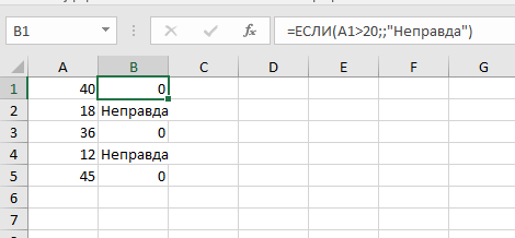
- Если вместо аргумента вы оставите пустое место, результатом выполнения функции будет 0, то есть.
На картинке ниже, мы оставили пустое место для значения, которое будет результатом, если проверяемый аргумент оказался ложью:
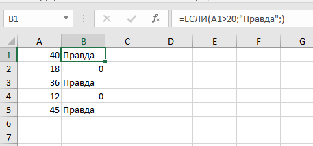
Тоже самое, но для аргумента «Истины»:
Примеры
Итак, давайте рассмотрим различные ситуации.
Проверяем соответствует ли число заданным критериям с помощью функции ЕСЛИ в Excel
В проверяемом аргументе функции, при работе с обычными числами, вы указываете оператор(или операторы) чтобы проверить, соответствует ли число каким-либо критериям. Вот список этих операторов:

Сразу же рассмотрим такую ситуацию:
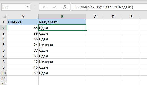
Если число в столбце A больше либо равно 35, то результатом выполнения функции будет «Сдал», если же нет, то «Не сдал».
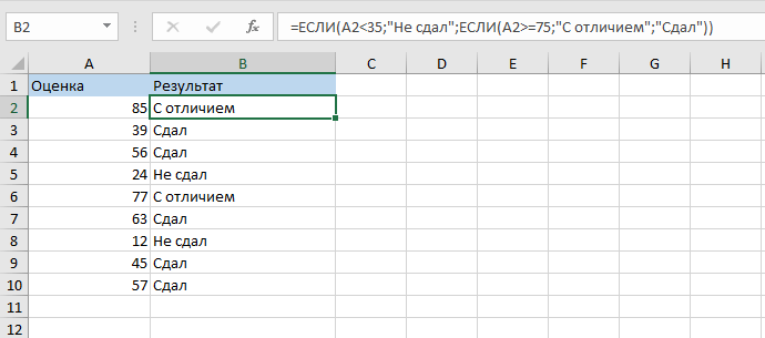
Проверяем сразу несколько критериев
Итак, давайте рассмотрим ситуацию, когда вам нужно проверить, соответствует ли число сразу нескольким критериям. Мы помним, что максимальное число проверяемых аргументов — 64. Давайте попробуем проверить хотя бы 2 критерия.
В приведенном ниже примере мы проверяем два условия.
- Меньше ли значение в ячейке чем число 35;
- В случае, когда в результате первой проверки возвращается ЛОЖЬ, проверяется больше или равно значение в ячейке чем число 75.
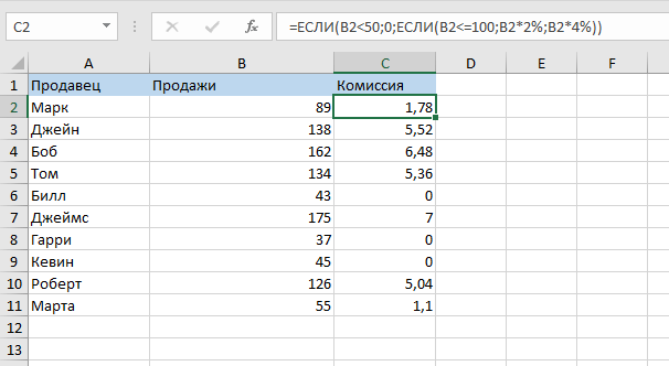
Вычисляем комиссию
Итак, с помощью этой функции мы можем даже посчитать комиссию, которую забирает себе конкретный продавец.
В ситуации описанной ниже, продавец не получает комиссию, если у него меньше 50-ти продаж. Если первое проверочное условие он прошел, тогда проверяем второе. Если у продавца меньше 100 продаж, его комиссия будет продажи*2%, а если больше, то — продажи*4%
Пример 4: Использование логических операторов (AND/OR) в функции IF в Excel
Также, мы можем использовать функции И и ИЛИ для проверки по сразу нескольким критериям.
Допустим, как указано на картинке ниже, мы имеем такую табличку:
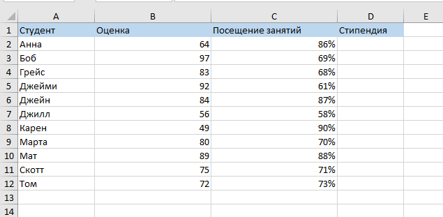
Наша задача — рассчитать у кого из студентов будет стипендия. Данные для выдачи стипендии будут сразу же в формуле:
=ЕСЛИ(И(B2>80;C2>80%); "Да"; "Нет")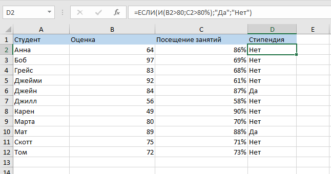
Как убрать ошибки при использовании функции ЕСЛИ в Excel
Теперь давайте разберемся как мы можем фильтровать ошибки при использовании функции.
Формула:
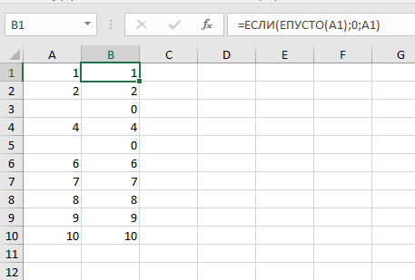
=ЕСЛИ(ЕСЛИОШИБКА(A1);0;A1)Теперь, если в результате выполнения функции мы получим ошибку, она будет отфильтрована и превращена в 0. А если ошибки не произойдет — мы просто получим значение.
Точно также можно использовать функцию ЕПУСТО:
=ЕСЛИ(ЕПУСТО(A1);0;A1)