
Excel for Microsoft 365 Excel for Microsoft 365 for Mac Excel for the web Excel 2021 Excel 2021 for Mac Excel 2019 Excel 2019 for Mac Excel 2016 Excel 2016 for Mac Excel 2013 Excel 2010 Excel 2007 Excel for Mac 2011 Excel Starter 2010 More…Less
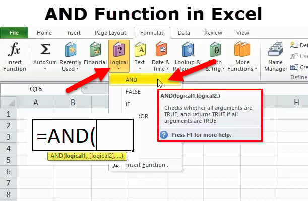
Use the AND function, one of the logical functions, to determine if all conditions in a test are TRUE.
Example
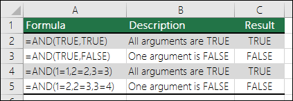
The AND function returns TRUE if all its arguments evaluate to TRUE, and returns FALSE if one or more arguments evaluate to FALSE.
One common use for the AND function is to expand the usefulness of other functions that perform logical tests. For example, the IF function performs a logical test and then returns one value if the test evaluates to TRUE and another value if the test evaluates to FALSE. By using the AND function as the logical_test argument of the IF function, you can test many different conditions instead of just one.
Syntax
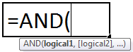
AND(logical1, [logical2], …)
The AND function syntax has the following arguments:
|
Argument |
Description |
|---|---|
|
Logical1 |
Required. The first condition that you want to test that can evaluate to either TRUE or FALSE. |
|
Logical2, … |
Optional. Additional conditions that you want to test that can evaluate to either TRUE or FALSE, up to a maximum of 255 conditions. |
Remarks
-
The arguments must evaluate to logical values, such as TRUE or FALSE, or the arguments must be arrays or references that contain logical values.
-
If an array or reference argument contains text or empty cells, those values are ignored.
-
If the specified range contains no logical values, the AND function returns the #VALUE! error.
Examples
Here are some general examples of using AND by itself, and in conjunction with the IF function.
|
Formula |
Description |
|---|---|
|
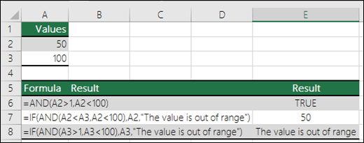
=AND(A2>1,A2<100) |
Displays TRUE if A2 is greater than 1 AND less than 100, otherwise it displays FALSE. |
|
=IF(AND(A2<A3,A2<100),A2,»The value is out of range») |
Displays the value in cell A2 if it’s less than A3 AND less than 100, otherwise it displays the message «The value is out of range». |
|
=IF(AND(A3>1,A3<100),A3,»The value is out of range») |
Displays the value in cell A3 if it is greater than 1 AND less than 100, otherwise it displays a message. You can substitute any message of your choice. |
Bonus Calculation
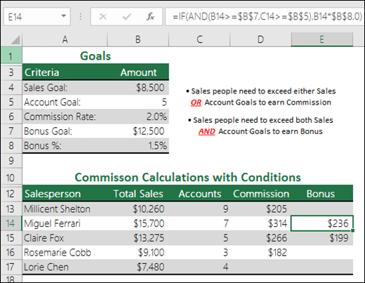
Here is a fairly common scenario where we need to calculate if sales people qualify for a bonus using IF and AND.
-
=IF(AND(B14>=$B$7,C14>=$B$5),B14*$B$8,0) – IF Total Sales are greater than or equal (>=) to the Sales Goal, AND Accounts are greater than or equal to (>=) the Account Goal, then multiply Total Sales by the Bonus %, otherwise return 0.
Need more help?
You can always ask an expert in the Excel Tech Community or get support in the Answers community.
Related Topics
Video: Advanced IF functions
Learn how to use nested functions in a formula
IF function
OR function
NOT function
Overview of formulas in Excel
How to avoid broken formulas
Detect errors in formulas
Keyboard shortcuts in Excel
Logical functions (reference)
Excel functions (alphabetical)
Excel functions (by category)
Need more help?
Want more options?
Explore subscription benefits, browse training courses, learn how to secure your device, and more.
Communities help you ask and answer questions, give feedback, and hear from experts with rich knowledge.
Purpose
Test multiple conditions with AND
Return value
TRUE if all arguments evaluate TRUE; FALSE if not
Usage notes
The AND function is used to check more than one logical condition at the same time, up to 255 conditions, supplied as arguments. Each argument (logical1, logical2, etc.) must be an expression that returns TRUE or FALSE or a value that can be evaluated as TRUE or FALSE. The arguments provided to the AND function can be constants, cell references, arrays, or logical expressions.
The purpose of the AND function is to evaluate more than one logical test at the same time and return TRUE only if all results are TRUE. For example, if A1 contains the number 50, then:
=AND(A1>0,A1>10,A1<100) // returns TRUE
=AND(A1>0,A1>10,A1<30) // returns FALSE
The AND function will evaluate all values supplied and return TRUE only if all values evaluate to TRUE. If any value evaluates to FALSE, the AND function will return FALSE. Note: Excel will evaluate any number except zero (0) as TRUE.
Both the AND function and the OR function will aggregate results to a single value. This means they can’t be used in array operations that need to deliver an array of results. To work around this limitation, you can use Boolean logic. For more information, see: Array formulas with AND and OR logic.
Examples
To test if the value in A1 is greater than 0 and less than 5, you can use AND like this:
=AND(A1>0,A1<5)
You can embed the AND function inside the IF function. Using the above example, you can supply AND as the logical_test for the IF function like so:
=IF(AND(A1>0,A1<5), "Approved", "Denied")
This formula will return «Approved» only if the value in A1 is greater than 0 and less than 5.
You can combine the AND function with the OR function. The formula below returns TRUE when A1 > 100 and B1 is «complete» or «pending»:
=AND(A1>100,OR(B1="complete",B1="pending"))
See below for many more examples of how the AND function can be used.
Notes
- The AND function is not case-sensitive.
- The AND function does not support wildcards.
- Text values or empty cells supplied as arguments are ignored.
- The AND function will return #VALUE if no logical values are found or created during evaluation.
The AND Function in excel is a logical function that tests multiple conditions and returns “true” or “false” depending on whether they are met or not. The formula of AND function is “=AND(logical1,[logical2]…),” where “logical1” is the first condition to evaluate.
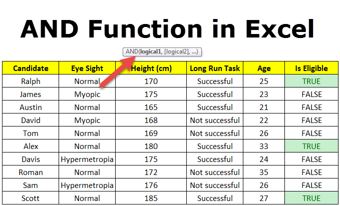
Table of contents
- AND Function in Excel
- Syntax of the AND Function
- The Characteristics of AND Function
- The Output of AND Function
- How to Use AND Function in Excel?
- Example #1–AND Function
- Example #2–AND Function With Nested IF Function
- Example #3–AND Function With Nested IF Function
- Nesting of AND Function in Excel
- Example #4–Nested AND Function
- Limitations of AND Function
- Frequently Asked Questions
- Recommended Articles
Syntax of the AND Function
The syntax is stated as follows:
The function accepts the following arguments:
- Logical 1: This is the first condition or logical value to evaluate.
- Logical 2: This is the second condition or logical value to evaluate.
The “logical 1” is a mandatory argument and “logical 2” is an optional argument.
The Characteristics of AND Function
- It returns “true” if all conditions or logical values evaluate to true.
- It returns “false” if any of the conditions or logical values evaluates to false.
- It can have more logical values depending on the situation and the requirement.
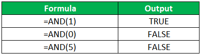
- It treats the value zero as “false” and all non-zero values as “true” while evaluating numbers.
- It ignores empty cells provided as an argument.
- It is often used in combination with other Excel functionsExcel functions help the users to save time and maintain extensive worksheets. There are 100+ excel functions categorized as financial, logical, text, date and time, Lookup & Reference, Math, Statistical and Information functions.read more like IF, OR, and so on.
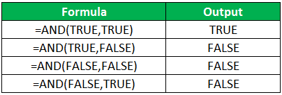
The Output of AND Function
The output in different situations is given as follows:
The output while evaluating numbers is given as follows:
How to Use AND Function in Excel?
It is easy to use the AND function. Let us understand its working with the help of a few examples.
You can download this AND Function Excel Template here – AND Function Excel Template
Example #1–AND Function
There are three levels and ten players in a game. To be a winner, a player has to clear all three levels. The player loses if he/she fails in any of the three levels.
The performance of the players in different levels is given in the following table. We are required to determine the winner.
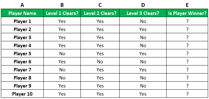
We apply AND formula in column E.
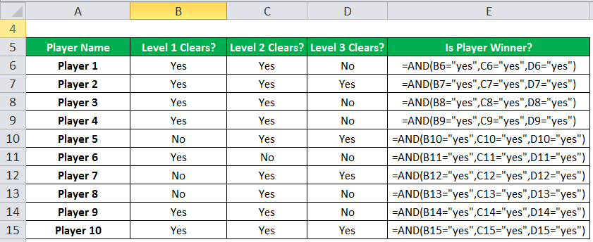
The output of the formula appears in column E.
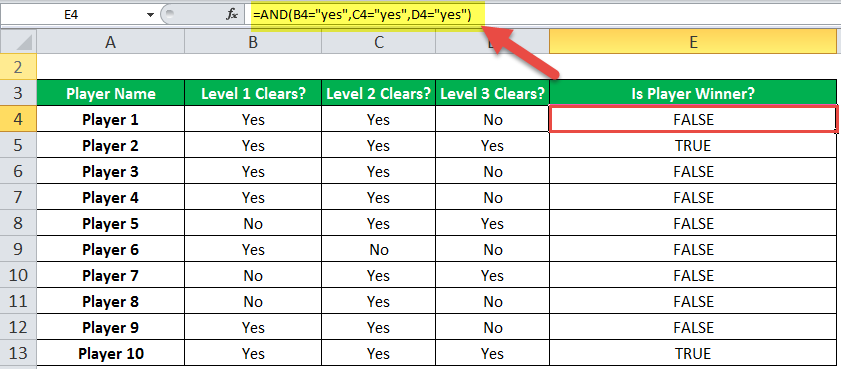
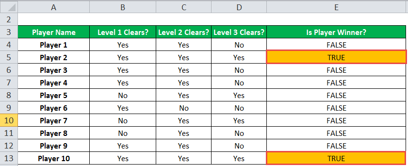
Player 2 and player 10 have cleared all the levels. Since all the logical conditions for these two players are met, the AND function gives the output “true.”
The rest of the players were unable to clear all three levels. If any of the levels is not cleared, the AND function returns “false.”
Example #2–AND Function With Nested IF Function
Let us consider the following example.
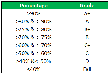
We have the marks (in percentage) of ten students in a school. We have to determine the grade obtained by each student according to the criteria given.
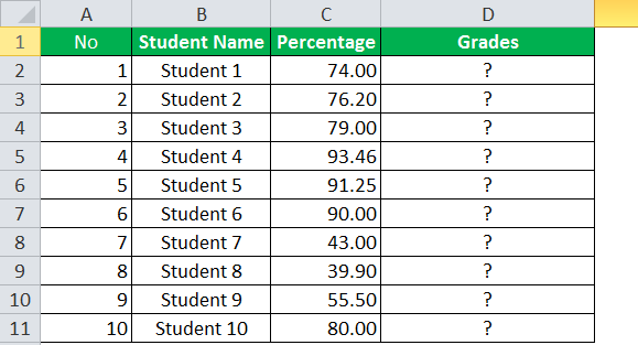
A student obtains “A+” if he/she scores more than 90%. If the percentage is greater than or equal to 80% but less than or equal to 90%, grade “A” is given.
If the percentage is less than 40%, the student fails. Likewise, the grades for the different percentages are given in the following table.
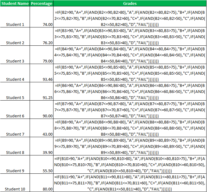
We apply the following formula.
“=IF(B2>90,”A+”,IF(AND(B2<=90,B2>80),”A”,IF(AND(B2<=80,B2>75),”B+”,IF(AND(B2<=75,B2>70),”B”,IF(AND(B2<=70,B2>60),”C+”,IF(AND(B2<=60,B2>50),”C”,IF(AND(B2<=50,B2>40),”D”,”FAIL”)))))))”
We use the nested IF functionIn Excel, nested if function means using another logical or conditional function with the if function to test multiple conditions. For example, if there are two conditions to be tested, we can use the logical functions AND or OR depending on the situation, or we can use the other conditional functions to test even more ifs inside a single if.read more with multiple AND functions to compute the grades. The latter allows testing two conditions together.
The syntax of the IF function is stated as follows:
“=IF(logical_test,[value_if_true],[value_if_false])”
The IF function returns “true” if the condition is met, else returns “false.”
The first logical test is “B2>90.” If this condition is “true,” grade “A+” is assigned. If this condition is “false,” the IF function evaluates the next condition.
The next logical testA logical test in Excel results in an analytical output, either true or false. The equals to operator, “=,” is the most commonly used logical test.read more is “B2<=90, B2>80.” If this condition is “true,” grade “A” is assigned. If this condition is “false,” the next statement is evaluated. Likewise, the IF function tests every condition given in the formula.
The last logical test is “B2<=50, B2>40.” If this condition is “true,” grade “D” is assigned, else the student fails.
We apply the formula to all categories of students, as shown in the following image.
The output of the formula is shown in the succeeding image.
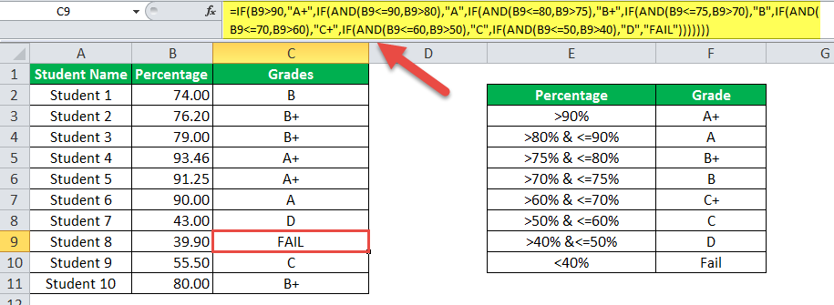
Example #3–AND Function With Nested IF Function
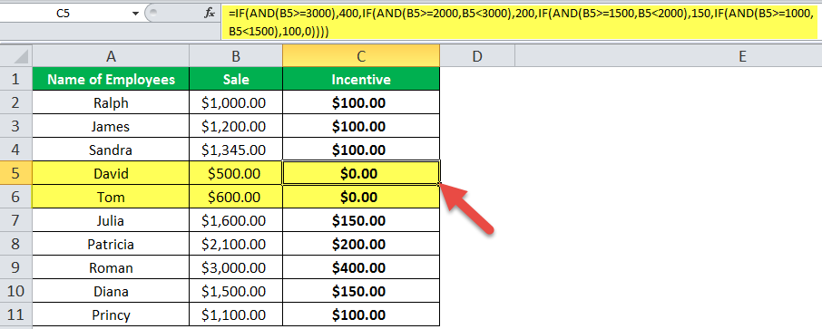
The name of employees and the sales revenueSales revenue refers to the income generated by any business entity by selling its goods or providing its services during the normal course of its operations. It is reported annually, quarterly or monthly as the case may be in the business entity’s income statement/profit & loss account.read more generated by them for an organization are shown in the succeeding image. Every employee is given a monetary incentive depending on the total sales made by him/her.
We have to calculate the incentives of all the employees based on their performance.
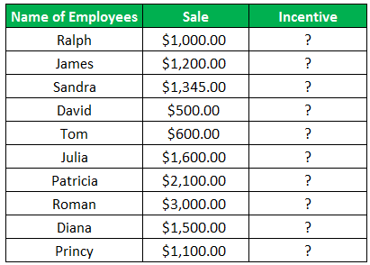
The incentive criteria followed by the organization is given in the succeeding table.
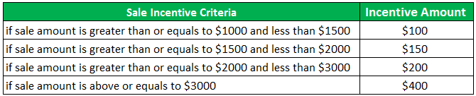
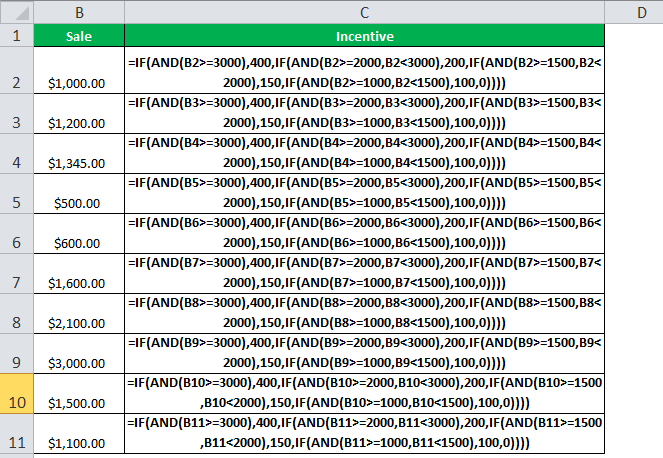
We apply the following formula.
“=IF(AND(B2>=3000),400,IF(AND(B2>=2000,B2<3000),200,IF(AND(B2>=1500,B2<2000),150,IF(AND(B2>=1000,B2<1500),100,0))))”
We use multiple IFs In Excel, multiple IF conditions are IF statements that are contained within another IF statement. They are used to test multiple conditions at the same time and return distinct values. Additional IF statements can be included in the ‘value if true’ and ‘value if false’ arguments of a standard IF formula.read moreand multiple AND functions to calculate the incentives received by all the employees, as shown in the following table.
Roman generates sales revenue of $3000. So, he receives an incentive amount of $400.
The revenue generated by David and Tom is $500 and $600, respectively. To be eligible for an incentive, minimum sales of $1000 is required. Hence, they do not get any incentive.
Nesting of AND Function in Excel
A nested function refers to using a function inside another Excel function. In Excel, the nesting of functions up to 64 levels is allowed.
Example #4–Nested AND Function
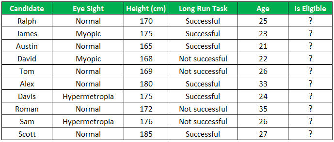
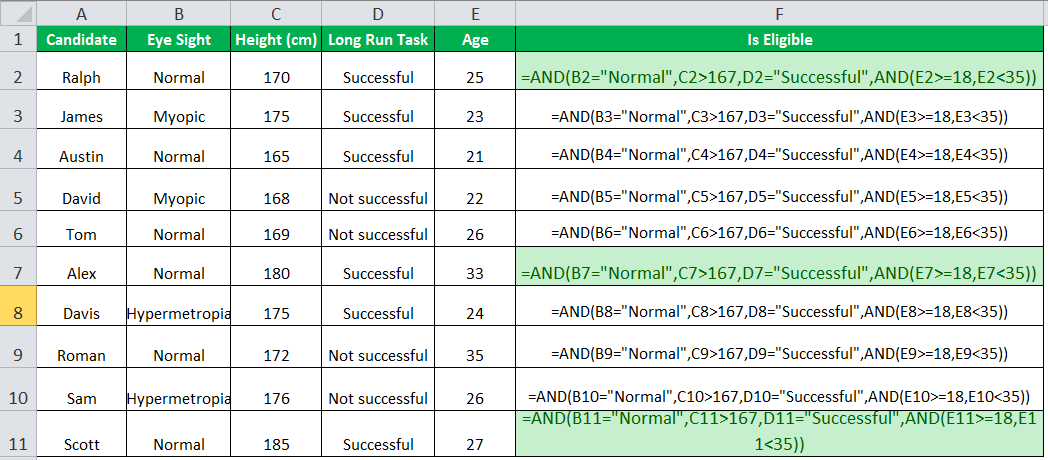
We have a list of candidates who wish to join the Army subject to certain conditions. The eligibility criteria are stated as follows:
- The age should be greater than or equal to 18, but less than 35 years.
- The height should be greater than 167 cm.
- The eyesight should be normal.
- The candidate must have completed the long-run task.
We need to find out the candidates who are eligible for joining the Army.
To evaluate the candidates on the given parameters, we use the nested AND function.
We apply the following formula.
“=AND(B2=”Normal”,C2>167,D2=”Successful”,AND(E2>=18,E2<35))”
We evaluate multiple logical conditions simultaneously. We also check whether the age is within the prescribed limit or not. So, we use the AND function inside another AND function.
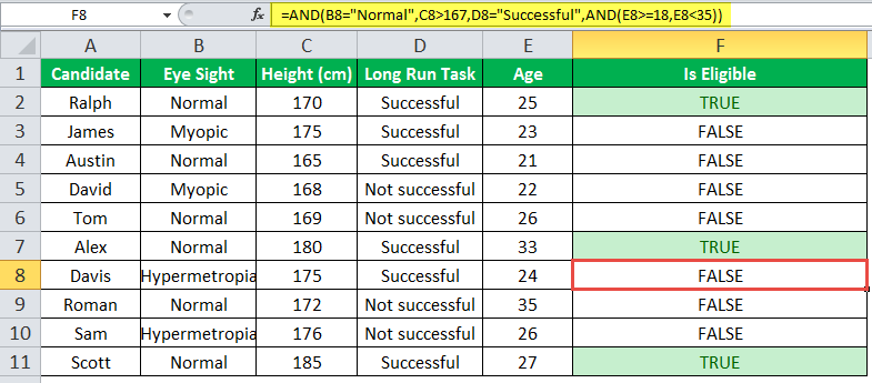
The output of the formula is shown in the succeeding image.
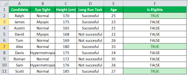
The candidates Ralph, Alex, and Scott pass the selection criteria. Hence, their eligibility output (in column F) is “true.” The remaining candidates are not eligible for joining the Army.
Limitations of AND Function
The limitations are listed as follows:
- With Excel 2007 onwards, the AND function can test up to 255 arguments given that the length of the formula does not exceed 8,162 characters.
- In Excel 2003 and previous versions, the AND function can test up to 30 arguments given that the length of the formula does not exceed 1,024 characters.
- The AND function returns “#VALUE! error#VALUE! Error in Excel represents that the reference cell the user has either entered an incorrect formula or used a wrong data type (mostly numerical data). Sometimes, it is difficult to identify the kind of mistake behind this error.read more” if logical conditions are passed as text or if none of the arguments evaluates to a logical value.
- The AND function returns “#VALUE! error” if all the arguments provided are empty cells.
The following two images show the output of the AND function when an empty cell and a text string is provided as an argument.

Frequently Asked Questions
#1 – When should the AND function of Excel be used
#2 – How is the AND function used with the OR function in Excel?
The OR function helps compare two values or statements. The AND function is combined with the OR function by the following formulas:
“=AND(OR(Condition1,Condition2),Condition3)”
“=AND(OR(Condition1,Condition2),OR(Condition3,Condition4)”
“=OR(AND(Condition1,Condition2),Condition3)”
“=OR(AND(Condition1,Condition2),AND(Condition3,Condition4))”
#3 – What is the difference between AND, IF, and OR functions in Excel?
The difference between the three functions is stated as follows:
– The AND function helps evaluate multiple conditions at the same time. It returns “true” when all conditions are true; otherwise, it returns “false.”
– The IF function helps compare the value with the result expected by the user. It returns specific values for the “true” and “false” outcomes.
– The OR function helps compare two values or two statements. It returns “true” when at least one of the specified conditions is met. It returns “false” if all the logical values evaluate to false.
- The AND function tests multiple conditions and returns “true” or “false” depending upon whether they are met or not.
- The AND function returns “true” if all conditions evaluate to true and returns “false” if any of the conditions evaluates to false.
- The AND function treats the value zero as “false.”
- The AND function can test up to 255 arguments in the latest versions of Excel.
- The AND function returns “#VALUE! error” if logical conditions are passed as a text.
- The formula of the IF function is “=IF(logical_test,[value_if_true],[value_if_false]).”
Recommended Articles
This has been a guide to AND Function in Excel. Here we discuss how to use AND Formula in Excel along with examples and downloadable excel templates. You may also look at these useful functions in Excel –
- Excel Pivot Table Add ColumnThe pivot table add column helps to add a new column in a pivot table.read more
- Excel Convert FunctionAs the word itself, the Excel CONVERT function defines that it can convert the numbers from one measurement system to another measurement system.read more
- VBA Boolean Data TypeBoolean is an inbuilt data type in VBA used for logical references or logical variables. The value this data type holds is either TRUE or FALSE and is used for logical comparison. The declaration of this data type is similar to all the other data types.read more
- IF AND Formula in ExcelThe IF AND excel formula is the combination of two different logical functions often nested together that enables the user to evaluate multiple conditions using AND functions. Based on the output of the AND function, the IF function returns either the “true” or “false” value, respectively.
read more
На чтение 2 мин
Функция AND (И) в Excel используется для сравнения нескольких условий.
Содержание
- Что возвращает функция
- Синтаксис
- Аргументы функции
- Дополнительная информация
- Примеры использования функции AND (И, ИЛИ) в Excel
Что возвращает функция
Возвращает TRUE если значение или условие, при сравнении, соответствует критериям заданным в функции, или FALSE, в случае, если условие не соответствует критериям.
Синтаксис
=AND(logical1, [logical2],…) — английская версия
=И(логическое_значение1;[логическое_значение2];…) — русская версия
Аргументы функции
- logical1 (логическое_значение1) — первое условие, которое вы хотите оценить с помощью функции;
- [logical2] ([логическое_значение2]) (не обязательно) — второе условие, которое вы хотите оценить с помощью функции.
Дополнительная информация
- Функция может быть использована совместно с другими формулами;
- Например, с помощью функции IF (ЕСЛИ) вы можете проверить условие, а затем указать значение, когда оно TRUE, и значение, когда оно равно FALSE. Использование функции AND (И) вместе с функцией IF (ЕСЛИ) позволяет тестировать несколько условий за один раз;
Например, если вы хотите проверить значение в ячейке A1 на предмет того, больше оно чем «0» или меньше чем «100», то вы можете использовать следующую формулу:
=IF(AND(A1>0,A1<100),”Approve”,”Reject”) — английская версия
Больше лайфхаков в нашем Telegram Подписаться
=ЕСЛИ(И(A1>0;A1<100);»Одобрить»;»Против») — русская версия
- Аргументы функции должны быть логически вычислимы по принципу (TRUE/FALSE);
- Ячейки с пустыми или текстовыми значениями игнорируются функцией;
- Если в качестве аргументов функции не указаны логически вычислимые данные, то функция выдаст ошибку #VALUE!;
- Одновременно вы можете тестировать до 255 условий в рамках одного использования функции.
Примеры использования функции AND (И, ИЛИ) в Excel

This Excel tutorial explains how to use the Excel AND function with syntax and examples.
Description
The Microsoft Excel AND function returns TRUE if all conditions are TRUE. It returns FALSE if any of the conditions are FALSE.
The AND function is a built-in function in Excel that is categorized as a Logical Function. It can be used as a worksheet function (WS) in Excel. As a worksheet function, the AND function can be entered as part of a formula in a cell of a worksheet.
Please read our AND function (VBA) page if you are looking for the VBA version of the AND function as it has a very different syntax.
Syntax
The syntax for the AND function in Microsoft Excel is:
AND( condition1, [condition2], ... )
Parameters or Arguments
- condition1
- The first condition to test whether it is TRUE or FALSE.
- condition2, …
- Optional. Additional conditions to test whether they are TRUE or FALSE. There can be up to 30 conditions in total.
Returns
The AND function returns TRUE if all conditions are TRUE.
The AND function returns FALSE if any of the conditions are FALSE.
Example (as Worksheet Function)
Let’s look at some Excel AND function examples and explore how to use the AND function as a worksheet function in Microsoft Excel:
Based on the Excel spreadsheet above, the following AND examples would return:
=AND(A1>10, A1<40)
Result: TRUE

=AND(A1=30, A2="www.checkyourmath.com")
Result: FALSE

=AND(A1>=5, A1<=30, A2="www.techonthenet.com")
Result: TRUE
Frequently Asked Questions
Question: I need to translate some Quattro Pro functions to Excel. The #AND# function in Qpro can be placed in the middle of a nest and return a number. For example, @if(…….A1>B1#and#A1<B3,7,0)
What this says is, after some other function, if A1 is greater than B1 and A1 is less than B3, return 7 otherwise 0. How do I get Excel to do this?
Answer: This can be done in Excel by combining the AND function with the IF function like this:
=IF(AND(A1>B1,A1<B3)=TRUE,7,0)
Question: In Microsoft Excel, I’m trying to use the If function to return 25 if cell A1 > 100 and cell B1 < 200. Otherwise, it should return 0.
Answer: You can use the AND function to perform an AND condition in the If function as follows:
=IF(AND(A1>100,B1<200),25,0)
In this example, the formula will return 25 if cell A1 is greater than 100 and cell B1 is less than 200. Otherwise, it will return 0.
Question: In Microsoft Excel, I want to write a formula for the following logic:
If R1 AND R2<0.3 AND R3<0.42 THEN «OK» OTHERWISE «NOT OK»
Answer: You can write an IF statement that uses the AND function as follows:
=IF(AND(R1<0.3,R2<0.3,R3<0.42),"OK","NOT OK")
Question: I have been looking at your Excel IF, AND and OR sections and found this very helpful, however I cannot find the right way to write a formula to express if C2 is either 1,2,3,4,5,6,7,8,9 and F2 is F and F3 is either D,F,B,L,R,C then give a value of 1 if not then 0. I have tried many formulas but just can’t get it right, can you help please?
Answer: You can write an IF statement that uses the AND function and the OR function as follows:
=IF(AND(C2>=1,C2<=9, F2="F",OR(F3="D",F3="F",F3="B",F3="L",F3="R",F3="C")),1,0)
Question:In Excel, I am trying to create a formula that will show the following:
If column B = Ross and column C = 8 then in cell AB of that row I want it to show 2013, If column B = Block and column C = 9 then in cell AB of that row I want it to show 2012.
Answer:You can create your Excel formula using nested IF functions with the AND function.
=IF(AND(B1="Ross",C1=8),2013,IF(AND(B1="Block",C1=9),2012,""))
This formula will return 2013 as a numeric value if B1 is «Ross» and C1 is 8, or 2012 as a numeric value if B1 is «Block» and C1 is 9. Otherwise, it will return blank, as denoted by «».
AND Function in Excel (Table of Contents)
- AND Function in Excel
- AND Formula in Excel
- How to use AND Function in Excel?
Excel AND Function
AND function is a logical function that is used when we need to carry to values or fields at the same time. AND Function returns the FALSE if any of the used logical values is FALSE. If we can to get the answer as TRUE, then all the logic used in AND function should be correct. Also, AND function works best when used with a combination of other conditional functions such as If, CountIf.
It is the most commonly used logical function alone or in combination with other operators like:
- “IF”
- “OR”
- “NOT”
- < (less than)
- > (greater than)
- = (equal to)
- <= (less than or equal to)
- >= (greater than or equal to)
- <> (not equal to)
It is most commonly used in conditional formatting.
AND function in Excel is used to test multiple conditions; up to 255 logical conditions can be used at the same time (Note: In Excel 2003 version, the function can only handle up to 30 arguments). AND function can operate on text, numbers, or cell references. AND function needs at least two arguments to return a value. A comma separates arguments; In the end, it provides either a ‘true’ or ‘false’ output based on the arguments inside the AND function.
AND Formula in Excel:
Below is the AND Formula in Excel.
logical1: logical value to evaluate, it’s a first condition to evaluate
logical2: logical value to evaluate, it’s a second condition to evaluate
How to Use the AND Function in Excel?
This AND function in excel is very simple easy to use. Let us now see how to use AND function in Excel with the help of some examples.
You can download this AND function in Excel Template here – AND function in Excel Template
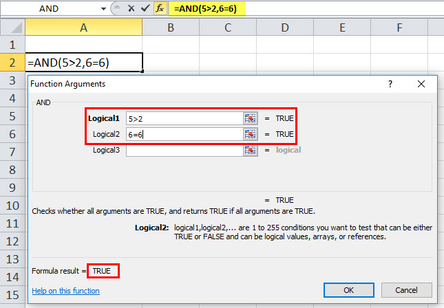
Example #1
If we enter =AND (5>2, 6=6) in an excel cell, the answer or formula result would be TRUE. It’s true because 5 is greater than 2 and 6 does equal 6.
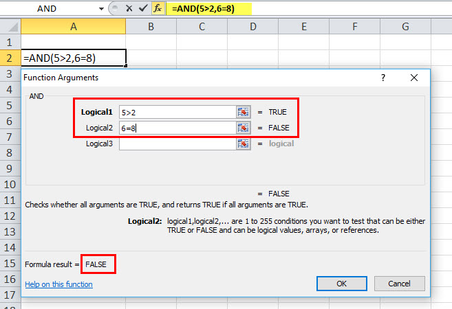
Example #2
If we enter =AND (5>2, 6=8) in an excel cell, the answer or formula result would be FALSE. It’s false because 5 is greater than 2, but 6 is not greater than 8
NOTE:
- In AND function formula, each term inside the parentheses is separated by a comma like other functions in excel.
- If an array or reference argument contains text or empty cells, those values are ignored.
- Suppose the specified range contains no logical values AND returns the #VALUE! error value.
Example #3
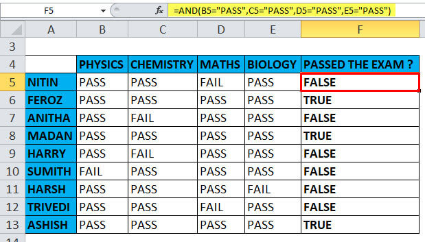
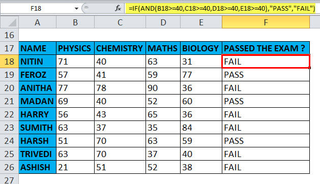
In this example, if a student passes all the subject, then he has passed the exam
=AND (B6=”PASS”, C6=”PASS”, D6=”PASS”, E6=”PASS”)
The text strings stored in column B, C, D & E, must be “PASS”. Each term inside the parentheses needs to be separated by a comma like other function in excel; here, it returns the value TRUE if all of the arguments evaluate TRUE. i.e. if students have passed all the subjects, it returns the value TRUE,
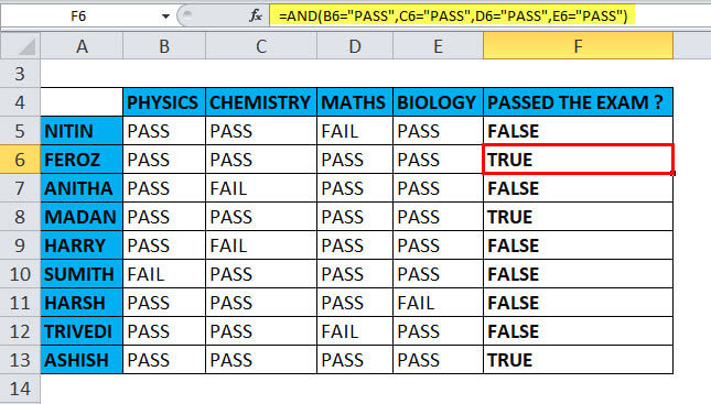
otherwise, even if the students have failed in any of the one subjects, it returns the value FALSE
Example #4
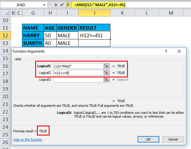
Using other operators (> (greater than) = (equal to) along with AND Function
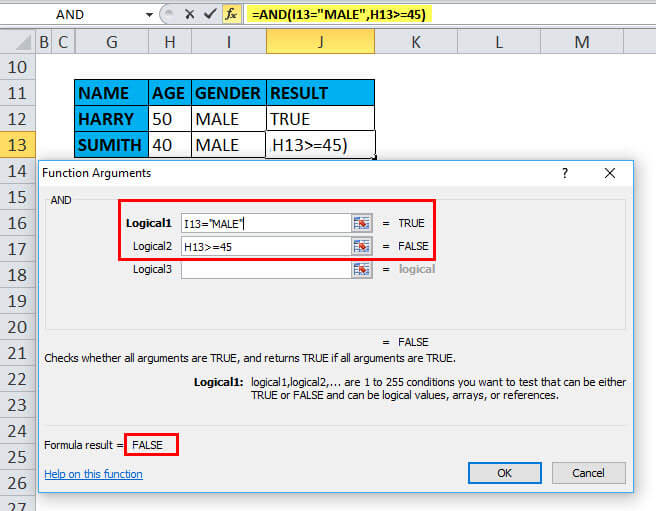
AND function returns TRUE if first logical condition, Gender parameter I12 = MALE, and the second logical condition, age parameter should be equal to or more than 45 years, i.e. H12>=45. else it returns FALSE. Herewith reference to HARRY, it returns the value TRUE,
In the case of other candidates, SUMITH, it returns the value FALSE.
Example #5
Using AND with “IF” Function with other operators
Suppose you have a table with the various subject score, need to find out the results of the exam whether they have passed the exam or not
The first score, stored in column B with the first subject, must be equal to or greater than 40. The second score, listed in column C with the second subject, must be equal to or greater than 40. Similarly, the third & fourth score, with third & fourth subject stored in column D & E, must be equal to or greater than 40. If all the above four conditions are met, a student passes the exam.
The easiest way to make a proper IF/AND formula is to initially write down the condition first and later add it in the logical test argument of your IF function:
Condition: AND(B18>=40, C18>=40, D18>=40, E18>=40)
IF/AND formula: =IF( AND(B18>=40, C18>=40, D18>=40, E18>=40), “PASS”, “FAIL”)
Example #6
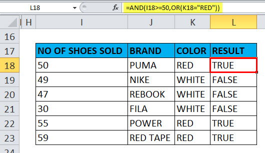
Using AND function with “OR” FUNCTION
Using IF and AND together is actually quite simple; in the below-mentioned example, irrespective of brand, in the table array, need to find out the sales of red color shoes which are more than 50 numbers by using AND function with “OR” function.
The first column contains the number of shoes sold; the second column contains the brand of shoes, the third column contains color of shoes, Here the condition is data in the I column should be equal to, or more than 50 & simultaneously the color of the shoes should be red. If both the above conditions are met, it returns the value “TRUE” otherwise “FALSE.”
Recommended Articles
This is a guide to AND Function in Excel. Here we discuss the AND Formula in Excel and how to use AND in Excel and practical examples and downloadable excel templates. You can also go through our other suggested articles –
- OR Excel Function
- VBA AND
- Logical Functions in Excel
- COS Function in Excel
Функция
И(
)
, английский вариант AND(),
проверяет на истинность условия и возвращает ИСТИНА если все условия истинны или ЛОЖЬ если хотя бы одно ложно.
Синтаксис функции
И(логическое_значение1; [логическое_значение2]; …)
логическое_значение
— любое значение или выражение, принимающее значения ИСТИНА или ЛОЖЬ.
Например,
=И(A1>100;A2>100)
Т.е. если в
обеих
ячейках
A1
и
A2
содержатся значения больше 100 (т.е. выражение
A1>100
— ИСТИНА
и
выражение
A2>100
— ИСТИНА), то формула вернет
ИСТИНА,
а если хотя бы в одной ячейке значение <=100, то формула вернет
ЛОЖЬ
.
Другими словами, формула
=И(ИСТИНА;ИСТИНА)
вернет ИСТИНА, а формулы
=И(ИСТИНА;ЛОЖЬ)
или
=И(ЛОЖЬ;ИСТИНА)
или
=И(ЛОЖЬ;ЛОЖЬ)
или
=И(ЛОЖЬ;ИСТИНА;ИСТИНА)
вернут ЛОЖЬ.
Функция воспринимает от 1 до 255 проверяемых условий. Понятно, что 1 значение использовать бессмысленно, для этого есть функция
ЕСЛИ()
. Чаще всего функцией
И()
на истинность проверяется 2-5 условий.
Совместное использование с функцией
ЕСЛИ()
Сама по себе функция
И()
имеет ограниченное использование, т.к. она может вернуть только значения ИСТИНА или ЛОЖЬ, чаще всего ее используют вместе с функцией
ЕСЛИ()
:
=ЕСЛИ(И(A1>100;A2>100);»Бюджет превышен»;»В рамках бюджета»)
Т.е. если в
обеих
ячейках
A1
и
A2
содержатся значения больше 100, то выводится
Бюджет превышен
, если хотя бы в одной ячейке значение <=100, то
В рамках бюджета
.
Сравнение с функцией
ИЛИ()
Функция
ИЛИ()
также может вернуть только значения ИСТИНА или ЛОЖЬ, но, в отличие от
И()
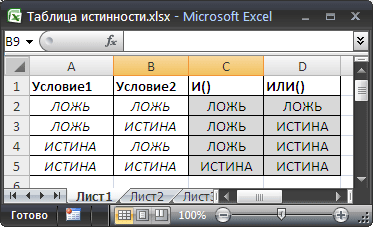
, она возвращает ЛОЖЬ, только если все ее условия ложны. Чтобы сравнить эти функции составим, так называемую таблицу истинности для
И()
и
ИЛИ()
.
Эквивалентность функции
И()
операции умножения *
В математических вычислениях EXCEL интерпретирует значение ЛОЖЬ как 0, а ИСТИНА как 1. В этом легко убедиться записав формулы
=ИСТИНА+0
и
=ЛОЖЬ+0
Следствием этого является возможность альтернативной записи формулы
=И(A1>100;A2>100)
в виде
=(A1>100)*(A2>100)
Значение второй формулы будет =1 (ИСТИНА), только если оба аргумента истинны, т.е. равны 1. Только произведение 2-х единиц даст 1 (ИСТИНА), что совпадает с определением функции
И()
.
Эквивалентность функции
И()
операции умножения * часто используется в формулах с Условием И, например, для того чтобы сложить только те значения, которые больше 5
И
меньше 10:
=СУММПРОИЗВ((A1:A10>5)*(A1:A10<10)*(A1:A10))
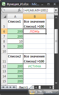
Проверка множества однотипных условий
Предположим, что необходимо проверить все значения в диапазоне
A6:A9
на превышение некоторого граничного значения, например 100. Можно, конечно записать формулу
=И(A6>100;A7>100;A8>100;A9>100)
но существует более компактная формула, правда которую нужно ввести как
формулу массива
(см.
файл примера
):
=И(A6:A9>100)
(для ввода формулы в ячейку вместо
ENTER
нужно нажать
CTRL+SHIFT+ENTER
)
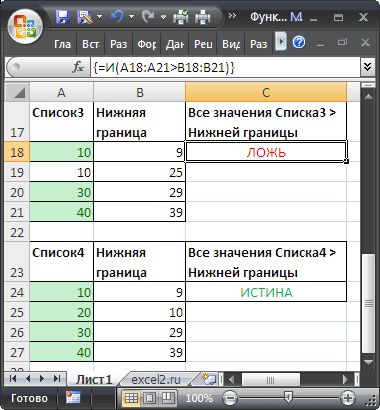
В случае, если границы для каждого проверяемого значения разные, то границы можно ввести в соседний столбец и организовать
попарное сравнение списков
с помощью
формулы массива
:
=И(A18:A21>B18:B21)
Вместо диапазона с границами можно также использовать
константу массива
:
=И(A18:A21>{9:25:29:39})
Determines if the given conditions in a test are TRUE
What is the AND Function?
The AND Function[1] is categorized under Excel Logical functions. It is used to determine if the given conditions in a test are TRUE. For example, we can use the function to test if a number in cell B1 is greater than 50 and less than 100.
As a financial analyst, the function is useful in testing multiple conditions, specifically, if multiple conditions are met to make sure they all are true. Also, it helps us avoid extra nested IFS, and the AND function can be combined with the OR function.
Formula
=AND(logical1, [logical2], …)
The AND function uses the following arguments:
- Logical1 (required argument) – This is the first condition or logical value to be evaluated.
- Logical2 (optional requirement) – This is the second condition or logical value to be evaluated.
Notes:
- We can set up to 255 conditions for the AND function.
- The function tests a number of supplied conditions and returns:
- TRUE if ALL of the conditions evaluate to TRUE; or
- FALSE otherwise (i.e., if ANY of the conditions evaluate to FALSE).
How to Use the AND Function in Excel?
To understand the uses of the AND function, let us consider a few examples:
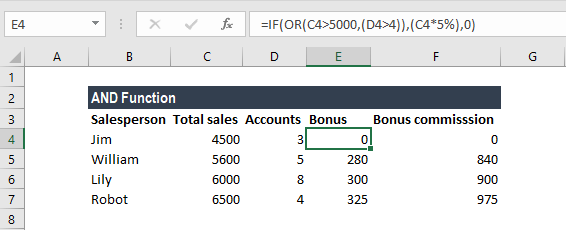
Example 1
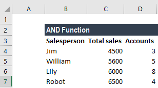
Suppose we wish to calculate the bonus for every salesperson in our company. To be eligible for a 5% bonus, the salesperson should have achieved sales higher than $5,000 in a year. Otherwise, they should have achieved an account goal of 4 accounts or higher. To earn a bonus of 15%, they should have achieved both conditions together.
We are given the data given below:
To calculate the bonus commission, we will use the AND function. The formula will be:
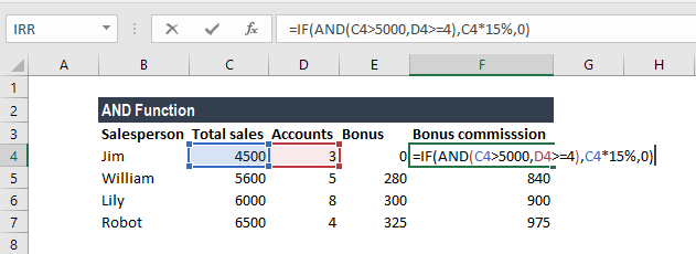
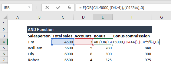
The formula for calculating the bonus does not require the AND function but we need to use the OR function. The formula to use will be:
The resulting table will be similar to the one below:
Example 2
Let’s see how we can use the AND function to test if a numeric value falls between two specific numbers. For this, we can use the AND function with two logical tests.
Suppose we are given the data below:
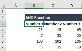
The formula to use is:
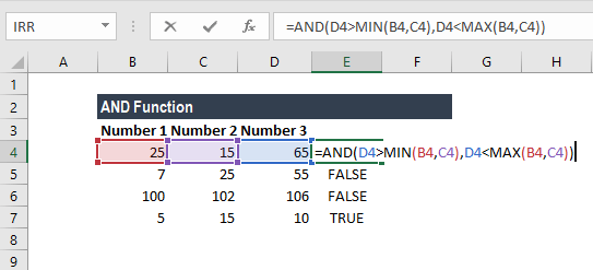
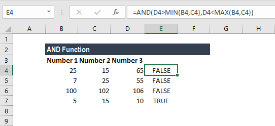
In the above formula, the value is compared to the smaller of the two numbers, determined by the MIN function. In the second expression, the value is compared to the larger of the two numbers, determined by the MAX function. The AND function will return TRUE only when the value is greater than the smaller number and less than the larger number.
We get the results below:
Things to Remember about the AND Function
- VALUE! error – Occurs when no logical values are found or created during the evaluation.
- Test values or empty cells provided as arguments are ignored by the AND function.
Click here to download the sample Excel file
Additional Resources
Thanks for reading CFI’s guide to important Excel functions! By taking the time to learn and master these functions, you’ll significantly speed up your financial analysis. To learn more, check out these additional CFI resources:
- Advanced Excel Course
- Advanced Excel Formulas You Must Know
- Excel Shortcuts for Windows and Mac
- Financial Modeling Program
- See all Excel resources
Article Sources
- AND Function