The IF function allows you to make a logical comparison between a value and what you expect by testing for a condition and returning a result if that condition is True or False.
-
=IF(Something is True, then do something, otherwise do something else)
But what if you need to test multiple conditions, where let’s say all conditions need to be True or False (AND), or only one condition needs to be True or False (OR), or if you want to check if a condition does NOT meet your criteria? All 3 functions can be used on their own, but it’s much more common to see them paired with IF functions.
Use the IF function along with AND, OR and NOT to perform multiple evaluations if conditions are True or False.
Syntax
-
IF(AND()) — IF(AND(logical1, [logical2], …), value_if_true, [value_if_false]))
-
IF(OR()) — IF(OR(logical1, [logical2], …), value_if_true, [value_if_false]))
-
IF(NOT()) — IF(NOT(logical1), value_if_true, [value_if_false]))
|
Argument name |
Description |
|
|
logical_test (required) |
The condition you want to test. |
|
|
value_if_true (required) |
The value that you want returned if the result of logical_test is TRUE. |
|
|
value_if_false (optional) |
The value that you want returned if the result of logical_test is FALSE. |
|
Here are overviews of how to structure AND, OR and NOT functions individually. When you combine each one of them with an IF statement, they read like this:
-
AND – =IF(AND(Something is True, Something else is True), Value if True, Value if False)
-
OR – =IF(OR(Something is True, Something else is True), Value if True, Value if False)
-
NOT – =IF(NOT(Something is True), Value if True, Value if False)
Examples
Following are examples of some common nested IF(AND()), IF(OR()) and IF(NOT()) statements. The AND and OR functions can support up to 255 individual conditions, but it’s not good practice to use more than a few because complex, nested formulas can get very difficult to build, test and maintain. The NOT function only takes one condition.
Here are the formulas spelled out according to their logic:
|
Formula |
Description |
|---|---|
|
=IF(AND(A2>0,B2<100),TRUE, FALSE) |
IF A2 (25) is greater than 0, AND B2 (75) is less than 100, then return TRUE, otherwise return FALSE. In this case both conditions are true, so TRUE is returned. |
|
=IF(AND(A3=»Red»,B3=»Green»),TRUE,FALSE) |
If A3 (“Blue”) = “Red”, AND B3 (“Green”) equals “Green” then return TRUE, otherwise return FALSE. In this case only the first condition is true, so FALSE is returned. |
|
=IF(OR(A4>0,B4<50),TRUE, FALSE) |
IF A4 (25) is greater than 0, OR B4 (75) is less than 50, then return TRUE, otherwise return FALSE. In this case, only the first condition is TRUE, but since OR only requires one argument to be true the formula returns TRUE. |
|
=IF(OR(A5=»Red»,B5=»Green»),TRUE,FALSE) |
IF A5 (“Blue”) equals “Red”, OR B5 (“Green”) equals “Green” then return TRUE, otherwise return FALSE. In this case, the second argument is True, so the formula returns TRUE. |
|
=IF(NOT(A6>50),TRUE,FALSE) |
IF A6 (25) is NOT greater than 50, then return TRUE, otherwise return FALSE. In this case 25 is not greater than 50, so the formula returns TRUE. |
|
=IF(NOT(A7=»Red»),TRUE,FALSE) |
IF A7 (“Blue”) is NOT equal to “Red”, then return TRUE, otherwise return FALSE. |
Note that all of the examples have a closing parenthesis after their respective conditions are entered. The remaining True/False arguments are then left as part of the outer IF statement. You can also substitute Text or Numeric values for the TRUE/FALSE values to be returned in the examples.
Here are some examples of using AND, OR and NOT to evaluate dates.
Here are the formulas spelled out according to their logic:
|
Formula |
Description |
|---|---|
|
=IF(A2>B2,TRUE,FALSE) |
IF A2 is greater than B2, return TRUE, otherwise return FALSE. 03/12/14 is greater than 01/01/14, so the formula returns TRUE. |
|
=IF(AND(A3>B2,A3<C2),TRUE,FALSE) |
IF A3 is greater than B2 AND A3 is less than C2, return TRUE, otherwise return FALSE. In this case both arguments are true, so the formula returns TRUE. |
|
=IF(OR(A4>B2,A4<B2+60),TRUE,FALSE) |
IF A4 is greater than B2 OR A4 is less than B2 + 60, return TRUE, otherwise return FALSE. In this case the first argument is true, but the second is false. Since OR only needs one of the arguments to be true, the formula returns TRUE. If you use the Evaluate Formula Wizard from the Formula tab you’ll see how Excel evaluates the formula. |
|
=IF(NOT(A5>B2),TRUE,FALSE) |
IF A5 is not greater than B2, then return TRUE, otherwise return FALSE. In this case, A5 is greater than B2, so the formula returns FALSE. |
Using AND, OR and NOT with Conditional Formatting
You can also use AND, OR and NOT to set Conditional Formatting criteria with the formula option. When you do this you can omit the IF function and use AND, OR and NOT on their own.
From the Home tab, click Conditional Formatting > New Rule. Next, select the “Use a formula to determine which cells to format” option, enter your formula and apply the format of your choice.
Using the earlier Dates example, here is what the formulas would be.
|
Formula |
Description |
|---|---|
|
=A2>B2 |
If A2 is greater than B2, format the cell, otherwise do nothing. |
|
=AND(A3>B2,A3<C2) |
If A3 is greater than B2 AND A3 is less than C2, format the cell, otherwise do nothing. |
|
=OR(A4>B2,A4<B2+60) |
If A4 is greater than B2 OR A4 is less than B2 plus 60 (days), then format the cell, otherwise do nothing. |
|
=NOT(A5>B2) |
If A5 is NOT greater than B2, format the cell, otherwise do nothing. In this case A5 is greater than B2, so the result will return FALSE. If you were to change the formula to =NOT(B2>A5) it would return TRUE and the cell would be formatted. |
Note: A common error is to enter your formula into Conditional Formatting without the equals sign (=). If you do this you’ll see that the Conditional Formatting dialog will add the equals sign and quotes to the formula — =»OR(A4>B2,A4<B2+60)», so you’ll need to remove the quotes before the formula will respond properly.
Need more help?

See also
You can always ask an expert in the Excel Tech Community or get support in the Answers community.
Learn how to use nested functions in a formula
IF function
AND function
OR function
NOT function
Overview of formulas in Excel
How to avoid broken formulas
Detect errors in formulas
Keyboard shortcuts in Excel
Logical functions (reference)
Excel functions (alphabetical)
Excel functions (by category)
Содержание
- AND function
- Example
- Examples
- Need more help?
- IF function
- Simple IF examples
- Common problems
- Need more help?
- Use AND and OR to test a combination of conditions
- Use AND and OR with IF
- Sample data
- Using IF with AND, OR and NOT functions
- Examples
- Using AND, OR and NOT with Conditional Formatting
- Need more help?
- See also
- Create conditional formulas
- What do you want to do?
- Create a conditional formula that results in a logical value (TRUE or FALSE)
- Example
- Create a conditional formula that results in another calculation or in values other than TRUE or FALSE
- Example
AND function
Use the AND function, one of the logical functions, to determine if all conditions in a test are TRUE.
Example
The AND function returns TRUE if all its arguments evaluate to TRUE, and returns FALSE if one or more arguments evaluate to FALSE.
One common use for the AND function is to expand the usefulness of other functions that perform logical tests. For example, the IF function performs a logical test and then returns one value if the test evaluates to TRUE and another value if the test evaluates to FALSE. By using the AND function as the logical_test argument of the IF function, you can test many different conditions instead of just one.
The AND function syntax has the following arguments:
Required. The first condition that you want to test that can evaluate to either TRUE or FALSE.
Optional. Additional conditions that you want to test that can evaluate to either TRUE or FALSE, up to a maximum of 255 conditions.
The arguments must evaluate to logical values, such as TRUE or FALSE, or the arguments must be arrays or references that contain logical values.
If an array or reference argument contains text or empty cells, those values are ignored.
If the specified range contains no logical values, the AND function returns the #VALUE! error.
Examples
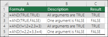
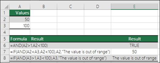
Here are some general examples of using AND by itself, and in conjunction with the IF function.
=AND(A2>1,A2 AND less than 100, otherwise it displays FALSE.
Displays the value in cell A2 if it’s less than A3 AND less than 100, otherwise it displays the message «The value is out of range».
=IF(AND(A3>1,A3 AND less than 100, otherwise it displays a message. You can substitute any message of your choice.
Here is a fairly common scenario where we need to calculate if sales people qualify for a bonus using IF and AND.
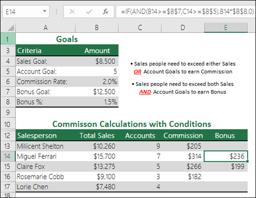
=IF(AND(B14>=$B$7,C14>=$B$5),B14*$B$8,0) – IF Total Sales are greater than or equal (>=) to the Sales Goal, AND Accounts are greater than or equal to (>=) the Account Goal, then multiply Total Sales by the Bonus %, otherwise return 0.
Need more help?
You can always ask an expert in the Excel Tech Community or get support in the Answers community.
Источник
IF function
The IF function is one of the most popular functions in Excel, and it allows you to make logical comparisons between a value and what you expect.
So an IF statement can have two results. The first result is if your comparison is True, the second if your comparison is False.
For example, =IF(C2=”Yes”,1,2) says IF(C2 = Yes, then return a 1, otherwise return a 2).
Use the IF function, one of the logical functions, to return one value if a condition is true and another value if it’s false.
IF(logical_test, value_if_true, [value_if_false])
The condition you want to test.
The value that you want returned if the result of logical_test is TRUE.
The value that you want returned if the result of logical_test is FALSE.
Simple IF examples
In the above example, cell D2 says: IF(C2 = Yes, then return a 1, otherwise return a 2)
In this example, the formula in cell D2 says: IF(C2 = 1, then return Yes, otherwise return No)As you see, the IF function can be used to evaluate both text and values. It can also be used to evaluate errors. You are not limited to only checking if one thing is equal to another and returning a single result, you can also use mathematical operators and perform additional calculations depending on your criteria. You can also nest multiple IF functions together in order to perform multiple comparisons.

=IF(C2>B2,”Over Budget”,”Within Budget”)
In the above example, the IF function in D2 is saying IF(C2 Is Greater Than B2, then return “Over Budget”, otherwise return “Within Budget”)

In the above illustration, instead of returning a text result, we are going to return a mathematical calculation. So the formula in E2 is saying IF(Actual is Greater than Budgeted, then Subtract the Budgeted amount from the Actual amount, otherwise return nothing).
In this example, the formula in F7 is saying IF(E7 = “Yes”, then calculate the Total Amount in F5 * 8.25%, otherwise no Sales Tax is due so return 0)
Note: If you are going to use text in formulas, you need to wrap the text in quotes (e.g. “Text”). The only exception to that is using TRUE or FALSE, which Excel automatically understands.
Common problems
What went wrong
There was no argument for either value_if_true or value_if_False arguments. To see the right value returned, add argument text to the two arguments, or add TRUE or FALSE to the argument.
This usually means that the formula is misspelled.
Need more help?
You can always ask an expert in the Excel Tech Community or get support in the Answers community.
Источник
Use AND and OR to test a combination of conditions
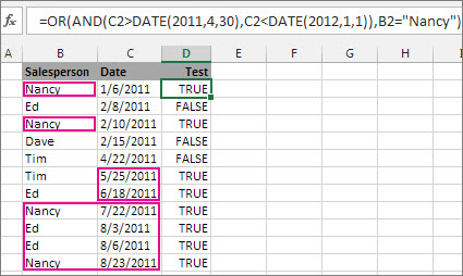
When you need to find data that meets more than one condition, such as units sold between April and January, or units sold by Nancy, you can use the AND and OR functions together. Here’s an example:
This formula nests the AND function inside the OR function to search for units sold between April 1, 2011 and January 1, 2012, or any units sold by Nancy. You can see it returns True for units sold by Nancy, and also for units sold by Tim and Ed during the dates specified in the formula.
Here’s the formula in a form you can copy and paste. If you want to play with it in a sample workbook, see the end of this article.
Use AND and OR with IF
You can also use AND and OR with the IF function.
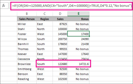
In this example, people don’t earn bonuses until they sell at least $125,000 worth of goods, unless they work in the southern region where the market is smaller. In that case, they qualify for a bonus after $100,000 in sales.
Let’s look a bit deeper. The IF function requires three pieces of data (arguments) to run properly. The first is a logical test, the second is the value you want to see if the test returns True, and the third is the value you want to see if the test returns False. In this example, the OR function and everything nested in it provides the logical test. You can read it as: Look for values greater than or equal to 125,000, unless the value in column C is «South», then look for a value greater than 100,000, and every time both conditions are true, multiply the value by 0.12, the commission amount. Otherwise, display the words «No bonus.»
Sample data
If you want to work with the examples in this article, copy the following table into cell A1 in your own spreadsheet. Be sure to select the whole table, including the heading row.
Источник
Using IF with AND, OR and NOT functions
The IF function allows you to make a logical comparison between a value and what you expect by testing for a condition and returning a result if that condition is True or False.
=IF(Something is True, then do something, otherwise do something else)
But what if you need to test multiple conditions, where let’s say all conditions need to be True or False ( AND), or only one condition needs to be True or False ( OR), or if you want to check if a condition does NOT meet your criteria? All 3 functions can be used on their own, but it’s much more common to see them paired with IF functions.
Use the IF function along with AND, OR and NOT to perform multiple evaluations if conditions are True or False.
IF(AND()) — IF(AND(logical1, [logical2], . ), value_if_true, [value_if_false]))
IF(OR()) — IF(OR(logical1, [logical2], . ), value_if_true, [value_if_false]))
IF(NOT()) — IF(NOT(logical1), value_if_true, [value_if_false]))
The condition you want to test.
The value that you want returned if the result of logical_test is TRUE.
The value that you want returned if the result of logical_test is FALSE.
Here are overviews of how to structure AND, OR and NOT functions individually. When you combine each one of them with an IF statement, they read like this:
AND – =IF(AND(Something is True, Something else is True), Value if True, Value if False)
OR – =IF(OR(Something is True, Something else is True), Value if True, Value if False)
NOT – =IF(NOT(Something is True), Value if True, Value if False)
Examples
Following are examples of some common nested IF(AND()), IF(OR()) and IF(NOT()) statements. The AND and OR functions can support up to 255 individual conditions, but it’s not good practice to use more than a few because complex, nested formulas can get very difficult to build, test and maintain. The NOT function only takes one condition.
Here are the formulas spelled out according to their logic:
=IF(AND(A2>0,B2 0,B4 50),TRUE,FALSE)
IF A6 (25) is NOT greater than 50, then return TRUE, otherwise return FALSE. In this case 25 is not greater than 50, so the formula returns TRUE.
IF A7 (“Blue”) is NOT equal to “Red”, then return TRUE, otherwise return FALSE.
Note that all of the examples have a closing parenthesis after their respective conditions are entered. The remaining True/False arguments are then left as part of the outer IF statement. You can also substitute Text or Numeric values for the TRUE/FALSE values to be returned in the examples.
Here are some examples of using AND, OR and NOT to evaluate dates.
Here are the formulas spelled out according to their logic:
IF A2 is greater than B2, return TRUE, otherwise return FALSE. 03/12/14 is greater than 01/01/14, so the formula returns TRUE.
=IF(AND(A3>B2,A3 B2,A4 B2),TRUE,FALSE)
IF A5 is not greater than B2, then return TRUE, otherwise return FALSE. In this case, A5 is greater than B2, so the formula returns FALSE.
Using AND, OR and NOT with Conditional Formatting
You can also use AND, OR and NOT to set Conditional Formatting criteria with the formula option. When you do this you can omit the IF function and use AND, OR and NOT on their own.
From the Home tab, click Conditional Formatting > New Rule. Next, select the “ Use a formula to determine which cells to format” option, enter your formula and apply the format of your choice.

Using the earlier Dates example, here is what the formulas would be.
If A2 is greater than B2, format the cell, otherwise do nothing.
=AND(A3>B2,A3 B2,A4 B2)
If A5 is NOT greater than B2, format the cell, otherwise do nothing. In this case A5 is greater than B2, so the result will return FALSE. If you were to change the formula to =NOT(B2>A5) it would return TRUE and the cell would be formatted.
Note: A common error is to enter your formula into Conditional Formatting without the equals sign (=). If you do this you’ll see that the Conditional Formatting dialog will add the equals sign and quotes to the formula — =»OR(A4>B2,A4
Need more help?

See also
You can always ask an expert in the Excel Tech Community or get support in the Answers community.
Источник
Create conditional formulas
Testing whether conditions are true or false and making logical comparisons between expressions are common to many tasks. You can use the AND, OR, NOT, and IF functions to create conditional formulas.
For example, the IF function uses the following arguments.
Formula that uses the IF function


For more information about how to create formulas, see Create or delete a formula.
What do you want to do?
Create a conditional formula that results in a logical value (TRUE or FALSE)
To do this task, use the AND, OR, and NOT functions and operators as shown in the following example.
Example
The example may be easier to understand if you copy it to a blank worksheet.
How do I copy an example?
Select the example in this article.
Selecting an example from Help
In Excel, create a blank workbook or worksheet.
In the worksheet, select cell A1, and press CTRL+V.
Important: For the example to work properly, you must paste it into cell A1 of the worksheet.
To switch between viewing the results and viewing the formulas that return the results, press CTRL+` (grave accent), or on the Formulas tab, in the Formula Auditing group, click the Show Formulas button.
After you copy the example to a blank worksheet, you can adapt it to suit your needs.
Determines if the value in cell A2 is greater than the value in A3 and also if the value in A2 is less than the value in A4. (FALSE)
Determines if the value in cell A2 is greater than the value in A3 or if the value in A2 is less than the value in A4. (TRUE)
Determines if the sum of the values in cells A2 and A3 is not equal to 24. (FALSE)
Determines if the value in cell A5 is not equal to «Sprockets.» (FALSE)
Determines if the value in cell A5 is not equal to «Sprockets» or if the value in A6 is equal to «Widgets.» (TRUE)
For more information about how to use these functions, see AND function, OR function, and NOT function.
Create a conditional formula that results in another calculation or in values other than TRUE or FALSE
To do this task, use the IF, AND, and OR functions and operators as shown in the following example.
Example
The example may be easier to understand if you copy it to a blank worksheet.
How do I copy an example?
Select the example in this article.
Important: Do not select the row or column headers.
Selecting an example from Help
In Excel, create a blank workbook or worksheet.
In the worksheet, select cell A1, and press CTRL+V.
Important: For the example to work properly, you must paste it into cell A1 of the worksheet.
To switch between viewing the results and viewing the formulas that return the results, press CTRL+` (grave accent), or on the Formulas tab, in the Formula Auditing group, click the Show Formulas button.
After you copy the example to a blank worksheet, you can adapt it to suit your needs.
=IF(A2=15, «OK», «Not OK»)
If the value in cell A2 equals 15, return «OK.» Otherwise, return «Not OK.» (OK)
=IF(A2<>15, «OK», «Not OK»)
If the value in cell A2 is not equal to 15, return «OK.» Otherwise, return «Not OK.» (Not OK)
=IF(NOT(A2 «SPROCKETS», «OK», «Not OK»)
If the value in cell A5 is not equal to «SPROCKETS», return «OK.» Otherwise, return «Not OK.» (Not OK)
If the value in cell A2 is greater than the value in A3 and the value in A2 is also less than the value in A4, return «OK.» Otherwise, return «Not OK.» (Not OK)
=IF(AND(A2<>A3, A2<>A4), «OK», «Not OK»)
If the value in cell A2 is not equal to A3 and the value in A2 is also not equal to the value in A4, return «OK.» Otherwise, return «Not OK.» (OK)
If the value in cell A2 is greater than the value in A3 or the value in A2 is less than the value in A4, return «OK.» Otherwise, return «Not OK.» (OK)
=IF(OR(A5<>«Sprockets», A6<>«Widgets»), «OK», «Not OK»)
If the value in cell A5 is not equal to «Sprockets» or the value in A6 is not equal to «Widgets», return «OK.» Otherwise, return «Not OK.» (Not OK)
=IF(OR(A2<>A3, A2<>A4), «OK», «Not OK»)
If the value in cell A2 is not equal to the value in A3 or the value in A2 is not equal to the value in A4, return «OK.» Otherwise, return «Not OK.» (OK)
For more information about how to use these functions, see IF function, AND function, and OR function.
Источник
Purpose
Test multiple conditions with AND
Return value
TRUE if all arguments evaluate TRUE; FALSE if not
Usage notes
The AND function is used to check more than one logical condition at the same time, up to 255 conditions, supplied as arguments. Each argument (logical1, logical2, etc.) must be an expression that returns TRUE or FALSE or a value that can be evaluated as TRUE or FALSE. The arguments provided to the AND function can be constants, cell references, arrays, or logical expressions.
The purpose of the AND function is to evaluate more than one logical test at the same time and return TRUE only if all results are TRUE. For example, if A1 contains the number 50, then:
=AND(A1>0,A1>10,A1<100) // returns TRUE
=AND(A1>0,A1>10,A1<30) // returns FALSE
The AND function will evaluate all values supplied and return TRUE only if all values evaluate to TRUE. If any value evaluates to FALSE, the AND function will return FALSE. Note: Excel will evaluate any number except zero (0) as TRUE.
Both the AND function and the OR function will aggregate results to a single value. This means they can’t be used in array operations that need to deliver an array of results. To work around this limitation, you can use Boolean logic. For more information, see: Array formulas with AND and OR logic.
Examples
To test if the value in A1 is greater than 0 and less than 5, you can use AND like this:
=AND(A1>0,A1<5)
You can embed the AND function inside the IF function. Using the above example, you can supply AND as the logical_test for the IF function like so:
=IF(AND(A1>0,A1<5), "Approved", "Denied")
This formula will return «Approved» only if the value in A1 is greater than 0 and less than 5.
You can combine the AND function with the OR function. The formula below returns TRUE when A1 > 100 and B1 is «complete» or «pending»:
=AND(A1>100,OR(B1="complete",B1="pending"))
See below for many more examples of how the AND function can be used.
Notes
- The AND function is not case-sensitive.
- The AND function does not support wildcards.
- Text values or empty cells supplied as arguments are ignored.
- The AND function will return #VALUE if no logical values are found or created during evaluation.
The AND Function in excel is a logical function that tests multiple conditions and returns “true” or “false” depending on whether they are met or not. The formula of AND function is “=AND(logical1,[logical2]…),” where “logical1” is the first condition to evaluate.
Table of contents
- AND Function in Excel
- Syntax of the AND Function
- The Characteristics of AND Function
- The Output of AND Function
- How to Use AND Function in Excel?
- Example #1–AND Function
- Example #2–AND Function With Nested IF Function
- Example #3–AND Function With Nested IF Function
- Nesting of AND Function in Excel
- Example #4–Nested AND Function
- Limitations of AND Function
- Frequently Asked Questions
- Recommended Articles
Syntax of the AND Function
The syntax is stated as follows:
The function accepts the following arguments:
- Logical 1: This is the first condition or logical value to evaluate.
- Logical 2: This is the second condition or logical value to evaluate.
The “logical 1” is a mandatory argument and “logical 2” is an optional argument.
The Characteristics of AND Function
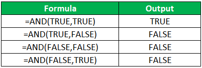
- It returns “true” if all conditions or logical values evaluate to true.
- It returns “false” if any of the conditions or logical values evaluates to false.
- It can have more logical values depending on the situation and the requirement.
- It treats the value zero as “false” and all non-zero values as “true” while evaluating numbers.
- It ignores empty cells provided as an argument.
- It is often used in combination with other Excel functionsExcel functions help the users to save time and maintain extensive worksheets. There are 100+ excel functions categorized as financial, logical, text, date and time, Lookup & Reference, Math, Statistical and Information functions.read more like IF, OR, and so on.
The Output of AND Function
The output in different situations is given as follows:
The output while evaluating numbers is given as follows:
How to Use AND Function in Excel?
It is easy to use the AND function. Let us understand its working with the help of a few examples.
You can download this AND Function Excel Template here – AND Function Excel Template
Example #1–AND Function
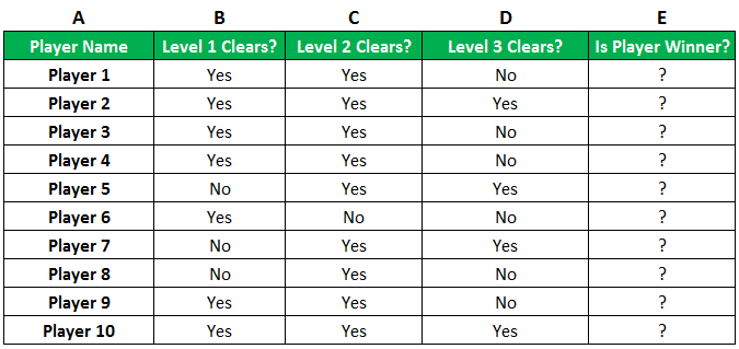
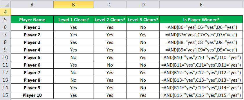
There are three levels and ten players in a game. To be a winner, a player has to clear all three levels. The player loses if he/she fails in any of the three levels.
The performance of the players in different levels is given in the following table. We are required to determine the winner.
We apply AND formula in column E.
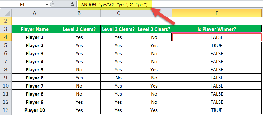
The output of the formula appears in column E.
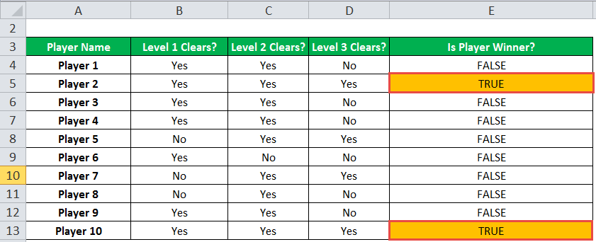
Player 2 and player 10 have cleared all the levels. Since all the logical conditions for these two players are met, the AND function gives the output “true.”
The rest of the players were unable to clear all three levels. If any of the levels is not cleared, the AND function returns “false.”
Example #2–AND Function With Nested IF Function
Let us consider the following example.
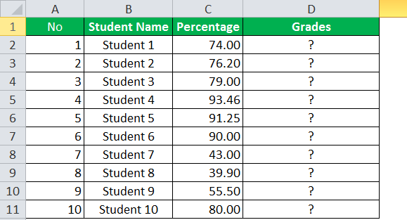
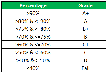
We have the marks (in percentage) of ten students in a school. We have to determine the grade obtained by each student according to the criteria given.
A student obtains “A+” if he/she scores more than 90%. If the percentage is greater than or equal to 80% but less than or equal to 90%, grade “A” is given.
If the percentage is less than 40%, the student fails. Likewise, the grades for the different percentages are given in the following table.
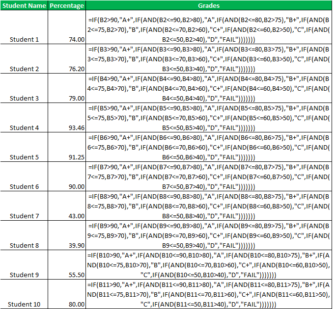
We apply the following formula.
“=IF(B2>90,”A+”,IF(AND(B2<=90,B2>80),”A”,IF(AND(B2<=80,B2>75),”B+”,IF(AND(B2<=75,B2>70),”B”,IF(AND(B2<=70,B2>60),”C+”,IF(AND(B2<=60,B2>50),”C”,IF(AND(B2<=50,B2>40),”D”,”FAIL”)))))))”
We use the nested IF functionIn Excel, nested if function means using another logical or conditional function with the if function to test multiple conditions. For example, if there are two conditions to be tested, we can use the logical functions AND or OR depending on the situation, or we can use the other conditional functions to test even more ifs inside a single if.read more with multiple AND functions to compute the grades. The latter allows testing two conditions together.
The syntax of the IF function is stated as follows:
“=IF(logical_test,[value_if_true],[value_if_false])”
The IF function returns “true” if the condition is met, else returns “false.”
The first logical test is “B2>90.” If this condition is “true,” grade “A+” is assigned. If this condition is “false,” the IF function evaluates the next condition.
The next logical testA logical test in Excel results in an analytical output, either true or false. The equals to operator, “=,” is the most commonly used logical test.read more is “B2<=90, B2>80.” If this condition is “true,” grade “A” is assigned. If this condition is “false,” the next statement is evaluated. Likewise, the IF function tests every condition given in the formula.
The last logical test is “B2<=50, B2>40.” If this condition is “true,” grade “D” is assigned, else the student fails.
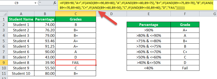
We apply the formula to all categories of students, as shown in the following image.
The output of the formula is shown in the succeeding image.
Example #3–AND Function With Nested IF Function
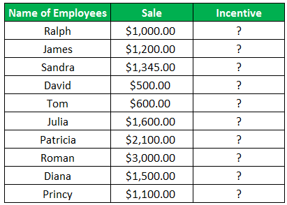
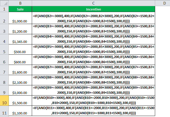
The name of employees and the sales revenueSales revenue refers to the income generated by any business entity by selling its goods or providing its services during the normal course of its operations. It is reported annually, quarterly or monthly as the case may be in the business entity’s income statement/profit & loss account.read more generated by them for an organization are shown in the succeeding image. Every employee is given a monetary incentive depending on the total sales made by him/her.
We have to calculate the incentives of all the employees based on their performance.
The incentive criteria followed by the organization is given in the succeeding table.
We apply the following formula.
“=IF(AND(B2>=3000),400,IF(AND(B2>=2000,B2<3000),200,IF(AND(B2>=1500,B2<2000),150,IF(AND(B2>=1000,B2<1500),100,0))))”
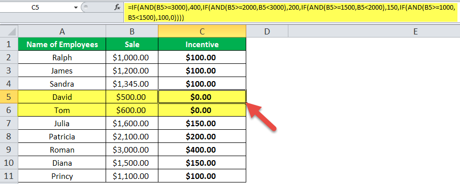
We use multiple IFs In Excel, multiple IF conditions are IF statements that are contained within another IF statement. They are used to test multiple conditions at the same time and return distinct values. Additional IF statements can be included in the ‘value if true’ and ‘value if false’ arguments of a standard IF formula.read moreand multiple AND functions to calculate the incentives received by all the employees, as shown in the following table.
Roman generates sales revenue of $3000. So, he receives an incentive amount of $400.
The revenue generated by David and Tom is $500 and $600, respectively. To be eligible for an incentive, minimum sales of $1000 is required. Hence, they do not get any incentive.
Nesting of AND Function in Excel
A nested function refers to using a function inside another Excel function. In Excel, the nesting of functions up to 64 levels is allowed.
Example #4–Nested AND Function
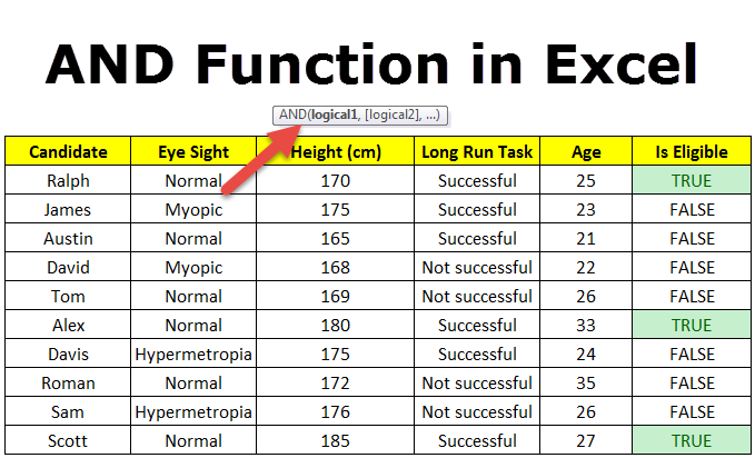
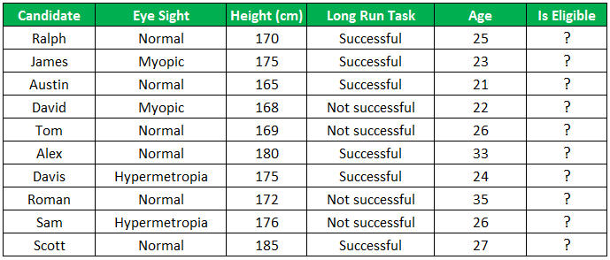
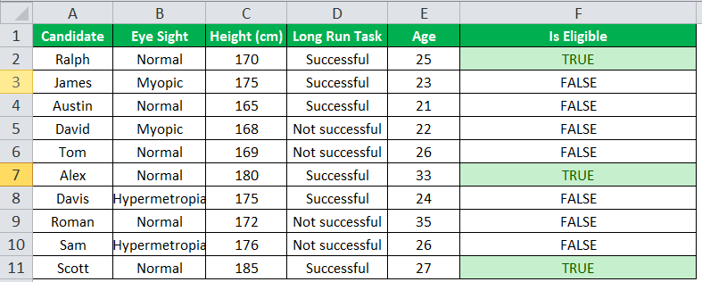
We have a list of candidates who wish to join the Army subject to certain conditions. The eligibility criteria are stated as follows:
- The age should be greater than or equal to 18, but less than 35 years.
- The height should be greater than 167 cm.
- The eyesight should be normal.
- The candidate must have completed the long-run task.
We need to find out the candidates who are eligible for joining the Army.
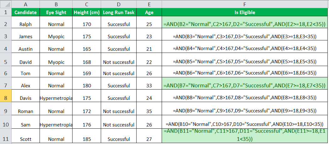
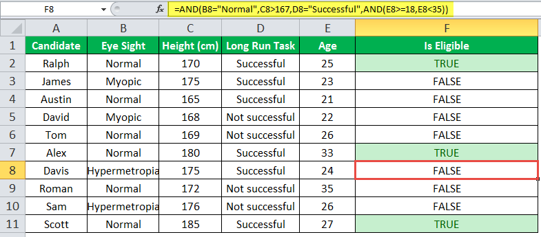
To evaluate the candidates on the given parameters, we use the nested AND function.
We apply the following formula.
“=AND(B2=”Normal”,C2>167,D2=”Successful”,AND(E2>=18,E2<35))”
We evaluate multiple logical conditions simultaneously. We also check whether the age is within the prescribed limit or not. So, we use the AND function inside another AND function.
The output of the formula is shown in the succeeding image.
The candidates Ralph, Alex, and Scott pass the selection criteria. Hence, their eligibility output (in column F) is “true.” The remaining candidates are not eligible for joining the Army.
Limitations of AND Function
The limitations are listed as follows:
- With Excel 2007 onwards, the AND function can test up to 255 arguments given that the length of the formula does not exceed 8,162 characters.
- In Excel 2003 and previous versions, the AND function can test up to 30 arguments given that the length of the formula does not exceed 1,024 characters.
- The AND function returns “#VALUE! error#VALUE! Error in Excel represents that the reference cell the user has either entered an incorrect formula or used a wrong data type (mostly numerical data). Sometimes, it is difficult to identify the kind of mistake behind this error.read more” if logical conditions are passed as text or if none of the arguments evaluates to a logical value.
- The AND function returns “#VALUE! error” if all the arguments provided are empty cells.
The following two images show the output of the AND function when an empty cell and a text string is provided as an argument.
Frequently Asked Questions
#1 – When should the AND function of Excel be used
#2 – How is the AND function used with the OR function in Excel?
The OR function helps compare two values or statements. The AND function is combined with the OR function by the following formulas:
“=AND(OR(Condition1,Condition2),Condition3)”
“=AND(OR(Condition1,Condition2),OR(Condition3,Condition4)”
“=OR(AND(Condition1,Condition2),Condition3)”
“=OR(AND(Condition1,Condition2),AND(Condition3,Condition4))”
#3 – What is the difference between AND, IF, and OR functions in Excel?
The difference between the three functions is stated as follows:
– The AND function helps evaluate multiple conditions at the same time. It returns “true” when all conditions are true; otherwise, it returns “false.”
– The IF function helps compare the value with the result expected by the user. It returns specific values for the “true” and “false” outcomes.
– The OR function helps compare two values or two statements. It returns “true” when at least one of the specified conditions is met. It returns “false” if all the logical values evaluate to false.
- The AND function tests multiple conditions and returns “true” or “false” depending upon whether they are met or not.
- The AND function returns “true” if all conditions evaluate to true and returns “false” if any of the conditions evaluates to false.
- The AND function treats the value zero as “false.”
- The AND function can test up to 255 arguments in the latest versions of Excel.
- The AND function returns “#VALUE! error” if logical conditions are passed as a text.
- The formula of the IF function is “=IF(logical_test,[value_if_true],[value_if_false]).”
Recommended Articles
This has been a guide to AND Function in Excel. Here we discuss how to use AND Formula in Excel along with examples and downloadable excel templates. You may also look at these useful functions in Excel –
- Excel Pivot Table Add ColumnThe pivot table add column helps to add a new column in a pivot table.read more
- Excel Convert FunctionAs the word itself, the Excel CONVERT function defines that it can convert the numbers from one measurement system to another measurement system.read more
- VBA Boolean Data TypeBoolean is an inbuilt data type in VBA used for logical references or logical variables. The value this data type holds is either TRUE or FALSE and is used for logical comparison. The declaration of this data type is similar to all the other data types.read more
- IF AND Formula in ExcelThe IF AND excel formula is the combination of two different logical functions often nested together that enables the user to evaluate multiple conditions using AND functions. Based on the output of the AND function, the IF function returns either the “true” or “false” value, respectively.
read more
This post will guide you how to use IF function combining with AND logical function in Excel.
If you want to check if a value in cell match two or more conditions at the same time, if the test is TRUE, then you can take certain action. You can use the IF function combining with AND function to construct a condition statement. If the test is FALSE, then take another action.
Table of Contents
- Excel formula using IF & AND function
- Related Formulas
- Related Functions
The syntax of AND function in excel is as follow:
=AND(condition1,[condition2],...)
The Excel AND function returns TRUE if all of arguments are TRUE, and it returns FALSE if any of arguments are FALSE.
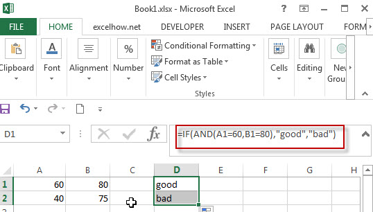
Now we want to check the results of two exam scores where the first score in cell A1 is greater than or equal to 60 AND the second score in cell B1 is greater than or equal to 80. If both conditions are TRUE, then returns the text of “good”, and if FALSE returns “bad”. Based on the above logic, we can write down the below IF formula:
=IF(AND(A1=60,B1=80),"good","bad")
We can enter the above formula into cell D1, and then drag the Fill Handle to the range D1:D3.it will apply for the other cells for this formula.
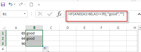
The logic test will check the two different cells in the above IF formula, if we can run two or more tests on the same cell. Of course yes, for example, if you want to check cell A1 if the value in cell A1 is greater than 60 but less than or equal to 70. If the test is TRUE, then take one action.
The logical test we can use for above logic as below:
=AND(A1>60, A1<=70)
IF formula:
=IF(AND(A1>60,A1<=70),”good”,””)
In this formula, if the test is FALSE, we just add an empty string (“”), IF the test is TRUE, the test string of “good” will appear.
Note: The AND function will check all test conditions in excel, even if one of the already tested conditions has a value of FALSE. This behavior is different with other programming languages. If any previous test conditions return FALSE, the subsequent conditions will not be tested.
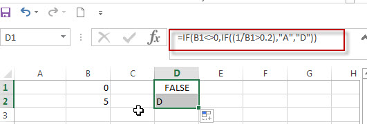
For example: If the value of Cell B1 is 0, then the below IF&AND formula will return error message as “Divide by Zero Error”.
=IF(AND(B1<>0,(1/B1)>0.2),”A”,”D”))
As mentioned above, the AND function will check all conditions. To avoid this issue, we can use a nested IF function and check if the value of Cell B1 is not equal to 0 in the first IF statement.
The nested if formula is as below:
=IF(B1<>0,IF((1/B1>0.2),”A”,”D”))
- Excel IF formula with equal to logical operator
The “Equal to” logical operator can be used to compare the below data types, such as: text string, numbers, dates, Booleans. This section will guide you how to use “equal to” logical operator in excel IF formula with text string value and dates value… - Excel IF formula with OR logical function
If you want to check if one of several conditions is met in your excel workbook, if the test is TRUE, then you can take certain action. You can use the IF function combining with OR function to construct a condition statement… - Excel IF formula with AND & OR logical functions
If you want to test the result of cells based on several sets of multiple test conditions, you can use the IF function with the AND and OR functions at a time…
- Excel AND function
The Excel AND function returns TRUE if all of arguments are TRUE, and it returns FALSE if any of arguments are FALSE.The syntax of the AND function is as below:= AND (condition1,[condition2],…) … - Excel IF function
The Excel IF function perform a logical test to return one value if the condition is TRUE and return another value if the condition is FALSE…. - Excel nested if function
The nested IF function is formed by multiple if statements within one Excel if function. This excel nested if statement makes it possible for a single formula to take multiple actions…
Brief syntax lesson
Cells(Row, Column) identifies a cell. Row must be an integer between 1 and the maximum for version of Excel you are using. Column must be a identifier (for example: «A», «IV», «XFD») or a number (for example: 1, 256, 16384)
.Cells(Row, Column) identifies a cell within a sheet identified in a earlier With statement:
With ActiveSheet
  :
  .Cells(Row,Column)
  :
End With
If you omit the dot, Cells(Row,Column) is within the active worksheet. So wsh = ActiveWorkbook wsh.Range is not strictly necessary. However, I always use a With statement so I do not wonder which sheet I meant when I return to my code in six months time. So, I would write:
With ActiveSheet
  :
  .Range.
  :
End With
Actually, I would not write the above unless I really did want the code to work on the active sheet. What if the user has the wrong sheet active when they started the macro. I would write:
With Sheets("xxxx")
  :
  .Range.
  :
End With
because my code only works on sheet xxxx.
Cells(Row,Column) identifies a cell. Cells(Row,Column).xxxx identifies a property of the cell. Value is a property. Value is the default property so you can usually omit it and the compiler will know what you mean. But in certain situations the compiler can be confused so the advice to include the .Value is good.
Cells(Row,Column) like "*Miami*" will give True if the cell is «Miami», «South Miami», «Miami, North» or anything similar.
Cells(Row,Column).Value = "Miami" will give True if the cell is exactly equal to «Miami». «MIAMI» for example will give False. If you want to accept MIAMI, use the lower case function:
Lcase(Cells(Row,Column).Value) = "miami"
My suggestions
Your sample code keeps changing as you try different suggestions which I find confusing. You were using Cells(Row,Column) <> "Miami" when I started typing this.
Use
If Cells(i, "A").Value like "*Miami*" And Cells(i, "D").Value like "*Florida*" Then
  Cells(i, "C").Value = "BA"
if you want to accept, for example, «South Miami» and «Miami, North».
Use
If Cells(i, "A").Value = "Miami" And Cells(i, "D").Value like "Florida" Then
  Cells(i, "C").Value = "BA"
if you want to accept, exactly, «Miami» and «Florida».
Use
If Lcase(Cells(i, "A").Value) = "miami" And _
   Lcase(Cells(i, "D").Value) = "florida" Then
  Cells(i, "C").Value = "BA"
if you don’t care about case.
To write an IF, AND, OR array formula in Excel 365, we must use the arithmetic operators * (multiplication) and + (addition). Why it’s so?
If we take the logical AND, OR with the IF in Excel 365 to spill the result, we won’t get our expected result.
I mean, such a formula won’t support a range/array in evaluation. Even if it supports, it won’t return an array result.
So we will replace the AND logical operator with the * (multiplication) and OR with the + (addition) arithmetic operators.
Coding the formula with the said two operators is very simple and easily readable.
I think I can convince you the same with the examples below.
Example to IF, AND, OR in Excel 365 (Non-Array Formula)
Imagine a user played a game three times, and we have recorded his scores out of 100 in cells A2, B2, and C2.
We want to perform the following three logical tests on the scores individually.
- If all scores are >=80, return OK.
- If any of the two scores are >=80, return OK.
- Finally, if any of the scores is >=80, return OK.
Logical Tests Using IF, AND, OR Functions
In Excel, we can perform the above three logical tests as follows.
1. E2 (If all scores are >=80, return OK)
=IF(AND(A2>=80,B2>=80,C2>=80),"OK","NOT OK")I have used the AND function with IF in the above Excel formula to test if all the three logical tests return TRUE.
2. F2 (If any of the two scores are >=80, return OK)
We must use the following logic (two parts) to test if any two logical tests return TRUE.
AND Part:-
a) Value 1>=80 and value 2>=80.
b) Value 1>=80 and value 3>=80.
c) Value 2>=80 and value 3>=80.
OR Part:-
a) The OR evaluates to TRUE if any two of the above three AND tests return TRUE.
So the formula will be as follows.
=IF(OR(AND(A2>=80,B2>=80),AND(A2>=80,C2>=80),AND(B2>=80,C2>=80)),"OK","NOT OK")It is an example of the IF, AND, OR logical test in Excel.
3. G2 (if any of the scores is >=80, return OK)
=IF(OR(A2>=80,B2>=80,C2>=80),"OK","NOT OK")Here I have used the OR function with IF to test if any of the three logical tests return TRUE.
As I have already mentioned, we can’t write an IF, AND, OR array formula as above in Excel 365.
Logical Tests Using IF, *, + Formula
Let’s substitute the above three formulas by replacing AND, OR with multiplication and addition.
But that’s not enough. Then?
The below formulas are self-explanatory.
1. E2 Formula
=IF((A2:A8>=80)*(B2:B8>=80)*(C2:C8>=80),"OK","NOT OK")How the multiplication replaces the logical function OR above?
Each test in the formula returns either TRUE or FALSE. If all the criteria are met, it will be =IF((TRUE*TRUE*TRUE),"OK","NOT OK").
We can even replace the multiplication operator here with addition.
=IF((A2:A8>=80)+(B2:B8>=80)+(C2:C8>=80)>2,"OK","NOT OK")Please remember that the value of TRUE is 1, and FALSE is 0.
2. F2 Formula
=IF((A2:A8>=80)+(B2:B8>=80)+(C2:C8>=80)>1,"OK","NOT OK")3. G2 Formula
=IF((A2:A8>=80)+(B2:B8>=80)+(C2:C8>=80)>0,"OK","NOT OK")Above I have tried to simplify the use of the logical operators within the IF function.
Now let’s open an Excel Spreadsheet and enter the scores of multiple players in the range A2:C8 as below.
So the values to evaluate are in cell range A2:C8.
I have inserted the following three IF, AND, OR array formulas in cells E2, F2, and G2, respectively.
1. E2 Array Formula
=IF((A2:A8>=80)*(B2:B8>=80)*(C2:C8>=80),"OK","NOT OK")2. F2 Array Formula
=IF((A2:A8>=80)+(B2:B8>=80)+(C2:C8>=80)>1,"OK","NOT OK")3. G2 Array Formula
=IF((A2:A8>=80)+(B2:B8>=80)+(C2:C8>=80)>0,"OK","NOT OK")If any of the above formulas return #SPILL!, please empty the cells down in that column.
Nested IF, AND, OR Combination in Excel 365
I want to assign grades based on the scores above.
In that case, we may require to write a nested IF, AND, OR combination array formula in Excel 365.
Here is how.
In the above example, we have used three formulas for the below three logical tests.
- If all scores are >=80, return OK.
- If any of the two scores are >=80, return OK.
- Finally, if any of the scores is >=80, return OK.
There each test returns OK or NOT OK.
Instead of that, here, I want the tests to return GR-1, GR-2, and GR-3.
- If all scores are >=80, return GR-1.
- If any of the two scores are >=80, return GR-2.
- Finally, if any of the scores is >=80, return GR-3.
For that, we should combine the above three IF, AND, OR Array Formulas.
How?
In the E2 formula, replace “OK” with “GR-1” and “NOT OK” with the F2 formula.
In that combined (E2 and F2) formula, replace “OK” with “GR-2” and “NOT OK” with the G2 formula.
Then, in the combined E2, F2, and G2 formula, replace “OK” with “GR-3” and replace “NOT OK” with “F.”
Here it is.
=IF(
     (A2:A8>=80)*(B2:B8>=80)*(C2:C8>=80),"GR-1",
     IF(
        (A2:A8>=80)+(B2:B8>=80)+(C2:C8>=80)>1,"GR-2",
        IF(
           (A2:A8>=80)+(B2:B8>=80)+(C2:C8>=80)>0,"GR-3","F"
        )
     )
)
We can call it a nested IF, AND, OR combination array formula.
Related:- How to Use the IFS Function in Excel 365.
Home / Excel Formulas / How to Combine IF and AND Functions in Excel
As I told you, by combining IF with other functions you can increase its powers. AND function is one of the most useful functions to combine with the IF function.
Like you combine IF and OR functions to test multiple conditions. In the same way, you can combine IF and AND functions.
There is a slight difference in using OR, and AND functions with IF. In this post, you will learn to combine IF & AND functions and you will also learn why we need to combine both of these.
Quick Intro
Both of these functions are useful but by using them jointly, you can solve some real-life problems. Here is a quick intro for both.
- IF Function – To test a condition and return a specific value if that condition is true or another specific value if that condition is false.
- AND Function – To test multiple conditions. If all the conditions are true then it will return true and if any of the conditions are false then it will return false.
Why is this Important?
- You can test more than one condition with the IF function.
- It will return a specific value if all the conditions are true.
- Or, it will return another specific value if any of the conditions are false.
How do IF and AND Functions Work?
To combine IF and AND functions you have to just replace the logical_test argument in the IF function with AND function. By using AND function you can specify more than one condition.

Now AND function will test your all conditions here. If all the conditions are true then AND function will return true and the IF function will return the value which you have specified for true.
And, if any of the conditions is false then AND function will return false, and the IF function will return the value which you have specified for false. Let me show you a real-life example.
Examples
Here I have a marks sheet of students. And, I want to add some remarks to the sheet.

If a student is passed both of the subjects with 40 marks or above, the status should be “Pass”. And, if a student has less than 40 marks in both of the subjects or even in one subject, the status should be “Fail”. The formula will be.
=IF(AND(B2>=40,C2>=40),"Pass","Fail")
In the above formula, if there is a value 40 or greater than in any of the cells (B2 & C2) AND function will return true, and IF will return the value “Pass”. That means if a student passed both of the subjects then he/she will pass.
But, if both cells have a value lower than 40 then AND will return false, and IF will return the value “Fail”. If a student is failed in any of the subjects he/she will fail.
Download Sample File
- Ready
And, if you want to Get Smarter than Your Colleagues check out these FREE COURSES to Learn Excel, Excel Skills, and Excel Tips and Tricks.
Excel IF AND OR functions on their own aren’t very exciting, but mix them up with the IF Statement and you’ve got yourself a formula that’s much more powerful.
In this tutorial we’re going to take a look at the basics of the AND and OR functions and then put them to work with an IF Statement. If you aren’t familiar with IF Statements, click here to read that tutorial first.
IF Formula Builder
Our IF Formula Builder does the hard work of creating IF formulas.
You just need to enter a few pieces of information, and the workbook creates the formula for you.
AND Function
The AND function belongs to the logic family of formulas, along with IF, OR and a few others. It’s useful when you have multiple conditions that must be met.
In Excel language on its own the AND formula reads like this:
=AND(logical1,[logical2]....)
Now to translate into English:
=AND(is condition 1 true, AND condition 2 true (add more conditions if you want)
OR Function
The OR function is useful when you are happy if one, OR another condition is met.
In Excel language on its own the OR formula reads like this:
=OR(logical1,[logical2]....)
Now to translate into English:
=OR(is condition 1 true, OR condition 2 true (add more conditions if you want)
See, I did say they weren’t very exciting, but let’s mix them up with IF and put AND and OR to work.
IF AND Formula
First let’s set the scene of our challenge for the IF, AND formula:
In our spreadsheet below we want to calculate a bonus to pay the children’s TV personalities listed. The rules, as devised by my 4 year old son, are:
1) If the TV personality is Popular AND
2) If they earn less than $100k per year they get a 10% bonus (my 4 year old will write them an IOU, he’s good for it though).

In cell D2 we will enter our IF AND formula as follows:
In English first
=IF(Spider Man is Popular, AND he earns <$100k), calculate his salary x 10%, if not put "Nil" in the cell)
Now in Excel’s language:
=IF(AND(B2="Yes",C2<100),C2x$H$1,"Nil")
You’ll notice that the two conditions are typed in first, and then the outcomes are entered. You can have more than two conditions; in fact you can have up to 30 by simply separating each condition with a comma (see warning below about going overboard with this though).
IF OR Formula
Again let’s set the scene of our challenge for the IF, OR formula:
The revised rules, as devised by my 4 year old son, are:
1) If the TV personality is Popular OR
2) If they earn less than $100k per year they get a 10% bonus.

In cell D2 we will enter our IF OR formula as follows:
In English first
=IF(Spider Man is Popular, OR he earns <$100k), calculate his salary x 10%, if not put “Nil” in the cell)
Now in Excel’s language:
=IF(OR(B2="Yes",C2<100),C2x$H$1,"Nil")
Notice how a subtle change from the AND function to the OR function has a significant impact on the bonus figure.
Just like the AND function, you can have up to 30 OR conditions nested in the one formula, again just separate each condition with a comma.
Try other operators
You can set your conditions to test for specific text, as I have done in this example with B2=»Yes», just put the text you want to check between inverted comas “ ”.
Alternatively you can test for a number and because the AND and OR functions belong to the logic family, you can employ different tests other than the less than (<) operator used in the examples above.
Other operators you could use are:
- = Equal to
- > Greater Than
- <= Less than or equal to
- >= Greater than or equal to
- <> Less than or greater than
Warning: Don’t go overboard with nesting IF, AND, and OR’s, as it will be painful to decipher if you or someone else ever needs to update the formula in months or years to come.
Note: These formulas work in all versions of Excel, however versions pre Excel 2007 are limited to 7 nested IF’s.
Download the Workbook
Enter your email address below to download the sample workbook.
By submitting your email address you agree that we can email you our Excel newsletter.
Excel IF AND OR Practice Questions
IF AND Formula Practice
In the embedded Excel workbook below insert a formula (in the grey cells in column E), that returns the text ‘Yes’, when a product SKU should be reordered, based on the following criteria:
- If Stock on hand is less than 20,000 AND
- Demand level is ‘High’
If the above conditions are met, return ‘Yes’, otherwise, return ‘No’.
Tips for working with the embedded workbook:
- Use arrow keys to move around the worksheet when you can’t click on the cells with your mouse
- Use shortcut keys CTRL+C to copy and CTRL+V to paste
- Don’t forget to absolute cell references where applicable
- Do not enter anything in column F
- Double click to edit a cell
- Refresh the page to reset the embedded workbook
IF OR Formula Practice
In the embedded Excel workbook below insert a formula (in the grey cells in column E) that calculates the bonus due for each salesperson. A $500 bonus is paid if a salesperson meets either target in cells C24 and C25, otherwise they earn $0 bonus.
Want More Excel Formulas
Why not visit our list of Excel formulas. You’ll find a huge range all explained in plain English, plus PivotTables and other Excel tools and tricks. Enjoy 🙂


