And if functions in excel examples - Word и Excel - помощь в работе с программами

The IF function allows you to make a logical comparison between a value and what you expect by testing for a condition and returning a result if that condition is True or False.

=IF(Something is True, then do something, otherwise do something else)

But what if you need to test multiple conditions, where let’s say all conditions need to be True or False (AND), or only one condition needs to be True or False (OR), or if you want to check if a condition does NOT meet your criteria? All 3 functions can be used on their own, but it’s much more common to see them paired with IF functions.

Use the IF function along with AND, OR and NOT to perform multiple evaluations if conditions are True or False.

Syntax

IF(AND()) — IF(AND(logical1, [logical2], …), value_if_true, [value_if_false]))
IF(OR()) — IF(OR(logical1, [logical2], …), value_if_true, [value_if_false]))
IF(NOT()) — IF(NOT(logical1), value_if_true, [value_if_false]))


Argument name	Description
logical_test (required)	The condition you want to test.
value_if_true (required)	The value that you want returned if the result of logical_test is TRUE.

value_if_false (optional)	The value that you want returned if the result of logical_test is FALSE.

Here are overviews of how to structure AND, OR and NOT functions individually. When you combine each one of them with an IF statement, they read like this:

AND – =IF(AND(Something is True, Something else is True), Value if True, Value if False)
OR – =IF(OR(Something is True, Something else is True), Value if True, Value if False)
NOT – =IF(NOT(Something is True), Value if True, Value if False)

Examples

Following are examples of some common nested IF(AND()), IF(OR()) and IF(NOT()) statements. The AND and OR functions can support up to 255 individual conditions, but it’s not good practice to use more than a few because complex, nested formulas can get very difficult to build, test and maintain. The NOT function only takes one condition.

Here are the formulas spelled out according to their logic:

Formula	Description
=IF(AND(A2>0,B2<100),TRUE, FALSE)	IF A2 (25) is greater than 0, AND B2 (75) is less than 100, then return TRUE, otherwise return FALSE. In this case both conditions are true, so TRUE is returned.
=IF(AND(A3=»Red»,B3=»Green»),TRUE,FALSE)	If A3 (“Blue”) = “Red”, AND B3 (“Green”) equals “Green” then return TRUE, otherwise return FALSE. In this case only the first condition is true, so FALSE is returned.
=IF(OR(A4>0,B4<50),TRUE, FALSE)	IF A4 (25) is greater than 0, OR B4 (75) is less than 50, then return TRUE, otherwise return FALSE. In this case, only the first condition is TRUE, but since OR only requires one argument to be true the formula returns TRUE.
=IF(OR(A5=»Red»,B5=»Green»),TRUE,FALSE)	IF A5 (“Blue”) equals “Red”, OR B5 (“Green”) equals “Green” then return TRUE, otherwise return FALSE. In this case, the second argument is True, so the formula returns TRUE.
=IF(NOT(A6>50),TRUE,FALSE)	IF A6 (25) is NOT greater than 50, then return TRUE, otherwise return FALSE. In this case 25 is not greater than 50, so the formula returns TRUE.
=IF(NOT(A7=»Red»),TRUE,FALSE)	IF A7 (“Blue”) is NOT equal to “Red”, then return TRUE, otherwise return FALSE.

Note that all of the examples have a closing parenthesis after their respective conditions are entered. The remaining True/False arguments are then left as part of the outer IF statement. You can also substitute Text or Numeric values for the TRUE/FALSE values to be returned in the examples.

Here are some examples of using AND, OR and NOT to evaluate dates.

Here are the formulas spelled out according to their logic:

Formula	Description
=IF(A2>B2,TRUE,FALSE)	IF A2 is greater than B2, return TRUE, otherwise return FALSE. 03/12/14 is greater than 01/01/14, so the formula returns TRUE.
=IF(AND(A3>B2,A3<C2),TRUE,FALSE)	IF A3 is greater than B2 AND A3 is less than C2, return TRUE, otherwise return FALSE. In this case both arguments are true, so the formula returns TRUE.
=IF(OR(A4>B2,A4<B2+60),TRUE,FALSE)	IF A4 is greater than B2 OR A4 is less than B2 + 60, return TRUE, otherwise return FALSE. In this case the first argument is true, but the second is false. Since OR only needs one of the arguments to be true, the formula returns TRUE. If you use the Evaluate Formula Wizard from the Formula tab you’ll see how Excel evaluates the formula.
=IF(NOT(A5>B2),TRUE,FALSE)	IF A5 is not greater than B2, then return TRUE, otherwise return FALSE. In this case, A5 is greater than B2, so the formula returns FALSE.

Using AND, OR and NOT with Conditional Formatting

You can also use AND, OR and NOT to set Conditional Formatting criteria with the formula option. When you do this you can omit the IF function and use AND, OR and NOT on their own.

From the Home tab, click Conditional Formatting > New Rule. Next, select the “Use a formula to determine which cells to format” option, enter your formula and apply the format of your choice.

Using the earlier Dates example, here is what the formulas would be.

Formula	Description
=A2>B2	If A2 is greater than B2, format the cell, otherwise do nothing.
=AND(A3>B2,A3<C2)	If A3 is greater than B2 AND A3 is less than C2, format the cell, otherwise do nothing.
=OR(A4>B2,A4<B2+60)	If A4 is greater than B2 OR A4 is less than B2 plus 60 (days), then format the cell, otherwise do nothing.
=NOT(A5>B2)	If A5 is NOT greater than B2, format the cell, otherwise do nothing. In this case A5 is greater than B2, so the result will return FALSE. If you were to change the formula to =NOT(B2>A5) it would return TRUE and the cell would be formatted.

Note: A common error is to enter your formula into Conditional Formatting without the equals sign (=). If you do this you’ll see that the Conditional Formatting dialog will add the equals sign and quotes to the formula — =»OR(A4>B2,A4<B2+60)», so you’ll need to remove the quotes before the formula will respond properly.

Need more help?

Examples of using formulas with IF, AND, OR functions in Excel

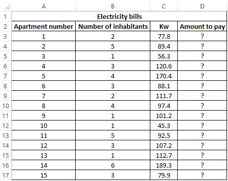
Example 1. When calculating the cost of the amount of consumed kW of electricity for subscribers, the following conditions are taken into account:

If less than 3 people live in the apartment or less than 100 kW of electricity was consumed per month, the rate per 1 kW is 4.35$.
In other cases, the rate for 1 kW is 5.25$.

Calculate the amount payable per month for several subscribers.

View source data table:

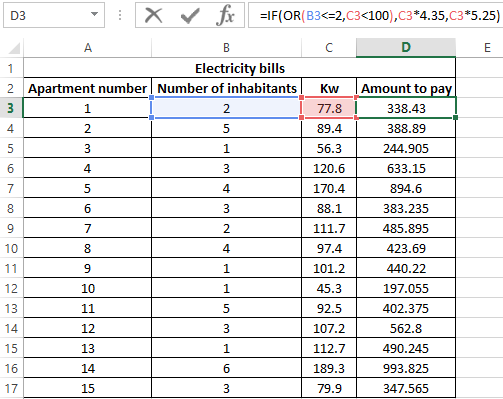
Perform the calculation according to the formula:

Argument Description:

OR (B3<=2,C3<100) is a logical expression that verifies two conditions: do less than 3 people live in the apartment or does the total amount of energy consumed less than 100 kW? The result of the test will be TRUE if either of these two conditions is true;
C3 * 4.35 — the amount to be paid, if the OR function returns TRUE;
C3 * 5.25 is the amount to be paid if OR returns FALSE.

We stretch the formula for the remaining cells using the autocomplete function. The result of the calculation for each subscriber:

Using the AND function in the formula in the first argument in the IF function, we check the conformity of the values by two conditions at once.

Formula with IF and AVERAGE functions for selecting of values by conditions

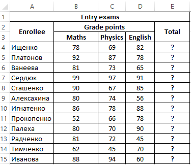
Example 2. Applicants entering the university for the specialty «mechanical engineer» are required to pass 3 exams in mathematics, physics and English. The maximum score for each exam is 100. The average passing score for 3 exams is 75, while the minimum score in physics must be at least 70 points, and in mathematics it is 80. Determine applicants who have successfully passed the exams.

View source table:

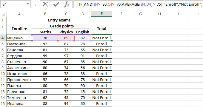
To determine the enrolled students use the formula:

Argument Description:

AND(B4>=80,C4>=70,AVERAGE(B4:D4)>=75) — checked logical expressions according to the condition of the problem;
«Enroll» — the result, if the function AND returned the value TRUE (all expressions represented as its arguments, as a result of the calculations returned the value TRUE);
«Not Enroll» — the result if AND returned FALSE.

Using the autocomplete function (double-click on the cursor marker in the lower right corner), we get the rest of the results:

Formula with logical functions AND IF OR in excel

Example 3. Subsidies in the amount of 30% are charged to families with an average income below 8,000$, which are large or there is no main breadwinner. If the number of children is over 5, the amount of the subsidy is 50%. Determine who should receive subsidies and who should not.

View source table:

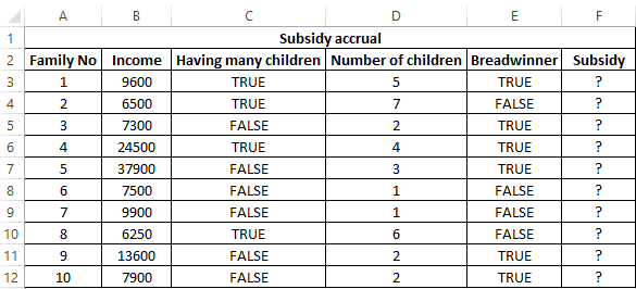
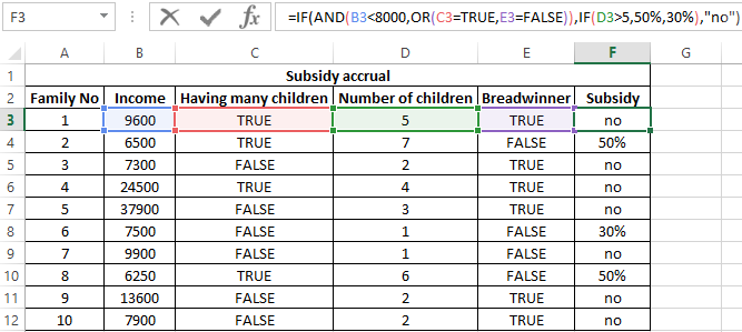
To check the criteria according to the condition of the problem, we write the formula:

Argument Description:

AND(B3<8000,OR(C3=TRUE,E3=FALSE)) is the checked expression according to the condition of the problem. In this case, the AND function returns the TRUE value, if B3 <8000 is true and at least one of the expressions passed as arguments to the OR function also returns the TRUE value.
The nested IF function performs a check on the number of children in the family, which rely on subsidies.
If the main condition returned the result is FALSE, the main function IF returns the text string “no”.

Perform the calculation for the first family and stretch the formula to the remaining cells using the autocomplete function. Results:

Features of using logical functions IF, AND, OR in Excel

The IF function has the following syntax notation:

=IF(Logical_test,[ Value_if_True ],[ Value_if_False])

As you can see, by default, you can check only one condition, for example, is e3 more than 20? Using the IF function, this check can be done as follows:

=IF(EXP(3)>20,»more»,»less»)

As a result, the text string “more” will be returned. If we need to find out if any value belongs to the specified interval, we will need to compare this value with the upper and lower limits of the intervals, respectively. For example, is the result of calculating e3 in the range from 20 to 25? When using the IF function alone, you must enter the following entry:

=IF(EXP(3)>20,IF(EXP(3)<25,»belongs»,»does not belong»),»does not belong»)

We have a nested function IF as one of the possible results of the implementation of the main function IF, and therefore the syntax looks somewhat cumbersome. If you also need to know, for example, whether the square root e3 is equal to a numeric value from a fractional number range from 4 to 5, the final formula will look cumbersome and unreadable.

It is much easier to use as a condition a complex expression that can be written using AND and OR functions. For example, the above function can be rewritten as follows:

=IF(AND(EXP(3)>20,EXP(3)<25),»belongs»,»does not belong»)

The result of the execution of the AND expression (EXP(3)>20,EXP(3)<25) can be a logical value TRUE only if the result of checking each of the specified conditions is a logical value TRUE. In other words, the function AND allows you to test one, two or more hypotheses on their truth, and returns the result FALSE if at least one of them is incorrect.

Sometimes you want to know if at least one assumption is true. In this case, it is convenient to use the OR function, which performs the check of one or several logical expressions and returns a logical TRUE, if the result of the calculations of at least one of them is a logical TRUE. For example, you want to know if e3 is an integer or a number that is less than 100? To test this condition, you can use the following formula:

=IF(OR(MOD(EXP(3),1)<>0,EXP(3)<100),»true»,»false»)

The “<>” means inequality, that is, more or less than some value. In this case, both expressions return the value TRUE, and the result of the execution of the IF function is the text string «true.» However, if an OR test was performed (MOD(EXP (3),1)<>0,EXP(3)<20, while EXP(3) <20 will return FALSE, the result of the calculation of the IF function will not change, since MOD(EXP(3),1) <> 0 returns TRUE.

Download examples using the functions OR AND IF in Excel

In practice, often used bundles IF + AND, IF + OR, or all three functions at once. Consider examples of similar use of these functions.

Источник

Функция ЕСЛИ в Excel — это отличный инструмент для проверки условий на ИСТИНУ или ЛОЖЬ. Если значения ваших расчетов равны заданным параметрам функции как ИСТИНА, то она возвращает одно значение, если ЛОЖЬ, то другое.

Содержание

Что возвращает функция
Синтаксис
Аргументы функции
Дополнительная информация
Функция Если в Excel примеры с несколькими условиями
Пример 1. Проверяем простое числовое условие с помощью функции IF (ЕСЛИ)
Пример 2. Использование вложенной функции IF (ЕСЛИ) для проверки условия выражения
Пример 3. Вычисляем сумму комиссии с продаж с помощью функции IF (ЕСЛИ) в Excel
Пример 4. Используем логические операторы (AND/OR) (И/ИЛИ) в функции IF (ЕСЛИ) в Excel
Пример 5. Преобразуем ошибки в значения “0” с помощью функции IF (ЕСЛИ)

Что возвращает функция

Заданное вами значение при выполнении двух условий ИСТИНА или ЛОЖЬ.

Синтаксис

=IF(logical_test, [value_if_true], [value_if_false]) — английская версия

=ЕСЛИ(лог_выражение; [значение_если_истина]; [значение_если_ложь]) — русская версия

Аргументы функции

logical_test (лог_выражение) — это условие, которое вы хотите протестировать. Этот аргумент функции должен быть логичным и определяемым как ЛОЖЬ или ИСТИНА. Аргументом может быть как статичное значение, так и результат функции, вычисления;
[value_if_true] ([значение_если_истина]) — (не обязательно) — это то значение, которое возвращает функция. Оно будет отображено в случае, если значение которое вы тестируете соответствует условию ИСТИНА;
[value_if_false] ([значение_если_ложь]) — (не обязательно) — это то значение, которое возвращает функция. Оно будет отображено в случае, если условие, которое вы тестируете соответствует условию ЛОЖЬ.

Дополнительная информация

В функции ЕСЛИ может быть протестировано 64 условий за один раз;
Если какой-либо из аргументов функции является массивом — оценивается каждый элемент массива;
Если вы не укажете условие аргумента FALSE (ЛОЖЬ) value_if_false (значение_если_ложь) в функции, т.е. после аргумента value_if_true (значение_если_истина) есть только запятая (точка с запятой), функция вернет значение “0”, если результат вычисления функции будет равен FALSE (ЛОЖЬ).
На примере ниже, формула =IF(A1> 20,”Разрешить”) или =ЕСЛИ(A1>20;»Разрешить») , где value_if_false (значение_если_ложь) не указано, однако аргумент value_if_true (значение_если_истина) по-прежнему следует через запятую. Функция вернет “0” всякий раз, когда проверяемое условие не будет соответствовать условиям TRUE (ИСТИНА).

|
Если вы не укажете условие аргумента TRUE(ИСТИНА) (value_if_true (значение_если_истина)) в функции, т.е. условие указано только для аргумента value_if_false (значение_если_ложь), то формула вернет значение “0”, если результат вычисления функции будет равен TRUE (ИСТИНА);
На примере ниже формула равна =IF (A1>20;«Отказать») или =ЕСЛИ(A1>20;»Отказать»), где аргумент value_if_true (значение_если_истина) не указан, формула будет возвращать “0” всякий раз, когда условие соответствует TRUE (ИСТИНА).

Функция Если в Excel примеры с несколькими условиями

Пример 1. Проверяем простое числовое условие с помощью функции IF (ЕСЛИ)

При использовании функции ЕСЛИ в Excel, вы можете использовать различные операторы для проверки состояния. Вот список операторов, которые вы можете использовать:

Ниже приведен простой пример использования функции при расчете оценок студентов. Если сумма баллов больше или равна «35», то формула возвращает “Сдал”, иначе возвращается “Не сдал”.

Пример 2. Использование вложенной функции IF (ЕСЛИ) для проверки условия выражения

Функция может принимать до 64 условий одновременно. Несмотря на то, что создавать длинные вложенные функции нецелесообразно, то в редких случаях вы можете создать формулу, которая множество условий последовательно.

В приведенном ниже примере мы проверяем два условия.

Первое условие проверяет, сумму баллов не меньше ли она чем 35 баллов. Если это ИСТИНА, то функция вернет “Не сдал”;
В случае, если первое условие — ЛОЖЬ, и сумма баллов больше 35, то функция проверяет второе условие. В случае если сумма баллов больше или равна 75. Если это правда, то функция возвращает значение “Отлично”, в других случаях функция возвращает “Сдал”.

Пример 3. Вычисляем сумму комиссии с продаж с помощью функции IF (ЕСЛИ) в Excel

Функция позволяет выполнять вычисления с числами. Хороший пример использования — расчет комиссии продаж для торгового представителя.

В приведенном ниже примере, торговый представитель по продажам:

не получает комиссионных, если объем продаж меньше 50 тыс;
получает комиссию в размере 2%, если продажи между 50-100 тыс
получает 4% комиссионных, если объем продаж превышает 100 тыс.

Рассчитать размер комиссионных для торгового агента можно по следующей формуле:

=IF(B2<50,0,IF(B2<100,B2*2%,B2*4%)) — английская версия

=ЕСЛИ(B2<50;0;ЕСЛИ(B2<100;B2*2%;B2*4%)) — русская версия

В формуле, использованной в примере выше, вычисление суммы комиссионных выполняется в самой функции ЕСЛИ. Если объем продаж находится между 50-100K, то формула возвращает B2 * 2%, что составляет 2% комиссии в зависимости от объема продажи.

Больше лайфхаков в нашем Telegram Подписаться

Пример 4. Используем логические операторы (AND/OR) (И/ИЛИ) в функции IF (ЕСЛИ) в Excel

Вы можете использовать логические операторы (AND/OR) (И/ИЛИ) внутри функции для одновременного тестирования нескольких условий.

Например, предположим, что вы должны выбрать студентов для стипендий, основываясь на оценках и посещаемости. В приведенном ниже примере учащийся имеет право на участие только в том случае, если он набрал более 80 баллов и имеет посещаемость более 80%.

Вы можете использовать функцию AND (И) вместе с функцией IF (ЕСЛИ), чтобы сначала проверить, выполняются ли оба эти условия или нет. Если условия соблюдены, функция возвращает “Имеет право”, в противном случае она возвращает “Не имеет право”.

Формула для этого расчета:

=IF(AND(B2>80,C2>80%),”Да”,”Нет”) — английская версия

=ЕСЛИ(И(B2>80;C2>80%);»Да»;»Нет») — русская версия

Пример 5. Преобразуем ошибки в значения “0” с помощью функции IF (ЕСЛИ)

С помощью этой функции вы также можете убирать ячейки содержащие ошибки. Вы можете преобразовать значения ошибок в пробелы или нули или любое другое значение.

Формула для преобразования ошибок в ячейках следующая:

=IF(ISERROR(A1),0,A1) — английская версия

=ЕСЛИ(ЕОШИБКА(A1);0;A1) — русская версия

Формула возвращает “0”, в случае если в ячейке есть ошибка, иначе она возвращает значение ячейки.

ПРИМЕЧАНИЕ. Если вы используете Excel 2007 или версии после него, вы также можете использовать функцию IFERROR для этого.

Точно так же вы можете обрабатывать пустые ячейки. В случае пустых ячеек используйте функцию ISBLANK, на примере ниже:

=IF(ISBLANK(A1),0,A1) — английская версия

=ЕСЛИ(ЕПУСТО(A1);0;A1) — русская версия

Источник

Things will not always be the way we want them to be. The unexpected can happen. For example, let’s say you have to divide numbers. Trying to divide any number by zero (0) gives an error. Logical functions come in handy such cases. In this tutorial, we are going to cover the following topics.

In this tutorial, we are going to cover the following topics.

What is a Logical Function?
IF function example
Excel Logic functions explained
Nested IF functions

What is a Logical Function?

It is a feature that allows us to introduce decision-making when executing formulas and functions. Functions are used to;

Check if a condition is true or false
Combine multiple conditions together

What is a condition and why does it matter?

A condition is an expression that either evaluates to true or false. The expression could be a function that determines if the value entered in a cell is of numeric or text data type, if a value is greater than, equal to or less than a specified value, etc.

IF Function example

We will work with the home supplies budget from this tutorial. We will use the IF function to determine if an item is expensive or not. We will assume that items with a value greater than 6,000 are expensive. Those that are less than 6,000 are less expensive. The following image shows us the dataset that we will work with.

Put the cursor focus in cell F4
Enter the following formula that uses the IF function

=IF(E4<6000,”Yes”,”No”)

HERE,

“=IF(…)” calls the IF functions
“E4<6000” is the condition that the IF function evaluates. It checks the value of cell address E4 (subtotal) is less than 6,000
“Yes” this is the value that the function will display if the value of E4 is less than 6,000
“No” this is the value that the function will display if the value of E4 is greater than 6,000

When you are done press the enter key

You will get the following results

Excel Logic functions explained

The following table shows all of the logical functions in Excel

S/N	FUNCTION	CATEGORY	DESCRIPTION	USAGE
01	AND	Logical	Checks multiple conditions and returns true if they all the conditions evaluate to true.	=AND(1 > 0,ISNUMBER(1)) The above function returns TRUE because both Condition is True.
02	FALSE	Logical	Returns the logical value FALSE. It is used to compare the results of a condition or function that either returns true or false	FALSE()
03	IF	Logical	Verifies whether a condition is met or not. If the condition is met, it returns true. If the condition is not met, it returns false. =IF(logical_test,[value_if_true],[value_if_false])	=IF(ISNUMBER(22),”Yes”, “No”) 22 is Number so that it return Yes.
04	IFERROR	Logical	Returns the expression value if no error occurs. If an error occurs, it returns the error value	=IFERROR(5/0,”Divide by zero error”)
05	IFNA	Logical	Returns value if #N/A error does not occur. If #N/A error occurs, it returns NA value. #N/A error means a value if not available to a formula or function.	=IFNA(D6*E6,0) N.B the above formula returns zero if both or either D6 or E6 is/are empty
06	NOT	Logical	Returns true if the condition is false and returns false if condition is true	=NOT(ISTEXT(0)) N.B. the above function returns true. This is because ISTEXT(0) returns false and NOT function converts false to TRUE
07	OR	Logical	Used when evaluating multiple conditions. Returns true if any or all of the conditions are true. Returns false if all of the conditions are false	=OR(D8=”admin”,E8=”cashier”) N.B. the above function returns true if either or both D8 and E8 admin or cashier
08	TRUE	Logical	Returns the logical value TRUE. It is used to compare the results of a condition or function that either returns true or false	TRUE()

A nested IF function is an IF function within another IF function. Nested if statements come in handy when we have to work with more than two conditions. Let’s say we want to develop a simple program that checks the day of the week. If the day is Saturday we want to display “party well”, if it’s Sunday we want to display “time to rest”, and if it’s any day from Monday to Friday we want to display, remember to complete your to do list.

A nested if function can help us to implement the above example. The following flowchart shows how the nested IF function will be implemented.

The formula for the above flowchart is as follows

=IF(B1=”Sunday”,”time to rest”,IF(B1=”Saturday”,”party well”,”to do list”))

HERE,

“=IF(….)” is the main if function
“=IF(…,IF(….))” the second IF function is the nested one. It provides further evaluation if the main IF function returned false.

Practical example

Create a new workbook and enter the data as shown below

Enter the following formula

=IF(B1=”Sunday”,”time to rest”,IF(B1=”Saturday”,”party well”,”to do list”))

Enter Saturday in cell address B1
You will get the following results

Download the Excel file used in Tutorial

Summary

Logical functions are used to introduce decision-making when evaluating formulas and functions in Excel.

Источник

sample files

1. AND Function

AND function returns a Boolean value (TRUE or FALSE) after testing conditions you specify. In simple words, you can test multiple conditions with AND function and it returns TRUE if all those conditions are TRUE, else FALSE.

Syntax

AND(logical1, [logical2], …)

Arguments

logical1: Condition which you want to verify.
[logical2]: Additional Conditions you want to verify.

Notes

Values will be ignored if the reference cell or array contained an empty cell or a text.
It will return an error if there is no logical value is returned that means the result of conditions should be in logical value (TRUE or FALSE).
The maximum number of values you can test is 255.

Example

In the below example, we have created a condition using IF function that if a student score 60 above marks in both of the subjects then only it will return TRUE else FALSE.

You can also use AND function to work with numbers as well.

2. FALSE Function

FALSE function returns a logical value FALSE (Boolean). The FALSE return by the FALSE function is the same as you enter FALSE in a cell manually and it is equivalent to the numeric value 0.

Syntax

FALSE()

Arguments

It has no arguments.

Notes

It returns the same TRUE which you can get by simply typing it in a cell.

Example

In the below example, we have used FALSE() and FALSE, in the same manner, and both return the same value. You can also use FALSE in the numeric calculation as it has 0 value.

3. IF Function

IF Function returns a value if the condition you specify is TRUE, else some other value. In simple words, the IF function can test a condition first and returns a value based on the result of that condition.

Syntax

IF(logical_test,value_if_true,value_if_false)

Arguments

logical_test: The condition which you want to evaluate.
value_if_true: The value which you want to get if that condition is TRUE.
value_if_false: The value which you want to get if that condition is FALSE.

Notes

The maximum number of nested conditions you can perform is 64.
You can use comparison operators to evaluate a condition.

Example

In the below example, we have used a comparison operator to evaluate different conditions.

We have used a specific text to get in the result if the condition met or not.
You can also use TRUE and FALSE to get in result.
If you skip specifying a value to get the result if the condition is TRUE, it will return zero.
And if you skip specifying a value to get the result if the condition is FALSE, it will return zero.

In the below example, we have used the IF function to create a nesting formula.

We have specified a condition and if that condition is false then we have used another IF to evaluate another condition and perform a task and if that condition is FALSE we have used another IF. In this way, we have used IF five times to create a nesting formula. You can use the same for 64 times for a nesting formula.

4. IFERROR Function

IFERROR function returns a specific value if an error occurs. In simple words, it can test value and if that value is an error it returns the value you have specified.

Syntax

IFERROR(value, value_if_error)

Arguments

value: The value you want to test for the error.
value_if_error: The value which you want to get in return when an error occurs.

Notes

IFERROR function is concerned with the occurrence of an error, not with the type of the error.
If you skip specifying value or value_if_error, it will return 0 in the result.
It can test #N/A, #REF!, #DIV/0!, #VALUE!, #NUM!, #NAME?, and #NULL!.
If you are evaluating an array it will return an array of results for each item specified.

Example

In the below example, we have used the IFERROR function to replace the #DIV/0! with some meaningful text.

IFERROR is only compatible with 2007 and earlier versions. To deal with this problem, you can use ISERROR.

5. IFNA Function

IFNA function returns a specific value if an #N/A error occurs. Unlike IFERROR, it only evaluates the #N/A error and returns the value you specified.

Syntax

IFNA(value, value_if_na)

Arguments

value: The value you want to test for #N/A error.
value_if_na: The value you want to return if an error occurred.

Notes

If you skip specifying any argument, IFNA will treat it as an empty string (“”).
If a value is an array then it will return the result as an array.
It will ignore all other errors #REF!, #DIV/0!, #VALUE!, #NUM!, #NAME?, and #NULL!.

Example

In VLOOKUP function, #N/A occurs when the lookup value is not in the lookup range and for that we have specified a meaningful message using IFNA.

Note: IFNA is introduced in Excel 2013 so it is not available in the previous versions.

6. NOT Function

NOT function returns the reversed logical value in the result. In simple words, you have a logical value that returns TRUE, NOT can convert it into FALSE and if you have a logical value which returns FALSE, NOT function will convert it into TRUE.

Syntax

NOT(logical)

Arguments

logical: The value you want to test to reverse the logical value.

Notes

If you refer to a blank cell it will treat that value as a TRUE.

Example

In the below example, we have used NOT to reverse the logical results.

7. OR Function

OR Function returns a Boolean value (TRUE or FALSE) after testing conditions you specify. In simple words, you can test multiple conditions with AND function and it returns TRUE if any of those (or all) conditions is TRUE and returns FALSE only if all those conditions are FALSE.

Syntax

OR(logical1, [logical2], …)

Arguments

logical1: Condition which you want to verify.
[logical2]: Additional Conditions you want to verify.

Notes

Values will be ignored if the reference cell or array contained an empty cell or text.
The result of conditions should be in logical value (TRUE or FALSE).
It will return an error if there is no logical value is returned.

Example

In the below example, we have created a condition using IF function that if a student score 60 above marks in one of the both of the subjects the formula returns TRUE.

Now in the below example, we have used a number to get logical values in a formula. You can also perform the above condition in reverse order. You can use TRUE and FALSE instead of numbers. OR function treats these logical values as numbers.

8. TRUE Function

TRUE function returns a logical value TRUE (a boolean). The TRUE return by the TRUE function is the same as you enter TRUE in a cell manually and it is equivalent to the numeric value 1.

Syntax

TRUE()

Arguments

It has no arguments.

Notes

TRUE and TRUE() both are identical.
TRUE has a value of 0.
Using TRUE without parentheses will also give you the same result.

Example

In the below example, we have used TRUE() and TRUE, in the same manner, and both return the same value. You can also use TRUE in the numeric calculation as it has 1 value.

Источник

What is IF Function in Excel?

IF function in Excel evaluates whether a given condition is met and returns a value depending on whether the result is “true” or “false”. It is a conditional function of Excel, which returns the result based on the fulfillment or non-fulfillment of the given criteria.

For example, the IF formula in Excel can be applied as follows:

“=IF(condition A,“value B”,“value C”)”

The IF excel function returns “value B” if condition A is met and returns “value C” if condition A is not met.

It is often used to make logical interpretations which help in decision-making.

What is IF Function in Excel?
- Syntax of the IF Excel Function
- How to Use IF Function in Excel?
  - Example #1
  - Example #2
  - Example #3
  - Example #4
  - Example #5
- Guidelines for the Multiple IF Statements
- Frequently Asked Question
- IF Excel Function Video
- Recommended Articles

Syntax of the IF Excel Function

The syntax of the IF function is shown in the following image:

The IF excel function accepts the following arguments:

Logical_test: It refers to the condition to be evaluated. The condition can be a value or a logical expression.
Value_if_true: It is the value returned as a result when the condition is “true”.
Value_if_false: It is the value returned as a result when the condition is “false”.

In the formula, the “logical_test” is a required argument, whereas the “value_if_true” and “value_if_false” are optional arguments.

The IF formula uses logical operators to evaluate the values in a range of cells. The following table shows the different logical operatorsLogical operators in excel are also known as the comparison operators and they are used to compare two or more values, the return output given by these operators are either true or false, we get true value when the conditions match the criteria and false as a result when the conditions do not match the criteria.read more and their meaning.

Operator	Meaning
=	Equal to
>	Greater than
>=	Greater than or equal to
<	Less than
<=	Less than or equal to
<>	Not equal to

How to Use IF Function in Excel?

Let us understand the working of the IF function with the help of the following examples in Excel.

You can download this IF Function Excel Template here – IF Function Excel Template

Example #1

If there is no oxygen on a planet, life is impossible. If oxygen is available on a planet, then life is possible. The following table shows a list of planets in column A and the information on the availability of oxygen in column B. We have to find the planets where life is possible, based on the condition of oxygen availability.

Let us apply the IF formula to cell C2 to find out whether life is possible on the planets listed in the table.

The IF formula is stated as follows:

“=IF(B2=“Yes”, “Life is Possible”, “Life is Not Possible”)

The succeeding image shows the IF formula applied to cell C2.

The subsequent image shows how the IF formula is applied to the range of cells C2:C5.

Drag the cells to view the output of all the planets.

The output in the below worksheet shows life is possible on the planet Earth.

Flow Chart of Generic IF Excel Function

The IF Function Flow Chart for Mars (Example #1)

The flow of IF function flowchart for Jupiter and Venus is the same as the IF function flowchart for Mars (Example #1).

The IF Function Flow Chart for Earth

Hence, the IF excel function allows making logical comparisons between values. The modus operandi of the IF function is stated as: If something is true, then do something; otherwise, do something else.

Example #2

The following table shows a list of years. We want to find out if the given year is a leap year or not.

A leap year has 366 days; the extra day is the 29th of February. The criteria for a leap year are stated as follows:

The year will be exactly divisible by 4 and not exactly be divisible by 100 or
The year will be exactly divisible by 400.

In this example, we will use the IF function along with the AND, OR, and MOD functions to find the leap years.

We use the MOD function to find a remainder after a dividend is divided by a divisor.

The AND functionThe AND function in Excel is classified as a logical function; it returns TRUE if the specified conditions are met, otherwise it returns FALSE.read more evaluates both the conditions of the leap years for the value “true”. The OR functionThe OR function in Excel is used to test various conditions, allowing you to compare two values or statements in Excel. If at least one of the arguments or conditions evaluates to TRUE, it will return TRUE. Similarly, if all of the arguments or conditions are FALSE, it will return FASLE.read more evaluates either of the condition for the value “true”.

We will apply the MOD function to the conditions as follows:

If MOD(year,4)=0 and MOD(year,100)<>(is not equal to) 0, then the year is a leap year.

If MOD(year,400)=0, then the year is a leap year; otherwise, the year is not a leap year.

The IF formula is stated as follows:

“=IF(OR(AND((MOD(year,4)=0),(MOD(year,100)<>0)),(MOD(year,400)=0)),“Leap Year”, “Not A Leap Year”)”

The argument “year” refers to a reference value.

The following images show the output of the IF formula applied in the range of cells.

The following image shows how the IF formula is applied to the range of cells B2:B18.

The succeeding table shows the years 1960, 2028, and 2148 as leap years and the remaining as non-leap years.

The result of the IF excel formula is displayed for the range of cells B2:B18 in the following image.

Example #3

The succeeding table shows a list of drivers and the directions they undertook to reach the destination. It is preceded by an image of the road intersection explaining the turns taken by the drivers and their destinations. The right turn leads to town B, and the left turn leads to town C. Identify the driver’s destination to town B and town C.

Road Intersection Image

Let us apply the IF excel function to find the destination. Here, the condition is mentioned as follows:

If the driver turns right, he/she reaches town B.
If the driver turns left, he/she reaches town C.

We use the following IF formula to find the destination:

“=IF(B2=“Left”, “Town C”, “Town B”)”

The succeeding image shows the output of the IF formula applied to cell C2.

Drag the cells to use the formula in the range C2:C11. Finally, we get the destinations of each driver for their turning movements.

The below image displays the IF formula applied to the range.

The output of the IF formula and the destinations are displayed in the succeeding image.

The result shows that six drivers reached town C, and the remaining four have reached town B.

Example #4

The following table shows a list of items and their inventory levels. We want to check if the specific item is available in the inventory or not using the IF function.

Let us list the name of items in column A and the number of items in column B. The list of data to be validated for the entire items list is shown in the cell E2 of the below image.

We use the Excel IF along with the VLOOKUP functionThe VLOOKUP excel function searches for a particular value and returns a corresponding match based on a unique identifier. A unique identifier is uniquely associated with all the records of the database. For instance, employee ID, student roll number, customer contact number, seller email address, etc., are unique identifiers.
read more to check the availability of the items in the inventory.

The VLOOKUP function looks up the values referring to the number of items, and the IF function will check whether the item number is greater than zero or not.

We will apply the following IF formula in the F2 cell:

“=IF(VLOOKUP(E2,A2:B11,2,0)=0, “Item Not Available”,“Item Available”)”

If the lookup value of an item is equal to 0, then the item is not available; else, the item is available.

The succeeding image shows the result of the IF formula in the cell F2.

Select “bat” in the E2 item cell to know whether the item is available or not in the inventory (as shown in the following image).

Example #5

The following table shows the list of students and their marks. The grade criteria are provided based on the marks obtained by the students. We want to find the grade of each student in the list.

We apply the Nested IF in Excel since we have multiple criteria to find and decide each student’s grade.

The Nesting of IF function uses the IF function inside another IF formula when multiple conditions are to be fulfilled.

The syntax of Nesting of IF function is stated as follows:

“=IF( condition1, value_if_true1, IF( condition2, value_if_true2, value_if_false2 ))”

The succeeding table represents the range of scores and the grades, respectively.

Let us apply the multiple IF conditions with AND function in the below-nested formula to find out the grade of the students:

“=IF((B2>=95),“A”,IF(AND(B2>=85,B2<=94),“B”,IF(AND(B2>=75,B2<=84),“C”,IF(AND(B2>=61,B2<=74),“D”,“F”))))”

The IF function checks the logical condition as shown in the formula below:

“=IF(logical_test, [value_if_true],[value_if_false])”

We will split the above-mentioned nested formula and check the IF statements as shown below:

First Logical Test: B2>=95

If the formula returns,

Value_if_true, execute: “A” (Grade A) else(comma) enter value_if_false
Value_if_false, then the formula finds another IF condition and enter IF condition

Second Logical Test: B2>=85(logical expression 1) and B2<=94(logical expression 2)

(We use AND function to check the multiple logical expressions as the two given conditions are to be evaluated for “true.”)

If the formula returns,

Value_if_true, execute: “B” (Grade B) else(comma) enter value_if_false
Value_if_false, then the formula finds another IF condition and enter IF condition

Third Logical Test: B2>=75(logical expression 1) and B2<=84(logical expression 2)

(We use AND function to check the multiple logical expressions as the two given conditions are to be evaluated for “true.”)

If the formula returns,

Value_if_true, execute: “C” (Grade C) else(comma) enter value_if_false
value_if_false, then the formula finds another IF condition and enter IF condition

Fourth Logical Test: B2>=61(logical expression 1) and B2<=74(logical expression 2)

(We use AND function to check the multiple logical expressions as the two given conditions are to be evaluated for “true.”)

If the formula returns,

Value_if_true, execute: “D” (Grade D) else(comma) enter value_if_false

Value_if_false, execute: “F” (Grade F)
Finally, close the parenthesis.

The below image displays the output of the IF formula applied to the range.

The succeeding image shows the IF nested formula applied to the range.

The grades of the students are listed in the following table.

Guidelines for the Multiple IF Statements

The guidelines for the multiple IF statements are listed as follows:

Use nested IF function to a limited extent as multiple IF statements require a great deal of thought to be accurate.
Multiple IF statementsIn Excel, multiple IF conditions are IF statements that are contained within another IF statement. They are used to test multiple conditions at the same time and return distinct values. Additional IF statements can be included in the ‘value if true’ and ‘value if false’ arguments of a standard IF formula.read more require multiple parentheses (), which is often difficult to manage. Excel provides a way to check the color of each opening and closing parenthesis to avoid this situation. The last closing parenthesis color will always be black, denoting the end of the formula statement.
Whenever we pass a string value for the arguments “value_if_true” and “value_if_false” or test a reference against a string value, enclose the string value in double quotes. Passing a string value without quotes will result in “#NAME?” error.

Frequently Asked Question

1. What is the IF function in Excel?

The Excel IF function is a logical function that checks the given criteria and returns one value for a “true” and another value for a “false” result.

The syntax of the IF function is stated as follows:
“=IF(logical_test, [value_if_true], [value_if_false])”

The arguments are as follows:
1. Logical_test – It refers to a value or condition that is tested.
2. Value_if_true – It is the value returned when the condition logical_test is “true.”
3. Value_if_false – It is the value returned when the condition logical_test is “false.”

The “logical_test” is a required argument, whereas the “value_if_true” and “value_if_false” are optional arguments.

2. How to use the IF Excel function with multiple conditions?

The IF Excel statement for multiple conditions is created by using multiple IF functions in a single formula.

The syntax of IF function with multiple conditions is stated as follows:

“=IF (condition 1_“true”, do something, IF (condition 2_“true”, do something, IF (condition 3_ “true”, do something, else do something)))”

3. How to use the function IFERROR in Excel?

IF Excel Function Video

IF Formula Builder

Our IF Formula Builder does the hard work of creating IF formulas.

You just need to enter a few pieces of information, and the workbook creates the formula for you.

AND Function

The AND function belongs to the logic family of formulas, along with IF, OR and a few others. It’s useful when you have multiple conditions that must be met.

In Excel language on its own the AND formula reads like this:

=AND(logical1,[logical2]....)

Now to translate into English:

=AND(is condition 1 true, AND condition 2 true (add more conditions if you want)

OR Function

The OR function is useful when you are happy if one, OR another condition is met.

In Excel language on its own the OR formula reads like this:

=OR(logical1,[logical2]....)

Now to translate into English:

=OR(is condition 1 true, OR condition 2 true (add more conditions if you want)

See, I did say they weren’t very exciting, but let’s mix them up with IF and put AND and OR to work.

IF AND Formula

First let’s set the scene of our challenge for the IF, AND formula:

In our spreadsheet below we want to calculate a bonus to pay the children’s TV personalities listed. The rules, as devised by my 4 year old son, are:

1) If the TV personality is Popular AND

2) If they earn less than $100k per year they get a 10% bonus (my 4 year old will write them an IOU, he’s good for it though).

In cell D2 we will enter our IF AND formula as follows:

In English first

=IF(Spider Man is Popular, AND he earns <$100k),  calculate his salary x 10%, if not put "Nil" in the cell)

Now in Excel’s language:

=IF(AND(B2="Yes",C2<100),C2x$H$1,"Nil")

You’ll notice that the two conditions are typed in first, and then the outcomes are entered. You can have more than two conditions; in fact you can have up to 30 by simply separating each condition with a comma (see warning below about going overboard with this though).

IF OR Formula

Again let’s set the scene of our challenge for the IF, OR formula:

The revised rules, as devised by my 4 year old son, are:

1) If the TV personality is Popular OR

2) If they earn less than $100k per year they get a 10% bonus.

In cell D2 we will enter our IF OR formula as follows:

In English first

=IF(Spider Man is Popular, OR he earns <$100k), calculate his salary x 10%, if not put “Nil” in the cell)

Now in Excel’s language:

=IF(OR(B2="Yes",C2<100),C2x$H$1,"Nil")

Notice how a subtle change from the AND function to the OR function has a significant impact on the bonus figure.

Just like the AND function, you can have up to 30 OR conditions nested in the one formula, again just separate each condition with a comma.

Try other operators

You can set your conditions to test for specific text, as I have done in this example with B2=»Yes», just put the text you want to check between inverted comas “ ”.

Alternatively you can test for a number and because the AND and OR functions belong to the logic family, you can employ different tests other than the less than (<) operator used in the examples above.

Other operators you could use are:

= Equal to
> Greater Than
<= Less than or equal to
>= Greater than or equal to
<> Less than or greater than

Warning: Don’t go overboard with nesting IF, AND, and OR’s, as it will be painful to decipher if you or someone else ever needs to update the formula in months or years to come.

Note: These formulas work in all versions of Excel, however versions pre Excel 2007 are limited to 7 nested IF’s.

Download the Workbook

Enter your email address below to download the sample workbook.

By submitting your email address you agree that we can email you our Excel newsletter.

Excel IF AND OR Practice Questions

IF AND Formula Practice

In the embedded Excel workbook below insert a formula (in the grey cells in column E), that returns the text ‘Yes’, when a product SKU should be reordered, based on the following criteria:

If Stock on hand is less than 20,000 AND
Demand level is ‘High’

If the above conditions are met, return ‘Yes’, otherwise, return ‘No’.

Tips for working with the embedded workbook:

Use arrow keys to move around the worksheet when you can’t click on the cells with your mouse
Use shortcut keys CTRL+C to copy and CTRL+V to paste
Don’t forget to absolute cell references where applicable
Do not enter anything in column F
Double click to edit a cell
Refresh the page to reset the embedded workbook

IF OR Formula Practice

In the embedded Excel workbook below insert a formula (in the grey cells in column E) that calculates the bonus due for each salesperson. A $500 bonus is paid if a salesperson meets either target in cells C24 and C25, otherwise they earn $0 bonus.

Want More Excel Formulas

Why not visit our list of Excel formulas. You’ll find a huge range all explained in plain English, plus PivotTables and other Excel tools and tricks. Enjoy 🙂

Источник

This Excel tutorial explains how to use the Excel IF function and the AND function together with syntax and examples.

Description

The IF function can be combined with the AND function to allow you to test for multiple conditions. When using the AND function, all conditions within the AND function must be TRUE for the condition to be met.

If you want to follow along with this tutorial, download the example spreadsheet.

Download Example

Syntax

The syntax for the IF function with the AND function in Microsoft Excel is:

IF( AND( condition1, [condition2], ... ), value_if_true, [value_if_false] )

Parameters or Arguments

condition1, condition2, …: The conditions to test. There must be at least 1 condition entered in the AND function and you can have up to 30 conditions.
value_if_true: It is the value that is returned if all conditions in the AND function evaluate to TRUE.
value_if_false: Optional. It is the value that is returned if any of the conditions in the AND function evaluate to FALSE.

Returns

Returns value_if_true when all of the conditions in the AND function are TRUE.
Returns value_if_false when any of the conditions in the AND function are FALSE.
Returns FALSE if the value_if_false parameter is omitted and any of the conditions in the AND function are FALSE.

Applies To

Excel for Office 365, Excel 2019, Excel 2016, Excel 2013, Excel 2011 for Mac, Excel 2010, Excel 2007, Excel 2003, Excel XP, Excel 2000

Example (as Worksheet Function)

Let’s explore how to use the IF function with the AND function in Microsoft Excel.

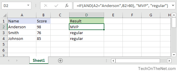
Based on the spreadsheet above, you can combine the IF function with the AND function as follows:

=IF(AND(A2="Anderson",B2>80), "MVP", "regular")
Result: "MVP"

=IF(AND(B2>=80,B2<=100), "Great Score", "Not Bad")
Result: "Great Score"

=IF(AND(B3>=80,B3<=100), "Great Score", "Not Bad")
Result: "Not Bad"

=IF(AND(A2="Anderson",A3="Smith",A4="Johnson"), 100, 50)
Result: 100

=IF(AND(A2="Anderson",A3="Smith",A4="Parker"), 100, 50)
Result: 50

In the examples above, all conditions within the AND function must be TRUE for the condition to be met.

Источник

Examples

Using AND, OR and NOT with Conditional Formatting

Need more help?

See also

Examples of using formulas with IF, AND, OR functions in Excel

Formula with IF and AVERAGE functions for selecting of values by conditions

Formula with logical functions AND IF OR in excel

Features of using logical functions IF, AND, OR in Excel

Что возвращает функция

Синтаксис

Аргументы функции

Дополнительная информация

Функция Если в Excel примеры с несколькими условиями

Пример 1. Проверяем простое числовое условие с помощью функции IF (ЕСЛИ)

Пример 2. Использование вложенной функции IF (ЕСЛИ) для проверки условия выражения

Пример 3. Вычисляем сумму комиссии с продаж с помощью функции IF (ЕСЛИ) в Excel

Пример 4. Используем логические операторы (AND/OR) (И/ИЛИ) в функции IF (ЕСЛИ) в Excel

Пример 5. Преобразуем ошибки в значения “0” с помощью функции IF (ЕСЛИ)

What is a Logical Function?

IF Function example

Excel Logic functions explained

Practical example

Summary

1. AND Function

Syntax

Arguments

Notes

Example

2. FALSE Function

Syntax

Arguments

Notes

Example

3. IF Function

Syntax

Arguments

Notes

Example

4. IFERROR Function

Syntax

Arguments

Notes

Example

5. IFNA Function

Syntax

Arguments

Notes

Example

6. NOT Function

Syntax

Arguments

Notes

Example

7. OR Function

Syntax

Arguments

Notes

Example

8. TRUE Function

Syntax

Arguments

Notes

Example

What is IF Function in Excel?

Table of contents

Syntax of the IF Excel Function

How to Use IF Function in Excel?

Example #1

Example #2

Example #3

Example #4

Example #5

Guidelines for the Multiple IF Statements

Frequently Asked Question

IF Excel Function Video

Recommended Articles

IF Formula Builder

AND Function

OR Function

IF AND Formula