
Excel for Microsoft 365 Excel for Microsoft 365 for Mac Excel for the web Excel 2021 Excel 2021 for Mac Excel 2019 Excel 2019 for Mac Excel 2016 Excel 2016 for Mac Excel 2013 Excel 2010 Excel 2007 Excel for Mac 2011 Excel Starter 2010 More…Less
Use the AND function, one of the logical functions, to determine if all conditions in a test are TRUE.
Example
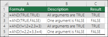
The AND function returns TRUE if all its arguments evaluate to TRUE, and returns FALSE if one or more arguments evaluate to FALSE.
One common use for the AND function is to expand the usefulness of other functions that perform logical tests. For example, the IF function performs a logical test and then returns one value if the test evaluates to TRUE and another value if the test evaluates to FALSE. By using the AND function as the logical_test argument of the IF function, you can test many different conditions instead of just one.
Syntax
AND(logical1, [logical2], …)
The AND function syntax has the following arguments:
|
Argument |
Description |
|---|---|
|
Logical1 |
Required. The first condition that you want to test that can evaluate to either TRUE or FALSE. |
|
Logical2, … |
Optional. Additional conditions that you want to test that can evaluate to either TRUE or FALSE, up to a maximum of 255 conditions. |
Remarks
-
The arguments must evaluate to logical values, such as TRUE or FALSE, or the arguments must be arrays or references that contain logical values.
-
If an array or reference argument contains text or empty cells, those values are ignored.
-
If the specified range contains no logical values, the AND function returns the #VALUE! error.
Examples
Here are some general examples of using AND by itself, and in conjunction with the IF function.
|
Formula |
Description |
|---|---|
|
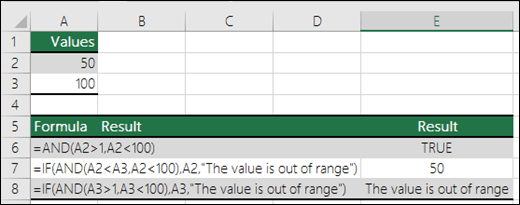
=AND(A2>1,A2<100) |
Displays TRUE if A2 is greater than 1 AND less than 100, otherwise it displays FALSE. |
|
=IF(AND(A2<A3,A2<100),A2,»The value is out of range») |
Displays the value in cell A2 if it’s less than A3 AND less than 100, otherwise it displays the message «The value is out of range». |
|
=IF(AND(A3>1,A3<100),A3,»The value is out of range») |
Displays the value in cell A3 if it is greater than 1 AND less than 100, otherwise it displays a message. You can substitute any message of your choice. |
Bonus Calculation
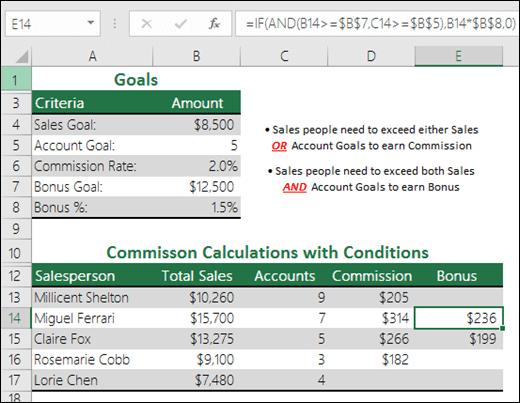
Here is a fairly common scenario where we need to calculate if sales people qualify for a bonus using IF and AND.
-
=IF(AND(B14>=$B$7,C14>=$B$5),B14*$B$8,0) – IF Total Sales are greater than or equal (>=) to the Sales Goal, AND Accounts are greater than or equal to (>=) the Account Goal, then multiply Total Sales by the Bonus %, otherwise return 0.
Need more help?
You can always ask an expert in the Excel Tech Community or get support in the Answers community.
Related Topics
Video: Advanced IF functions
Learn how to use nested functions in a formula
IF function
OR function
NOT function
Overview of formulas in Excel
How to avoid broken formulas
Detect errors in formulas
Keyboard shortcuts in Excel
Logical functions (reference)
Excel functions (alphabetical)
Excel functions (by category)
Need more help?
Purpose
Test multiple conditions with AND
Return value
TRUE if all arguments evaluate TRUE; FALSE if not
Usage notes
The AND function is used to check more than one logical condition at the same time, up to 255 conditions, supplied as arguments. Each argument (logical1, logical2, etc.) must be an expression that returns TRUE or FALSE or a value that can be evaluated as TRUE or FALSE. The arguments provided to the AND function can be constants, cell references, arrays, or logical expressions.
The purpose of the AND function is to evaluate more than one logical test at the same time and return TRUE only if all results are TRUE. For example, if A1 contains the number 50, then:
=AND(A1>0,A1>10,A1<100) // returns TRUE
=AND(A1>0,A1>10,A1<30) // returns FALSE
The AND function will evaluate all values supplied and return TRUE only if all values evaluate to TRUE. If any value evaluates to FALSE, the AND function will return FALSE. Note: Excel will evaluate any number except zero (0) as TRUE.
Both the AND function and the OR function will aggregate results to a single value. This means they can’t be used in array operations that need to deliver an array of results. To work around this limitation, you can use Boolean logic. For more information, see: Array formulas with AND and OR logic.
Examples
To test if the value in A1 is greater than 0 and less than 5, you can use AND like this:
=AND(A1>0,A1<5)
You can embed the AND function inside the IF function. Using the above example, you can supply AND as the logical_test for the IF function like so:
=IF(AND(A1>0,A1<5), "Approved", "Denied")
This formula will return «Approved» only if the value in A1 is greater than 0 and less than 5.
You can combine the AND function with the OR function. The formula below returns TRUE when A1 > 100 and B1 is «complete» or «pending»:
=AND(A1>100,OR(B1="complete",B1="pending"))
See below for many more examples of how the AND function can be used.
Notes
- The AND function is not case-sensitive.
- The AND function does not support wildcards.
- Text values or empty cells supplied as arguments are ignored.
- The AND function will return #VALUE if no logical values are found or created during evaluation.
Содержание
- AND function
- Example
- Examples
- Need more help?
- Overview of formulas in Excel
- Create a formula that refers to values in other cells
- See a formula
- Enter a formula that contains a built-in function
- Download our Formulas tutorial workbook
- Formulas in-depth
- Need more help?
- Using logical functions in Excel: AND, OR, XOR and NOT
- Excel logical functions — overview
- Excel logical functions — facts and figures
- Using the AND function in Excel
- Excel AND function — common uses
- An Excel formula for the BETWEEN condition
- Using the OR function in Excel
- Using the XOR function in Excel
- Using the NOT function in Excel
AND function
Use the AND function, one of the logical functions, to determine if all conditions in a test are TRUE.
Example
The AND function returns TRUE if all its arguments evaluate to TRUE, and returns FALSE if one or more arguments evaluate to FALSE.
One common use for the AND function is to expand the usefulness of other functions that perform logical tests. For example, the IF function performs a logical test and then returns one value if the test evaluates to TRUE and another value if the test evaluates to FALSE. By using the AND function as the logical_test argument of the IF function, you can test many different conditions instead of just one.
The AND function syntax has the following arguments:
Required. The first condition that you want to test that can evaluate to either TRUE or FALSE.
Optional. Additional conditions that you want to test that can evaluate to either TRUE or FALSE, up to a maximum of 255 conditions.
The arguments must evaluate to logical values, such as TRUE or FALSE, or the arguments must be arrays or references that contain logical values.
If an array or reference argument contains text or empty cells, those values are ignored.
If the specified range contains no logical values, the AND function returns the #VALUE! error.
Examples
Here are some general examples of using AND by itself, and in conjunction with the IF function.
=AND(A2>1,A2 AND less than 100, otherwise it displays FALSE.
Displays the value in cell A2 if it’s less than A3 AND less than 100, otherwise it displays the message «The value is out of range».
=IF(AND(A3>1,A3 AND less than 100, otherwise it displays a message. You can substitute any message of your choice.
Here is a fairly common scenario where we need to calculate if sales people qualify for a bonus using IF and AND.
=$B$7,C14>=$B$5),B14*$B$8,0)» loading=»lazy»>
=IF(AND(B14>=$B$7,C14>=$B$5),B14*$B$8,0) – IF Total Sales are greater than or equal (>=) to the Sales Goal, AND Accounts are greater than or equal to (>=) the Account Goal, then multiply Total Sales by the Bonus %, otherwise return 0.
Need more help?
You can always ask an expert in the Excel Tech Community or get support in the Answers community.
Источник
Overview of formulas in Excel
Get started on how to create formulas and use built-in functions to perform calculations and solve problems.

Important: The calculated results of formulas and some Excel worksheet functions may differ slightly between a Windows PC using x86 or x86-64 architecture and a Windows RT PC using ARM architecture. Learn more about the differences.
Important: In this article we discuss XLOOKUP and VLOOKUP, which are similar. Try using the new XLOOKUP function, an improved version of VLOOKUP that works in any direction and returns exact matches by default, making it easier and more convenient to use than its predecessor.
Create a formula that refers to values in other cells
Type the equal sign =.
Note: Formulas in Excel always begin with the equal sign.
Select a cell or type its address in the selected cell.

Enter an operator. For example, – for subtraction.
Select the next cell, or type its address in the selected cell.

Press Enter. The result of the calculation appears in the cell with the formula.
See a formula
When a formula is entered into a cell, it also appears in the Formula bar.

To see a formula, select a cell, and it will appear in the formula bar.

Enter a formula that contains a built-in function
Select an empty cell.
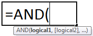
Type an equal sign = and then type a function. For example, =SUM for getting the total sales.
Type an opening parenthesis (.
Select the range of cells, and then type a closing parenthesis).

Press Enter to get the result.
Download our Formulas tutorial workbook
We’ve put together a Get started with Formulas workbook that you can download. If you’re new to Excel, or even if you have some experience with it, you can walk through Excel’s most common formulas in this tour. With real-world examples and helpful visuals, you’ll be able to Sum, Count, Average, and Vlookup like a pro.
Formulas in-depth
You can browse through the individual sections below to learn more about specific formula elements.
A formula can also contain any or all of the following: functions, references, operators, and constants.
Parts of a formula

1. Functions: The PI() function returns the value of pi: 3.142.
2. References: A2 returns the value in cell A2.
3. Constants: Numbers or text values entered directly into a formula, such as 2.
4. Operators: The ^ (caret) operator raises a number to a power, and the * (asterisk) operator multiplies numbers.
A constant is a value that is not calculated; it always stays the same. For example, the date 10/9/2008, the number 210, and the text «Quarterly Earnings» are all constants. An expression or a value resulting from an expression is not a constant. If you use constants in a formula instead of references to cells (for example, =30+70+110), the result changes only if you modify the formula. In general, it’s best to place constants in individual cells where they can be easily changed if needed, then reference those cells in formulas.
A reference identifies a cell or a range of cells on a worksheet, and tells Excel where to look for the values or data you want to use in a formula. You can use references to use data contained in different parts of a worksheet in one formula or use the value from one cell in several formulas. You can also refer to cells on other sheets in the same workbook, and to other workbooks. References to cells in other workbooks are called links or external references.
The A1 reference style
By default, Excel uses the A1 reference style, which refers to columns with letters (A through XFD, for a total of 16,384 columns) and refers to rows with numbers (1 through 1,048,576). These letters and numbers are called row and column headings. To refer to a cell, enter the column letter followed by the row number. For example, B2 refers to the cell at the intersection of column B and row 2.
The cell in column A and row 10
The range of cells in column A and rows 10 through 20
The range of cells in row 15 and columns B through E
All cells in row 5
All cells in rows 5 through 10
All cells in column H
All cells in columns H through J
The range of cells in columns A through E and rows 10 through 20
Making a reference to a cell or a range of cells on another worksheet in the same workbook
In the following example, the AVERAGE function calculates the average value for the range B1:B10 on the worksheet named Marketing in the same workbook.

1. Refers to the worksheet named Marketing
2. Refers to the range of cells from B1 to B10
3. The exclamation point (!) Separates the worksheet reference from the cell range reference
Note: If the referenced worksheet has spaces or numbers in it, then you need to add apostrophes (‘) before and after the worksheet name, like =’123′!A1 or =’January Revenue’!A1.
The difference between absolute, relative and mixed references
Relative references A relative cell reference in a formula, such as A1, is based on the relative position of the cell that contains the formula and the cell the reference refers to. If the position of the cell that contains the formula changes, the reference is changed. If you copy or fill the formula across rows or down columns, the reference automatically adjusts. By default, new formulas use relative references. For example, if you copy or fill a relative reference in cell B2 to cell B3, it automatically adjusts from =A1 to =A2.
Copied formula with relative reference

Absolute references An absolute cell reference in a formula, such as $A$1, always refer to a cell in a specific location. If the position of the cell that contains the formula changes, the absolute reference remains the same. If you copy or fill the formula across rows or down columns, the absolute reference does not adjust. By default, new formulas use relative references, so you may need to switch them to absolute references. For example, if you copy or fill an absolute reference in cell B2 to cell B3, it stays the same in both cells: =$A$1.
Copied formula with absolute reference

Mixed references A mixed reference has either an absolute column and relative row, or absolute row and relative column. An absolute column reference takes the form $A1, $B1, and so on. An absolute row reference takes the form A$1, B$1, and so on. If the position of the cell that contains the formula changes, the relative reference is changed, and the absolute reference does not change. If you copy or fill the formula across rows or down columns, the relative reference automatically adjusts, and the absolute reference does not adjust. For example, if you copy or fill a mixed reference from cell A2 to B3, it adjusts from =A$1 to =B$1.
Copied formula with mixed reference

The 3-D reference style
Conveniently referencing multiple worksheets If you want to analyze data in the same cell or range of cells on multiple worksheets within a workbook, use a 3-D reference. A 3-D reference includes the cell or range reference, preceded by a range of worksheet names. Excel uses any worksheets stored between the starting and ending names of the reference. For example, =SUM(Sheet2:Sheet13!B5) adds all the values contained in cell B5 on all the worksheets between and including Sheet 2 and Sheet 13.
You can use 3-D references to refer to cells on other sheets, to define names, and to create formulas by using the following functions: SUM, AVERAGE, AVERAGEA, COUNT, COUNTA, MAX, MAXA, MIN, MINA, PRODUCT, STDEV.P, STDEV.S, STDEVA, STDEVPA, VAR.P, VAR.S, VARA, and VARPA.
3-D references cannot be used in array formulas.
3-D references cannot be used with the intersection operator (a single space) or in formulas that use implicit intersection.
What occurs when you move, copy, insert, or delete worksheets The following examples explain what happens when you move, copy, insert, or delete worksheets that are included in a 3-D reference. The examples use the formula =SUM(Sheet2:Sheet6!A2:A5) to add cells A2 through A5 on worksheets 2 through 6.
Insert or copy If you insert or copy sheets between Sheet2 and Sheet6 (the endpoints in this example), Excel includes all values in cells A2 through A5 from the added sheets in the calculations.
Delete If you delete sheets between Sheet2 and Sheet6, Excel removes their values from the calculation.
Move If you move sheets from between Sheet2 and Sheet6 to a location outside the referenced sheet range, Excel removes their values from the calculation.
Move an endpoint If you move Sheet2 or Sheet6 to another location in the same workbook, Excel adjusts the calculation to accommodate the new range of sheets between them.
Delete an endpoint If you delete Sheet2 or Sheet6, Excel adjusts the calculation to accommodate the range of sheets between them.
The R1C1 reference style
You can also use a reference style where both the rows and the columns on the worksheet are numbered. The R1C1 reference style is useful for computing row and column positions in macros. In the R1C1 style, Excel indicates the location of a cell with an «R» followed by a row number and a «C» followed by a column number.
A relative reference to the cell two rows up and in the same column
A relative reference to the cell two rows down and two columns to the right
An absolute reference to the cell in the second row and in the second column
A relative reference to the entire row above the active cell
An absolute reference to the current row
When you record a macro, Excel records some commands by using the R1C1 reference style. For example, if you record a command, such as clicking the AutoSum button to insert a formula that adds a range of cells, Excel records the formula by using R1C1 style, not A1 style, references.
You can turn the R1C1 reference style on or off by setting or clearing the R1C1 reference style check box under the Working with formulas section in the Formulas category of the Options dialog box. To display this dialog box, click the File tab.
Need more help?
You can always ask an expert in the Excel Tech Community or get support in the Answers community.
Источник
Using logical functions in Excel: AND, OR, XOR and NOT
 by Svetlana Cheusheva, updated on October 7, 2022
The tutorial explains the essence of Excel logical functions AND, OR, XOR and NOT and provides formula examples that demonstrate their common and inventive uses.
Last week we tapped into the insight of Excel logical operators that are used to compare data in different cells. Today, you will see how to extend the use of logical operators and construct more elaborate tests to perform more complex calculations. Excel logical functions such as AND, OR, XOR and NOT will help you in doing this.
Excel logical functions — overview
Microsoft Excel provides 4 logical functions to work with the logical values. The functions are AND, OR, XOR and NOT. You use these functions when you want to carry out more than one comparison in your formula or test multiple conditions instead of just one. As well as logical operators, Excel logical functions return either TRUE or FALSE when their arguments are evaluated.
The following table provides a short summary of what each logical function does to help you choose the right formula for a specific task.
| Function | Description | Formula Example | Formula Description |
| AND | Returns TRUE if all of the arguments evaluate to TRUE. | =AND(A2>=10, B2 | The formula returns TRUE if a value in cell A2 is greater than or equal to 10, and a value in B2 is less than 5, FALSE otherwise. |
| OR | Returns TRUE if any argument evaluates to TRUE. | =OR(A2>=10, B2 | The formula returns TRUE if A2 is greater than or equal to 10 or B2 is less than 5, or both conditions are met. If neither of the conditions it met, the formula returns FALSE. |
| XOR | Returns a logical Exclusive Or of all arguments. | =XOR(A2>=10, B2 | The formula returns TRUE if either A2 is greater than or equal to 10 or B2 is less than 5. If neither of the conditions is met or both conditions are met, the formula returns FALSE. |
| NOT | Returns the reversed logical value of its argument. I.e. If the argument is FALSE, then TRUE is returned and vice versa. | =NOT(A2>=10) | The formula returns FALSE if a value in cell A1 is greater than or equal to 10; TRUE otherwise. |
In additions to the four logical functions outlined above, Microsoft Excel provides 3 «conditional» functions — IF, IFERROR and IFNA.
Excel logical functions — facts and figures
- In arguments of the logical functions, you can use cell references, numeric and text values, Boolean values, comparison operators, and other Excel functions. However, all arguments must evaluate to the Boolean values of TRUE or FALSE, or references or arrays containing logical values.
- If an argument of a logical function contains any empty cells, such values are ignored. If all of the arguments are empty cells, the formula returns #VALUE! error.
- If an argument of a logical function contains numbers, then zero evaluates to FALSE, and all other numbers including negative numbers evaluate to TRUE. For example, if cells A1:A5 contain numbers, the formula =AND(A1:A5) will return TRUE if none of the cells contains 0, FALSE otherwise.
- A logical function returns the #VALUE! error if none of the arguments evaluate to logical values.
- A logical function returns the #NAME? error if you’ve misspell the function’s name or attempted to use the function in an earlier Excel version that does not support it. For example, the XOR function can be used in Excel 2016 and 2013 only.
- In Excel 2007 and higher, you can include up to 255 arguments in a logical function, provided that the total length of the formula does not exceed 8,192 characters. In Excel 2003 and lower, you can supply up to 30 arguments and the total length of your formula shall not exceed 1,024 characters.
Using the AND function in Excel
The AND function is the most popular member of the logic functions family. It comes in handy when you have to test several conditions and make sure that all of them are met. Technically, the AND function tests the conditions you specify and returns TRUE if all of the conditions evaluate to TRUE, FALSE otherwise.
The syntax for the Excel AND function is as follows:
Where logical is the condition you want to test that can evaluate to either TRUE or FALSE. The first condition (logical1) is required, subsequent conditions are optional.
And now, let’s look at some formula examples that demonstrate how to use the AND functions in Excel formulas.
| Formula | Description |
| =AND(A2=»Bananas», B2>C2) | Returns TRUE if A2 contains «Bananas» and B2 is greater than C2, FALSE otherwise. |
| =AND(B2>20, B2=C2) | Returns TRUE if B2 is greater than 20 and B2 is equal to C2, FALSE otherwise. |
| =AND(A2=»Bananas», B2>=30, B2>C2) | Returns TRUE if A2 contains «Bananas», B2 is greater than or equal to 30 and B2 is greater than C2, FALSE otherwise. |

Excel AND function — common uses
By itself, the Excel AND function is not very exciting and has narrow usefulness. But in combination with other Excel functions, AND can significantly extend the capabilities of your worksheets.
One of the most common uses of the Excel AND function is found in the logical_test argument of the IF function to test several conditions instead of just one. For example, you can nest any of the AND functions above inside the IF function and get a result similar to this:
=IF(AND(A2=»Bananas», B2>C2), «Good», «Bad») 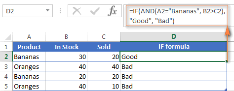
For more IF / AND formula examples, please check out his tutorial: Excel IF function with multiple AND conditions.
An Excel formula for the BETWEEN condition
If you need to create a between formula in Excel that picks all values between the given two values, a common approach is to use the IF function with AND in the logical test.
For example, you have 3 values in columns A, B and C and you want to know if a value in column A falls between B and C values. To make such a formula, all it takes is the IF function with nested AND and a couple of comparison operators:
Formula to check if X is between Y and Z, inclusive:
Formula to check if X is between Y and Z, not inclusive:
=IF(AND(A2>B2, A2 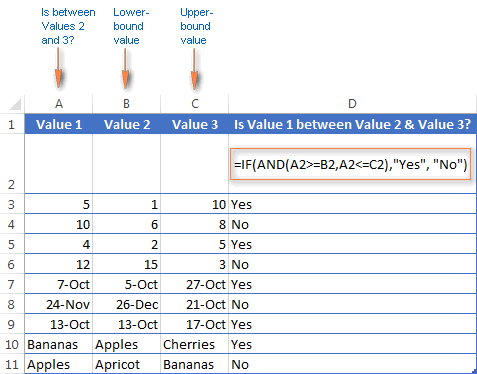
As demonstrated in the screenshot above, the formula works perfectly for all data types — numbers, dates and text values. When comparing text values, the formula checks them character-by-character in the alphabetic order. For example, it states that Apples in not between Apricot and Bananas because the second «p» in Apples comes before «r» in Apricot. Please see Using Excel comparison operators with text values for more details.
As you see, the IF /AND formula is simple, fast and almost universal. I say «almost» because it does not cover one scenario. The above formula implies that a value in column B is smaller than in column C, i.e. column B always contains the lower bound value and C — the upper bound value. This is the reason why the formula returns «No» for row 6, where A6 has 12, B6 — 15 and C6 — 3 as well as for row 8 where A8 is 24-Nov, B8 is 26-Dec and C8 is 21-Oct.
But what if you want your between formula to work correctly regardless of where the lower-bound and upper-bound values reside? In this case, use the Excel MEDIAN function that returns the median of the given numbers (i.e. the number in the middle of a set of numbers).
So, if you replace AND in the logical test of the IF function with MEDIAN, the formula will go like:
And you will get the following results: 
As you see, the MEDIAN function works perfectly for numbers and dates, but returns the #NUM! error for text values. Alas, no one is perfect : )
If you want a perfect Between formula that works for text values as well as for numbers and dates, then you will have to construct a more complex logical text using the AND / OR functions, like this:
=IF(OR(AND(A2>B2, A2 C2)), «Yes», «No») 
Using the OR function in Excel
As well as AND, the Excel OR function is a basic logical function that is used to compare two values or statements. The difference is that the OR function returns TRUE if at least one if the arguments evaluates to TRUE, and returns FALSE if all arguments are FALSE. The OR function is available in all versions of Excel 2016 — 2000.
The syntax of the Excel OR function is very similar to AND:
Where logical is something you want to test that can be either TRUE or FALSE. The first logical is required, additional conditions (up to 255 in modern Excel versions) are optional.
And now, let’s write down a few formulas for you to get a feel how the OR function in Excel works.
| Formula | Description |
| =OR(A2=»Bananas», A2=»Oranges») | Returns TRUE if A2 contains «Bananas» or «Oranges», FALSE otherwise. |
| =OR(B2>=40, C2>=20) | Returns TRUE if B2 is greater than or equal to 40 or C2 is greater than or equal to 20, FALSE otherwise. |
| =OR(B2=» «, C2=»») | Returns TRUE if either B2 or C2 is blank or both, FALSE otherwise. |

As well as Excel AND function, OR is widely used to expand the usefulness of other Excel functions that perform logical tests, e.g. the IF function. Here are just a couple of examples:
IF function with nested OR
=IF(OR(B2>30, C2>20), «Good», «Bad»)
The formula returns «Good» if a number in cell B3 is greater than 30 or the number in C2 is greater than 20, «Bad» otherwise.
Excel AND / OR functions in one formula
Naturally, nothing prevents you from using both functions, AND & OR, in a single formula if your business logic requires this. There can be infinite variations of such formulas that boil down to the following basic patterns:
=AND(OR(Cond1, Cond2), Cond3)
=AND(OR(Cond1, Cond2), OR(Cond3, Cond4)
=OR(AND(Cond1, Cond2), Cond3)
For example, if you wanted to know what consignments of bananas and oranges are sold out, i.e. «In stock» number (column B) is equal to the «Sold» number (column C), the following OR/AND formula could quickly show this to you:
=OR(AND(A2=»bananas», B2=C2), AND(A2=»oranges», B2=C2)) 
OR function in Excel conditional formatting
The rule with the above OR formula highlights rows that contain an empty cell either in column B or C, or in both. 
For more information about conditional formatting formulas, please see the following articles:
Using the XOR function in Excel
In Excel 2013, Microsoft introduced the XOR function, which is a logical Exclusive OR function. This term is definitely familiar to those of you who have some knowledge of any programming language or computer science in general. For those who don’t, the concept of ‘Exclusive Or’ may be a bit difficult to grasp at first, but hopefully the below explanation illustrated with formula examples will help.
The syntax of the XOR function is identical to OR’s :
The first logical statement (Logical 1) is required, additional logical values are optional. You can test up to 254 conditions in one formula, and these can be logical values, arrays, or references that evaluate to either TRUE or FALSE.
In the simplest version, an XOR formula contains just 2 logical statements and returns:
- TRUE if either argument evaluates to TRUE.
- FALSE if both arguments are TRUE or neither is TRUE.
This might be easier to understand from the formula examples:
| Formula | Result | Description |
| =XOR(1>0, 2 | TRUE | Returns TRUE because the 1st argument is TRUE and the 2 nd argument is FALSE. |
| =XOR(1 | FALSE | Returns FALSE because both arguments are FALSE. |
| =XOR(1>0, 2>1) | FALSE | Returns FALSE because both arguments are TRUE. |
When more logical statements are added, the XOR function in Excel results in:
- TRUE if an odd number of the arguments evaluate to TRUE;
- FALSE if is the total number of TRUE statements is even, or if all statements are FALSE.
The screenshot below illustrates the point: 
If you are not sure how the Excel XOR function can be applied to a real-life scenario, consider the following example. Suppose you have a table of contestants and their results for the first 2 games. You want to know which of the payers shall play the 3 rd game based on the following conditions:
- Contestants who won Game 1 and Game 2 advance to the next round automatically and don’t have to play Game 3.
- Contestants who lost both first games are knocked out and don’t play Game 3 either.
- Contestants who won either Game 1 or Game 2 shall play Game 3 to determine who goes into the next round and who doesn’t.
A simple XOR formula works exactly as we want:
=XOR(B2=»Won», C2=»Won») 
And if you nest this XOR function into the logical test of the IF formula, you will get even more sensible results:
=IF(XOR(B2=»Won», C2=»Won»), «Yes», «No») 
Using the NOT function in Excel
The NOT function is one of the simplest Excel functions in terms of syntax:
You use the NOT function in Excel to reverse a value of its argument. In other words, if logical evaluates to FALSE, the NOT function returns TRUE and vice versa. For example, both of the below formulas return FALSE:
Why would one want to get such ridiculous results? In some cases, you might be more interested to know when a certain condition isn’t met than when it is. For example, when reviewing a list of attire, you may want to exclude some color that does not suit you. I’m not particularly fond of black, so I go ahead with this formula:
=NOT(C2=»black») 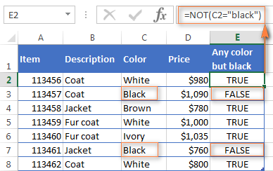
As usual, in Microsoft Excel there is more than one way to do something, and you can achieve the same result by using the Not equal to operator: =C2<>«black».
If you want to test several conditions in a single formula, you can use NOT in conjunctions with the AND or OR function. For example, if you wanted to exclude black and white colors, the formula would go like:
And if you’d rather not have a black coat, while a black jacket or a back fur coat may be considered, you should use NOT in combination with the Excel AND function:
Another common use of the NOT function in Excel is to reverse the behavior of some other function. For instance, you can combine NOT and ISBLANK functions to create the ISNOTBLANK formula that Microsoft Excel lacks.
As you know, the formula =ISBLANK(A2) returns TRUE of if the cell A2 is blank. The NOT function can reverse this result to FALSE: =NOT(ISBLANK(A2))
And then, you can take a step further and create a nested IF statement with the NOT / ISBLANK functions for a real-life task:
=IF(NOT(ISBLANK(C2)), C2*0.15, «No bonus :(«) ![]()
Translated into plain English, the formula tells Excel to do the following. If the cell C2 is not empty, multiply the number in C2 by 0.15, which gives the 15% bonus to each salesman who has made any extra sales. If C2 is blank, the text «No bonus :(» appears.
In essence, this is how you use the logical functions in Excel. Of course, these examples have only scratched the surface of AND, OR, XOR and NOT capabilities. Knowing the basics, you can now extend your knowledge by tackling your real tasks and writing smart elaborate formulas for your worksheets.
Источник
На чтение 2 мин
Функция AND (И) в Excel используется для сравнения нескольких условий.
Содержание
- Что возвращает функция
- Синтаксис
- Аргументы функции
- Дополнительная информация
- Примеры использования функции AND (И, ИЛИ) в Excel
Что возвращает функция
Возвращает TRUE если значение или условие, при сравнении, соответствует критериям заданным в функции, или FALSE, в случае, если условие не соответствует критериям.
Синтаксис
=AND(logical1, [logical2],…) — английская версия
=И(логическое_значение1;[логическое_значение2];…) — русская версия
Аргументы функции
- logical1 (логическое_значение1) — первое условие, которое вы хотите оценить с помощью функции;
- [logical2] ([логическое_значение2]) (не обязательно) — второе условие, которое вы хотите оценить с помощью функции.
Дополнительная информация
- Функция может быть использована совместно с другими формулами;
- Например, с помощью функции IF (ЕСЛИ) вы можете проверить условие, а затем указать значение, когда оно TRUE, и значение, когда оно равно FALSE. Использование функции AND (И) вместе с функцией IF (ЕСЛИ) позволяет тестировать несколько условий за один раз;
Например, если вы хотите проверить значение в ячейке A1 на предмет того, больше оно чем «0» или меньше чем «100», то вы можете использовать следующую формулу:
=IF(AND(A1>0,A1<100),”Approve”,”Reject”) — английская версия
Больше лайфхаков в нашем Telegram Подписаться
=ЕСЛИ(И(A1>0;A1<100);»Одобрить»;»Против») — русская версия
- Аргументы функции должны быть логически вычислимы по принципу (TRUE/FALSE);
- Ячейки с пустыми или текстовыми значениями игнорируются функцией;
- Если в качестве аргументов функции не указаны логически вычислимые данные, то функция выдаст ошибку #VALUE!;
- Одновременно вы можете тестировать до 255 условий в рамках одного использования функции.
Примеры использования функции AND (И, ИЛИ) в Excel

The AND Function in excel is a logical function that tests multiple conditions and returns “true” or “false” depending on whether they are met or not. The formula of AND function is “=AND(logical1,[logical2]…),” where “logical1” is the first condition to evaluate.
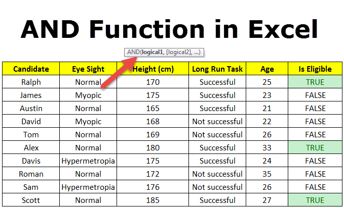
Table of contents
- AND Function in Excel
- Syntax of the AND Function
- The Characteristics of AND Function
- The Output of AND Function
- How to Use AND Function in Excel?
- Example #1–AND Function
- Example #2–AND Function With Nested IF Function
- Example #3–AND Function With Nested IF Function
- Nesting of AND Function in Excel
- Example #4–Nested AND Function
- Limitations of AND Function
- Frequently Asked Questions
- Recommended Articles
Syntax of the AND Function
The syntax is stated as follows:
The function accepts the following arguments:
- Logical 1: This is the first condition or logical value to evaluate.
- Logical 2: This is the second condition or logical value to evaluate.
The “logical 1” is a mandatory argument and “logical 2” is an optional argument.
The Characteristics of AND Function
- It returns “true” if all conditions or logical values evaluate to true.
- It returns “false” if any of the conditions or logical values evaluates to false.
- It can have more logical values depending on the situation and the requirement.
- It treats the value zero as “false” and all non-zero values as “true” while evaluating numbers.
- It ignores empty cells provided as an argument.
- It is often used in combination with other Excel functionsExcel functions help the users to save time and maintain extensive worksheets. There are 100+ excel functions categorized as financial, logical, text, date and time, Lookup & Reference, Math, Statistical and Information functions.read more like IF, OR, and so on.
The Output of AND Function
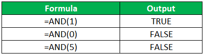
The output in different situations is given as follows:
The output while evaluating numbers is given as follows:
How to Use AND Function in Excel?
It is easy to use the AND function. Let us understand its working with the help of a few examples.
You can download this AND Function Excel Template here – AND Function Excel Template
Example #1–AND Function
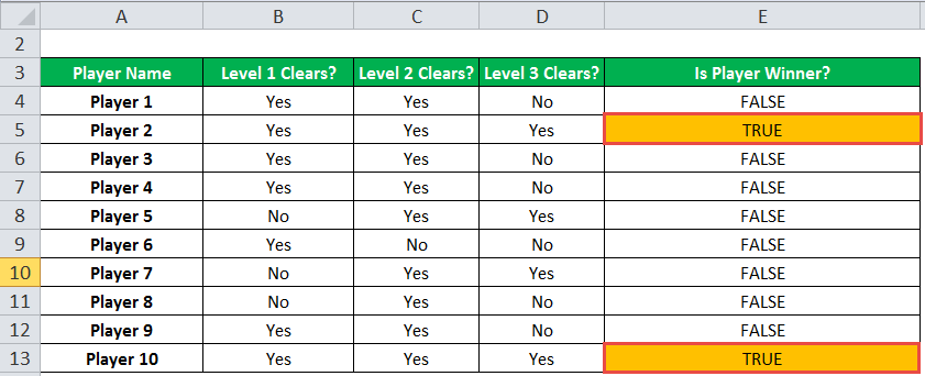
There are three levels and ten players in a game. To be a winner, a player has to clear all three levels. The player loses if he/she fails in any of the three levels.
The performance of the players in different levels is given in the following table. We are required to determine the winner.
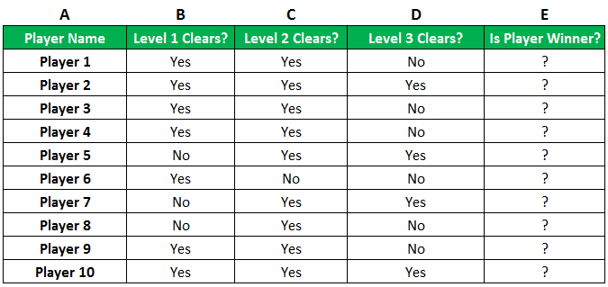
We apply AND formula in column E.
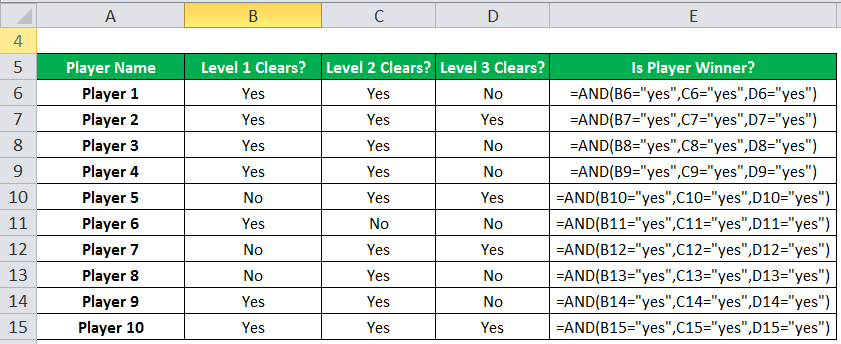
The output of the formula appears in column E.
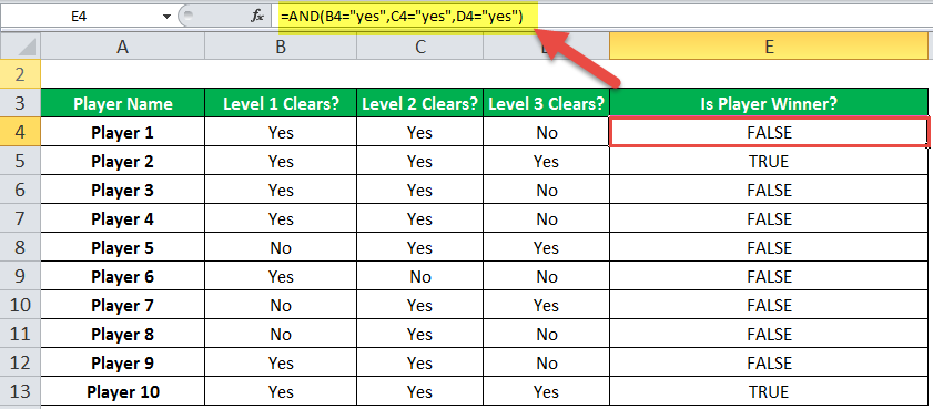
Player 2 and player 10 have cleared all the levels. Since all the logical conditions for these two players are met, the AND function gives the output “true.”
The rest of the players were unable to clear all three levels. If any of the levels is not cleared, the AND function returns “false.”
Example #2–AND Function With Nested IF Function
Let us consider the following example.
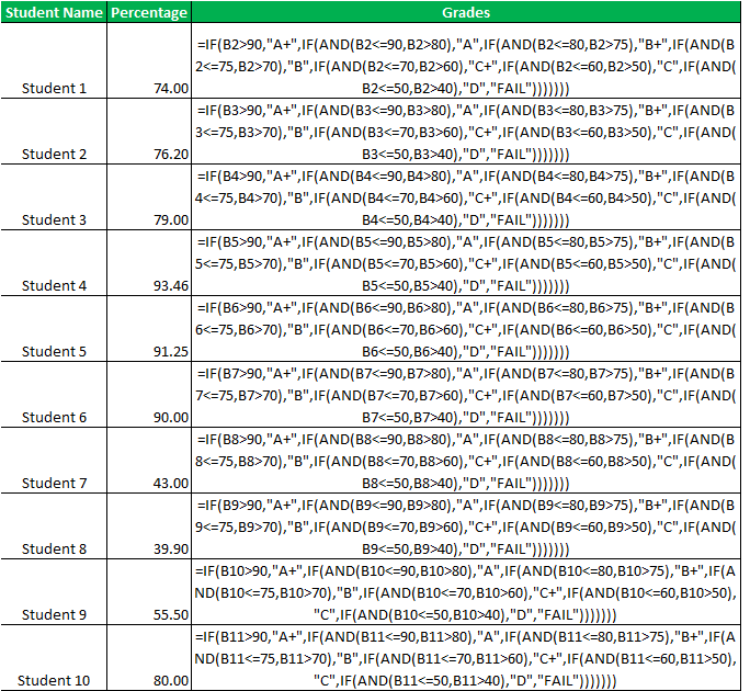
We have the marks (in percentage) of ten students in a school. We have to determine the grade obtained by each student according to the criteria given.
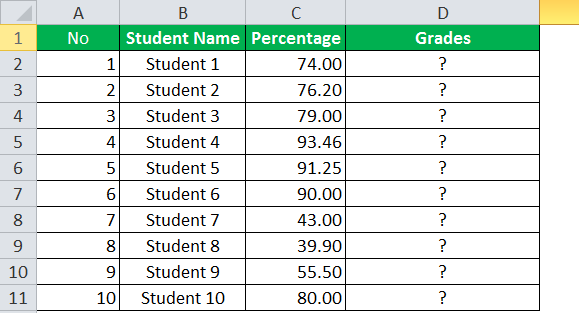
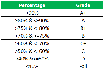
A student obtains “A+” if he/she scores more than 90%. If the percentage is greater than or equal to 80% but less than or equal to 90%, grade “A” is given.
If the percentage is less than 40%, the student fails. Likewise, the grades for the different percentages are given in the following table.
We apply the following formula.
“=IF(B2>90,”A+”,IF(AND(B2<=90,B2>80),”A”,IF(AND(B2<=80,B2>75),”B+”,IF(AND(B2<=75,B2>70),”B”,IF(AND(B2<=70,B2>60),”C+”,IF(AND(B2<=60,B2>50),”C”,IF(AND(B2<=50,B2>40),”D”,”FAIL”)))))))”
We use the nested IF functionIn Excel, nested if function means using another logical or conditional function with the if function to test multiple conditions. For example, if there are two conditions to be tested, we can use the logical functions AND or OR depending on the situation, or we can use the other conditional functions to test even more ifs inside a single if.read more with multiple AND functions to compute the grades. The latter allows testing two conditions together.
The syntax of the IF function is stated as follows:
“=IF(logical_test,[value_if_true],[value_if_false])”
The IF function returns “true” if the condition is met, else returns “false.”
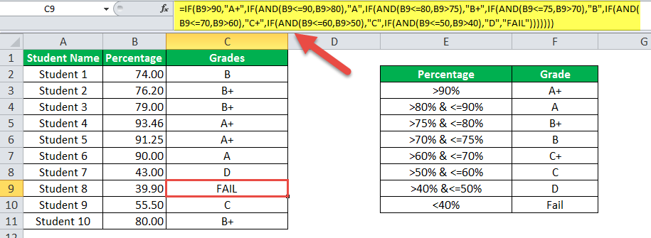
The first logical test is “B2>90.” If this condition is “true,” grade “A+” is assigned. If this condition is “false,” the IF function evaluates the next condition.
The next logical testA logical test in Excel results in an analytical output, either true or false. The equals to operator, “=,” is the most commonly used logical test.read more is “B2<=90, B2>80.” If this condition is “true,” grade “A” is assigned. If this condition is “false,” the next statement is evaluated. Likewise, the IF function tests every condition given in the formula.
The last logical test is “B2<=50, B2>40.” If this condition is “true,” grade “D” is assigned, else the student fails.
We apply the formula to all categories of students, as shown in the following image.
The output of the formula is shown in the succeeding image.
Example #3–AND Function With Nested IF Function
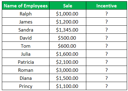
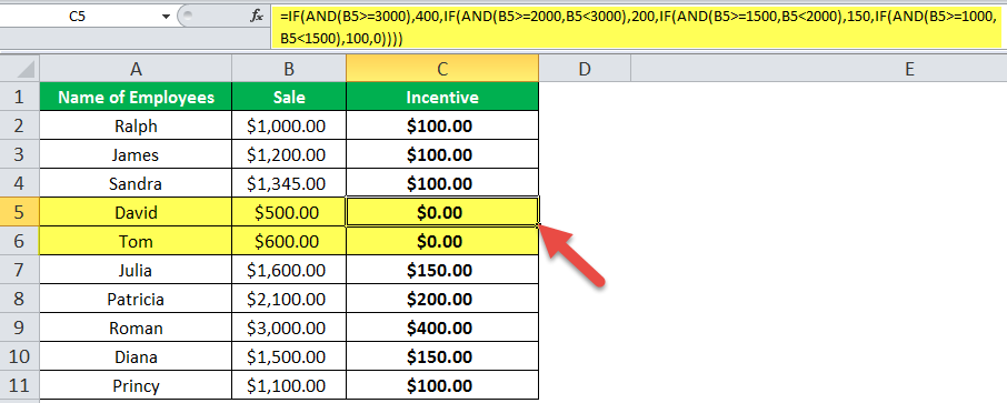
The name of employees and the sales revenueSales revenue refers to the income generated by any business entity by selling its goods or providing its services during the normal course of its operations. It is reported annually, quarterly or monthly as the case may be in the business entity’s income statement/profit & loss account.read more generated by them for an organization are shown in the succeeding image. Every employee is given a monetary incentive depending on the total sales made by him/her.
We have to calculate the incentives of all the employees based on their performance.
The incentive criteria followed by the organization is given in the succeeding table.
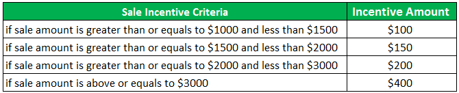
We apply the following formula.
“=IF(AND(B2>=3000),400,IF(AND(B2>=2000,B2<3000),200,IF(AND(B2>=1500,B2<2000),150,IF(AND(B2>=1000,B2<1500),100,0))))”
We use multiple IFs In Excel, multiple IF conditions are IF statements that are contained within another IF statement. They are used to test multiple conditions at the same time and return distinct values. Additional IF statements can be included in the ‘value if true’ and ‘value if false’ arguments of a standard IF formula.read moreand multiple AND functions to calculate the incentives received by all the employees, as shown in the following table.
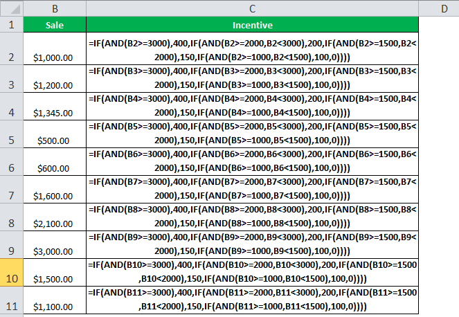
Roman generates sales revenue of $3000. So, he receives an incentive amount of $400.
The revenue generated by David and Tom is $500 and $600, respectively. To be eligible for an incentive, minimum sales of $1000 is required. Hence, they do not get any incentive.
Nesting of AND Function in Excel
A nested function refers to using a function inside another Excel function. In Excel, the nesting of functions up to 64 levels is allowed.
Example #4–Nested AND Function
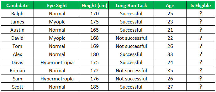
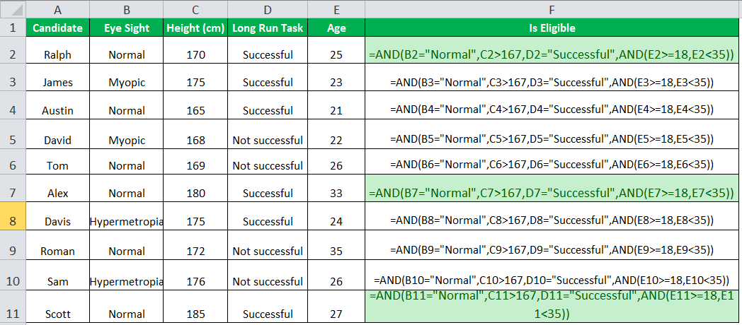
We have a list of candidates who wish to join the Army subject to certain conditions. The eligibility criteria are stated as follows:
- The age should be greater than or equal to 18, but less than 35 years.
- The height should be greater than 167 cm.
- The eyesight should be normal.
- The candidate must have completed the long-run task.
We need to find out the candidates who are eligible for joining the Army.
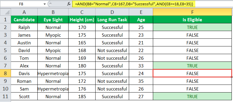
To evaluate the candidates on the given parameters, we use the nested AND function.
We apply the following formula.
“=AND(B2=”Normal”,C2>167,D2=”Successful”,AND(E2>=18,E2<35))”
We evaluate multiple logical conditions simultaneously. We also check whether the age is within the prescribed limit or not. So, we use the AND function inside another AND function.
The output of the formula is shown in the succeeding image.
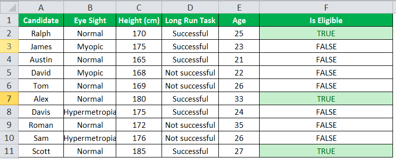
The candidates Ralph, Alex, and Scott pass the selection criteria. Hence, their eligibility output (in column F) is “true.” The remaining candidates are not eligible for joining the Army.
Limitations of AND Function
The limitations are listed as follows:
- With Excel 2007 onwards, the AND function can test up to 255 arguments given that the length of the formula does not exceed 8,162 characters.
- In Excel 2003 and previous versions, the AND function can test up to 30 arguments given that the length of the formula does not exceed 1,024 characters.
- The AND function returns “#VALUE! error#VALUE! Error in Excel represents that the reference cell the user has either entered an incorrect formula or used a wrong data type (mostly numerical data). Sometimes, it is difficult to identify the kind of mistake behind this error.read more” if logical conditions are passed as text or if none of the arguments evaluates to a logical value.
- The AND function returns “#VALUE! error” if all the arguments provided are empty cells.
The following two images show the output of the AND function when an empty cell and a text string is provided as an argument.

Frequently Asked Questions
#1 – When should the AND function of Excel be used
#2 – How is the AND function used with the OR function in Excel?
The OR function helps compare two values or statements. The AND function is combined with the OR function by the following formulas:
“=AND(OR(Condition1,Condition2),Condition3)”
“=AND(OR(Condition1,Condition2),OR(Condition3,Condition4)”
“=OR(AND(Condition1,Condition2),Condition3)”
“=OR(AND(Condition1,Condition2),AND(Condition3,Condition4))”
#3 – What is the difference between AND, IF, and OR functions in Excel?
The difference between the three functions is stated as follows:
– The AND function helps evaluate multiple conditions at the same time. It returns “true” when all conditions are true; otherwise, it returns “false.”
– The IF function helps compare the value with the result expected by the user. It returns specific values for the “true” and “false” outcomes.
– The OR function helps compare two values or two statements. It returns “true” when at least one of the specified conditions is met. It returns “false” if all the logical values evaluate to false.
- The AND function tests multiple conditions and returns “true” or “false” depending upon whether they are met or not.
- The AND function returns “true” if all conditions evaluate to true and returns “false” if any of the conditions evaluates to false.
- The AND function treats the value zero as “false.”
- The AND function can test up to 255 arguments in the latest versions of Excel.
- The AND function returns “#VALUE! error” if logical conditions are passed as a text.
- The formula of the IF function is “=IF(logical_test,[value_if_true],[value_if_false]).”
Recommended Articles
This has been a guide to AND Function in Excel. Here we discuss how to use AND Formula in Excel along with examples and downloadable excel templates. You may also look at these useful functions in Excel –
- Excel Pivot Table Add ColumnThe pivot table add column helps to add a new column in a pivot table.read more
- Excel Convert FunctionAs the word itself, the Excel CONVERT function defines that it can convert the numbers from one measurement system to another measurement system.read more
- VBA Boolean Data TypeBoolean is an inbuilt data type in VBA used for logical references or logical variables. The value this data type holds is either TRUE or FALSE and is used for logical comparison. The declaration of this data type is similar to all the other data types.read more
- IF AND Formula in ExcelThe IF AND excel formula is the combination of two different logical functions often nested together that enables the user to evaluate multiple conditions using AND functions. Based on the output of the AND function, the IF function returns either the “true” or “false” value, respectively.
read more

| Раздел функций | Логические |
| Название на английском | AND |
| Волатильность | Не волатильная |
| Похожие функции | ИЛИ, НЕ, ЕСЛИ |
Что делает эта функция?
Эта функция проверяет два или более условий, чтобы увидеть, все ли они верны.
Её можно использовать для проверки того, что ряд чисел удовлетворяет определенным условиям.
Её можно использовать для проверки того, что число или дата попадают между верхним и нижним пределами.
Как и функция ИЛИ, обычно используется в паре другими логическими функциями, наиболее часто с функцией ЕСЛИ, и с формулами массива
Синтаксис
=И(Выражение1;Выражение2…)
=И(ДиапазонЗначений)
Форматирование
Функция корректно обработает:
- Числа и вычисления, возвращающие их
- Логические выражения (ИСТИНА, ЛОЖЬ) и вычисления, возвращающие их
- Ячейки, содержащие их
- Диапазоны ячеек, если хотя бы одна ячейка содержит числа, ИСТИНА или ЛОЖЬ
- Массивы значений или вычислений
Если на вход подается диапазон, в значениях которого присутствуют текстовые значения, они не учитываются функцией, как и пустые ячейки.
Функция выдаст ошибку, если:
- на вход получены только текстовые или пустые ячейки (одна или несколько)
- среди значений есть ошибки (#ЗНАЧ!, #Н/Д, #ИМЯ?, #ПУСТО!, #ДЕЛ/0!, #ССЫЛКА!, #ЧИСЛО!)
Примеры применения
Пример 1
В следующем примере показан список результатов теста.
Учитель хочет найти учеников, которые набрали выше среднего по всем трем экзаменам.
Функция И использовалась для проверки того, что балл по каждому предмету выше среднего.
Результат ИСТИНА показан для учеников, которые набрали выше среднего во всех трех экзаменах.

Пример 2
Родители выбирают имя для девочки, хотят, чтобы в имени присутствовали мягкие звуки (все три).
Excel не позволяет фильтровать строки по более чем двум критериям.
Но для этой задачи можно воспользоваться формулой массива с функцией И в сочетании с функцией ПОИСК и ЕЧИСЛО.
Обратите внимание, что для того, чтобы функция проверяла вхождения всех букв, это должна быть именно формула массива. Ее нужно вводить без фигурных скобок, но ввод в ячейку осуществлять с помощью сочетания клавиш Ctrl+Shift+Enter.

Файл с примерами
Ниже интерактивный просмотр файла с вышеуказанными примерами. Можно редактировать ячейки, двойной клик по ячейке с формулой поможет просмотреть ее и скопировать.
Другие логические функции
ЕСЛИ, ИЛИ, НЕ
Просмотров 4.3к. Обновлено 17 сентября 2021
Функция И в Excel — это логическая функция, которая требует одновременного выполнения нескольких условий. И возвращает ИСТИНА если все аргументы имеют значение ИСТИНА или ЛОЖЬ если хотябы один из аргументов имеет значение ЛОЖЬ. Чтобы проверить, является ли число в A1 больше нуля и меньше 10, используйте
=И(A1> 0, A1 <10). Функцию И можно использовать в качестве логической проверки внутри функции ЕСЛИ, чтобы избежать дополнительных вложенных ЕСЛИ, и ее можно комбинировать с функцией ИЛИ.
| Функция AND на Русском | Функция И на Английском |
|---|---|
| И | AND |
Содержание
- Синтаксис
- Примеры использования функции И
- Пример 1
- Пример 2
- Пример 3
- Пример 4
Синтаксис
Синтаксис функции И
И (логический1; [логический2]; …)
Функция AND(И) имеет 1 обязательный аргумент и может использоваться для одновременной проверки до 255 условий, передаваемых в качестве аргументов, в Excel 2003 функция может обрабатывать не более 30 аргументов. Каждый аргумент ( логическое_значение1 , логическое_значение2 и т. Д.) Должен быть выражением, возвращающим ИСТИНА или ЛОЖЬ, или значением, которое может быть оценено как ИСТИНА или ЛОЖЬ. Аргументы, предоставляемые функции И, могут быть константами, ссылками на ячейки, массивами или логическими выражениями.
Назначение функции И — оценить более одного логического теста одновременно и вернуть ИСТИНА, только если все результаты ИСТИНА. Например, если B3 содержит число 40, то:
=И(B3 > 10; B3 > 20; B3 < 80) // возвращает ИСТИНА=И(B3 > 10;B3 > 20;B3 < 35) // возвращает ЛОЖЬФункция И будет оценивать все предоставленные значения и возвращать ИСТИНА, только если все значения оцениваются как ИСТИНА. Если какое-либо значение оценивается как ЛОЖЬ, функция И вернет ЛОЖЬ. Примечание. Excel оценит любое число, кроме нуля (0), как ИСТИННОЕ.
Как и функция И функция ИЛИ будет объединять результаты в одном значении. Это означает, что их нельзя использовать в операциях с массивами, которые должны выдавать массив результатов. Чтобы обойти это ограничение, вы можете использовать логическую логику. Для получения дополнительной информации см .: Формулы массивов с логикой И и ИЛИ.
Примечания :
Текстовые значения или пустые ячейки, предоставленные в качестве аргументов, игнорируютсяФункция И возвращает #ЗНАЧ! если во время оценки не найдено или не создано логическое значение
Примеры использования функции И
Пример 1
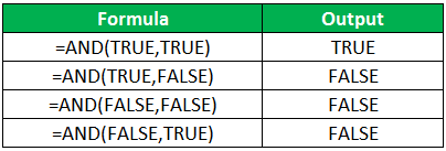
В следующей таблице показаны три примера функции И в Excel:
Обратите внимание, что в приведенном выше примере электронной таблицы:
- функция в ячейке Е2 оценивается как ИСТИНА, поскольку ОБА из поставленных условий ИСТИНА;
- функция в ячейке Е3 оценивается как ЛОЖЬ, поскольку третье условие, С3> 22 , ЛОЖЬ;
- функция в ячейке Е4 оценивается как ЛОЖЬ, поскольку ВСЕ предоставленные условия — ЛОЖЬ.
Пример 2
Чтобы проверить, является ли значение в B3 больше 1 и меньше 6, вы можете использовать AND следующим образом:
(B3 > 1 , B3 < 6 )Пример 3
Вы можете встроить функцию И в функцию ЕСЛИ. Используя приведенный выше пример, вы можете указать И в качестве логического теста для функции ЕСЛИ следующим образом:
=ЕСЛИ(И( B3 > 0; B3 < 5 ); "Верно"; "Не верно" )Эта формула вернет «Верно», только если значение в B3 больше 0 и меньше 5.
Пример 4
Вы можете комбинировать функцию И с функцией ИЛИ. Приведенная ниже формула возвращает ИСТИНА, если B3> 100 и B1 является «выполнено» или «в работе»:
=И(B3>100;ИЛИ(B2="выполнено";B2="в работе"))
Функция
И(
)
, английский вариант AND(),
проверяет на истинность условия и возвращает ИСТИНА если все условия истинны или ЛОЖЬ если хотя бы одно ложно.
Синтаксис функции
И(логическое_значение1; [логическое_значение2]; …)
логическое_значение
— любое значение или выражение, принимающее значения ИСТИНА или ЛОЖЬ.
Например,
=И(A1>100;A2>100)
Т.е. если в
обеих
ячейках
A1
и
A2
содержатся значения больше 100 (т.е. выражение
A1>100
— ИСТИНА
и
выражение
A2>100
— ИСТИНА), то формула вернет
ИСТИНА,
а если хотя бы в одной ячейке значение <=100, то формула вернет
ЛОЖЬ
.
Другими словами, формула
=И(ИСТИНА;ИСТИНА)
вернет ИСТИНА, а формулы
=И(ИСТИНА;ЛОЖЬ)
или
=И(ЛОЖЬ;ИСТИНА)
или
=И(ЛОЖЬ;ЛОЖЬ)
или
=И(ЛОЖЬ;ИСТИНА;ИСТИНА)
вернут ЛОЖЬ.
Функция воспринимает от 1 до 255 проверяемых условий. Понятно, что 1 значение использовать бессмысленно, для этого есть функция
ЕСЛИ()
. Чаще всего функцией
И()
на истинность проверяется 2-5 условий.
Совместное использование с функцией
ЕСЛИ()
Сама по себе функция
И()
имеет ограниченное использование, т.к. она может вернуть только значения ИСТИНА или ЛОЖЬ, чаще всего ее используют вместе с функцией
ЕСЛИ()
:
=ЕСЛИ(И(A1>100;A2>100);»Бюджет превышен»;»В рамках бюджета»)
Т.е. если в
обеих
ячейках
A1
и
A2
содержатся значения больше 100, то выводится
Бюджет превышен
, если хотя бы в одной ячейке значение <=100, то
В рамках бюджета
.
Сравнение с функцией
ИЛИ()
Функция
ИЛИ()
также может вернуть только значения ИСТИНА или ЛОЖЬ, но, в отличие от
И()
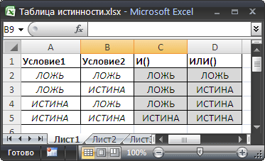
, она возвращает ЛОЖЬ, только если все ее условия ложны. Чтобы сравнить эти функции составим, так называемую таблицу истинности для
И()
и
ИЛИ()
.
Эквивалентность функции
И()
операции умножения *
В математических вычислениях EXCEL интерпретирует значение ЛОЖЬ как 0, а ИСТИНА как 1. В этом легко убедиться записав формулы
=ИСТИНА+0
и
=ЛОЖЬ+0
Следствием этого является возможность альтернативной записи формулы
=И(A1>100;A2>100)
в виде
=(A1>100)*(A2>100)
Значение второй формулы будет =1 (ИСТИНА), только если оба аргумента истинны, т.е. равны 1. Только произведение 2-х единиц даст 1 (ИСТИНА), что совпадает с определением функции
И()
.
Эквивалентность функции
И()
операции умножения * часто используется в формулах с Условием И, например, для того чтобы сложить только те значения, которые больше 5
И
меньше 10:
=СУММПРОИЗВ((A1:A10>5)*(A1:A10<10)*(A1:A10))
Проверка множества однотипных условий
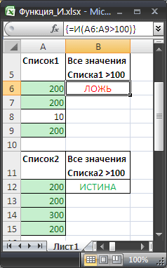
Предположим, что необходимо проверить все значения в диапазоне
A6:A9
на превышение некоторого граничного значения, например 100. Можно, конечно записать формулу
=И(A6>100;A7>100;A8>100;A9>100)
но существует более компактная формула, правда которую нужно ввести как
формулу массива
(см.
файл примера
):
=И(A6:A9>100)
(для ввода формулы в ячейку вместо
ENTER
нужно нажать
CTRL+SHIFT+ENTER
)
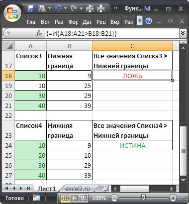
В случае, если границы для каждого проверяемого значения разные, то границы можно ввести в соседний столбец и организовать
попарное сравнение списков
с помощью
формулы массива
:
=И(A18:A21>B18:B21)
Вместо диапазона с границами можно также использовать
константу массива
:
=И(A18:A21>{9:25:29:39})