
Excel for Microsoft 365 Excel for Microsoft 365 for Mac Excel 2021 Excel 2021 for Mac Excel 2019 Excel 2019 for Mac Excel 2016 Excel 2016 for Mac Excel 2013 Excel 2010 Excel 2007 Excel for Mac 2011 More…Less
If you need to develop complex statistical or engineering analyses, you can save steps and time by using the Analysis ToolPak. You provide the data and parameters for each analysis, and the tool uses the appropriate statistical or engineering macro functions to calculate and display the results in an output table. Some tools generate charts in addition to output tables.
The data analysis functions can be used on only one worksheet at a time. When you perform data analysis on grouped worksheets, results will appear on the first worksheet and empty formatted tables will appear on the remaining worksheets. To perform data analysis on the remainder of the worksheets, recalculate the analysis tool for each worksheet.
-
Click the File tab, click Options, and then click the Add-Ins category.
If you’re using Excel 2007, click the Microsoft Office Button
 , and then click Excel Options
 -
In the Manage box, select Excel Add-ins and then click Go.
If you’re using Excel for Mac, in the file menu go to Tools > Excel Add-ins.
-
In the Add-Ins box, check the Analysis ToolPak check box, and then click OK.
-
If Analysis ToolPak is not listed in the Add-Ins available box, click Browse to locate it.
-
If you are prompted that the Analysis ToolPak is not currently installed on your computer, click Yes to install it.
-
 , and then click Excel Options
Note: To include Visual Basic for Application (VBA) functions for the Analysis ToolPak, you can load the Analysis ToolPak — VBA Add-in the same way that you load the Analysis ToolPak. In the Add-ins available box, select the Analysis ToolPak — VBA check box.
Notes:
-
The Analysis ToolPak is not available for Excel for Mac 2011. See I can’t find the Analysis ToolPak in Excel for Mac 2011 for more information.
-
Some languages aren’t supported by the Analysis ToolPak. The ToolPak displays in English when your language is not supported. See Supported languages for more information.
Load the Analysis ToolPak in Excel for Mac
-
Click the Tools menu, and then click Excel Add-ins.
-
In the Add-Ins available box, select the Analysis ToolPak check box, and then click OK.
-
If Analysis ToolPak is not listed in the Add-Ins available box, click Browse to locate it.
-
If you get a prompt that the Analysis ToolPak is not currently installed on your computer, click Yes to install it.
-
Quit and restart Excel.
Now the Data Analysis command is available on the Data tab.
-
Supported languages
|
Language |
Culture |
|
|---|---|---|
|
Chinese (Simplified) |
zh-cn |
|
|
Chinese (Traditional) |
zh-tw |
|
|
Dutch |
nl-nl |
|
|
French |
fr-fr |
|
|
French (Canadian) |
fr-CA |
|
|
Italian |
it-it |
|
|
Japanese |
ja-jp |
|
|
Norwegian (Bokmål) |
nb-no |
|
|
Polish |
pl-pl |
|
|
Portuguese |
pt-pt |
|
|
Portuguese (Brazil) |
pt-br |
|
|
Russian |
ru-ru |
|
|
Spanish |
es-es |
|
|
Spanish (Mexico) |
es-MX |
|
|
Swedish |
sv-se |
I can’t find the Analysis ToolPak in Excel for Mac 2011
There are a few third-party add-ins that provide Analysis ToolPak functionality for Excel 2011.
Option 1: Download the XLSTAT add-on statistical software for Mac and use it in Excel 2011. XLSTAT contains more than 200 basic and advanced statistical tools that include all of the Analysis ToolPak features.
-
Go to the XLSTAT download page.
-
Select the XLSTAT version that matches your Mac OS and download it.
-
Follow the MAC OS installation instructions.
-
Open the Excel file that contains your data and click on the XLSTAT icon to launch the XLSTAT toolbar.
-
For 30 days, you’ll have access to all XLSTAT functions. After 30 days you will be able to use the free version that includes the Analysis ToolPak functions, or order one of the more complete solutions of XLSTAT.
Option 2: Download StatPlus:mac LE for free from AnalystSoft, and then use StatPlus:mac LE with Excel 2011.
You can use StatPlus:mac LE to perform many of the functions that were previously available in the Analysis ToolPak, such as regressions, histograms, analysis of variance (ANOVA), and t-tests.
-
Visit the AnalystSoft Web site, and then follow the instructions on the download page.
-
After you have downloaded and installed StatPlus:mac LE, open the workbook that contains the data that you want to analyze.
-
Open StatPlus:mac LE. The functions are located on the StatPlus:mac LE menus.
Important:
-
Excel 2011 does not include Help for XLStat or StatPlus:mac LE. Help for XLStat is provided by XLSTAT. Help for StatPlus:mac LE is provided by AnalystSoft.
-
Microsoft does not provide support for either product.
-
Need more help?
You can always ask an expert in the Excel Tech Community or get support in the Answers community.
See Also
Perform statistical and engineering analysis with the Analysis ToolPak.
Need more help?
Excel for Microsoft 365 Excel for Microsoft 365 for Mac Excel 2021 Excel 2021 for Mac Excel 2019 Excel 2019 for Mac Excel 2016 Excel 2016 for Mac Excel 2013 Excel 2010 Excel 2007 More…Less
If you need to develop complex statistical or engineering analyses, you can save steps and time by using the Analysis ToolPak. You provide the data and parameters for each analysis, and the tool uses the appropriate statistical or engineering macro functions to calculate and display the results in an output table. Some tools generate charts in addition to output tables.
The data analysis functions can be used on only one worksheet at a time. When you perform data analysis on grouped worksheets, results will appear on the first worksheet and empty formatted tables will appear on the remaining worksheets. To perform data analysis on the remainder of the worksheets, recalculate the analysis tool for each worksheet.
The Analysis ToolPak includes the tools described in the following sections. To access these tools, click Data Analysis in the Analysis group on the Data tab. If the Data Analysis command is not available, you need to load the Analysis ToolPak add-in program.
-
Click the File tab, click Options, and then click the Add-Ins category.
-
In the Manage box, select Excel Add-ins and then click Go.
If you’re using Excel for Mac, in the file menu go to Tools > Excel Add-ins.
-
In the Add-Ins box, check the Analysis ToolPak check box, and then click OK.
-
If Analysis ToolPak is not listed in the Add-Ins available box, click Browse to locate it.
-
If you are prompted that the Analysis ToolPak is not currently installed on your computer, click Yes to install it.
-
Note: To include Visual Basic for Application (VBA) functions for the Analysis ToolPak, you can load the Analysis ToolPak — VBA Add-in the same way that you load the Analysis ToolPak. In the Add-ins available box, select the Analysis ToolPak — VBA check box.
The Anova analysis tools provide different types of variance analysis. The tool that you should use depends on the number of factors and the number of samples that you have from the populations that you want to test.
Anova: Single Factor
This tool performs a simple analysis of variance on data for two or more samples. The analysis provides a test of the hypothesis that each sample is drawn from the same underlying probability distribution against the alternative hypothesis that underlying probability distributions are not the same for all samples. If there are only two samples, you can use the worksheet function T.TEST. With more than two samples, there is no convenient generalization of T.TEST, and the Single Factor Anova model can be called upon instead.
Anova: Two-Factor with Replication
This analysis tool is useful when data can be classified along two different dimensions. For example, in an experiment to measure the height of plants, the plants may be given different brands of fertilizer (for example, A, B, C) and might also be kept at different temperatures (for example, low, high). For each of the six possible pairs of {fertilizer, temperature}, we have an equal number of observations of plant height. Using this Anova tool, we can test:
-
Whether the heights of plants for the different fertilizer brands are drawn from the same underlying population. Temperatures are ignored for this analysis.
-
Whether the heights of plants for the different temperature levels are drawn from the same underlying population. Fertilizer brands are ignored for this analysis.
Whether having accounted for the effects of differences between fertilizer brands found in the first bulleted point and differences in temperatures found in the second bulleted point, the six samples representing all pairs of {fertilizer, temperature} values are drawn from the same population. The alternative hypothesis is that there are effects due to specific {fertilizer, temperature} pairs over and above the differences that are based on fertilizer alone or on temperature alone.
Anova: Two-Factor Without Replication
This analysis tool is useful when data is classified on two different dimensions as in the Two-Factor case With Replication. However, for this tool it is assumed that there is only a single observation for each pair (for example, each {fertilizer, temperature} pair in the preceding example).
The CORREL and PEARSON worksheet functions both calculate the correlation coefficient between two measurement variables when measurements on each variable are observed for each of N subjects. (Any missing observation for any subject causes that subject to be ignored in the analysis.) The Correlation analysis tool is particularly useful when there are more than two measurement variables for each of N subjects. It provides an output table, a correlation matrix, that shows the value of CORREL (or PEARSON) applied to each possible pair of measurement variables.
The correlation coefficient, like the covariance, is a measure of the extent to which two measurement variables «vary together.» Unlike the covariance, the correlation coefficient is scaled so that its value is independent of the units in which the two measurement variables are expressed. (For example, if the two measurement variables are weight and height, the value of the correlation coefficient is unchanged if weight is converted from pounds to kilograms.) The value of any correlation coefficient must be between -1 and +1 inclusive.
You can use the correlation analysis tool to examine each pair of measurement variables to determine whether the two measurement variables tend to move together — that is, whether large values of one variable tend to be associated with large values of the other (positive correlation), whether small values of one variable tend to be associated with large values of the other (negative correlation), or whether values of both variables tend to be unrelated (correlation near 0 (zero)).
The Correlation and Covariance tools can both be used in the same setting, when you have N different measurement variables observed on a set of individuals. The Correlation and Covariance tools each give an output table, a matrix, that shows the correlation coefficient or covariance, respectively, between each pair of measurement variables. The difference is that correlation coefficients are scaled to lie between -1 and +1 inclusive. Corresponding covariances are not scaled. Both the correlation coefficient and the covariance are measures of the extent to which two variables «vary together.»
The Covariance tool computes the value of the worksheet function COVARIANCE.P for each pair of measurement variables. (Direct use of COVARIANCE.P rather than the Covariance tool is a reasonable alternative when there are only two measurement variables, that is, N=2.) The entry on the diagonal of the Covariance tool’s output table in row i, column i is the covariance of the i-th measurement variable with itself. This is just the population variance for that variable, as calculated by the worksheet function VAR.P.
You can use the Covariance tool to examine each pair of measurement variables to determine whether the two measurement variables tend to move together — that is, whether large values of one variable tend to be associated with large values of the other (positive covariance), whether small values of one variable tend to be associated with large values of the other (negative covariance), or whether values of both variables tend to be unrelated (covariance near 0 (zero)).
The Descriptive Statistics analysis tool generates a report of univariate statistics for data in the input range, providing information about the central tendency and variability of your data.
The Exponential Smoothing analysis tool predicts a value that is based on the forecast for the prior period, adjusted for the error in that prior forecast. The tool uses the smoothing constant a, the magnitude of which determines how strongly the forecasts respond to errors in the prior forecast.
Note: Values of 0.2 to 0.3 are reasonable smoothing constants. These values indicate that the current forecast should be adjusted 20 percent to 30 percent for error in the prior forecast. Larger constants yield a faster response but can produce erratic projections. Smaller constants can result in long lags for forecast values.
The F-Test Two-Sample for Variances analysis tool performs a two-sample F-test to compare two population variances.
For example, you can use the F-Test tool on samples of times in a swim meet for each of two teams. The tool provides the result of a test of the null hypothesis that these two samples come from distributions with equal variances, against the alternative that the variances are not equal in the underlying distributions.
The tool calculates the value f of an F-statistic (or F-ratio). A value of f close to 1 provides evidence that the underlying population variances are equal. In the output table, if f < 1 «P(F <= f) one-tail» gives the probability of observing a value of the F-statistic less than f when population variances are equal, and «F Critical one-tail» gives the critical value less than 1 for the chosen significance level, Alpha. If f > 1, «P(F <= f) one-tail» gives the probability of observing a value of the F-statistic greater than f when population variances are equal, and «F Critical one-tail» gives the critical value greater than 1 for Alpha.
The Fourier Analysis tool solves problems in linear systems and analyzes periodic data by using the Fast Fourier Transform (FFT) method to transform data. This tool also supports inverse transformations, in which the inverse of transformed data returns the original data.
The Histogram analysis tool calculates individual and cumulative frequencies for a cell range of data and data bins. This tool generates data for the number of occurrences of a value in a data set.
For example, in a class of 20 students, you can determine the distribution of scores in letter-grade categories. A histogram table presents the letter-grade boundaries and the number of scores between the lowest bound and the current bound. The single most-frequent score is the mode of the data.
Tip: In Excel 2016, you can now create a histogram or Pareto chart.
The Moving Average analysis tool projects values in the forecast period, based on the average value of the variable over a specific number of preceding periods. A moving average provides trend information that a simple average of all historical data would mask. Use this tool to forecast sales, inventory, or other trends. Each forecast value is based on the following formula.
where:
-
N is the number of prior periods to include in the moving average
-
A
j is the actual value at time j -
F
j is the forecasted value at time j
The Random Number Generation analysis tool fills a range with independent random numbers that are drawn from one of several distributions. You can characterize the subjects in a population with a probability distribution. For example, you can use a normal distribution to characterize the population of individuals’ heights, or you can use a Bernoulli distribution of two possible outcomes to characterize the population of coin-flip results.
The Rank and Percentile analysis tool produces a table that contains the ordinal and percentage rank of each value in a data set. You can analyze the relative standing of values in a data set. This tool uses the worksheet functions RANK.EQ andPERCENTRANK.INC. If you want to account for tied values, use the RANK.EQ function, which treats tied values as having the same rank, or use the RANK.AVG function, which returns the average rank for the tied values.
The Regression analysis tool performs linear regression analysis by using the «least squares» method to fit a line through a set of observations. You can analyze how a single dependent variable is affected by the values of one or more independent variables. For example, you can analyze how an athlete’s performance is affected by such factors as age, height, and weight. You can apportion shares in the performance measure to each of these three factors, based on a set of performance data, and then use the results to predict the performance of a new, untested athlete.
The Regression tool uses the worksheet function LINEST.
The Sampling analysis tool creates a sample from a population by treating the input range as a population. When the population is too large to process or chart, you can use a representative sample. You can also create a sample that contains only the values from a particular part of a cycle if you believe that the input data is periodic. For example, if the input range contains quarterly sales figures, sampling with a periodic rate of four places the values from the same quarter in the output range.
The Two-Sample t-Test analysis tools test for equality of the population means that underlie each sample. The three tools employ different assumptions: that the population variances are equal, that the population variances are not equal, and that the two samples represent before-treatment and after-treatment observations on the same subjects.
For all three tools below, a t-Statistic value, t, is computed and shown as «t Stat» in the output tables. Depending on the data, this value, t, can be negative or nonnegative. Under the assumption of equal underlying population means, if t < 0, «P(T <= t) one-tail» gives the probability that a value of the t-Statistic would be observed that is more negative than t. If t >=0, «P(T <= t) one-tail» gives the probability that a value of the t-Statistic would be observed that is more positive than t. «t Critical one-tail» gives the cutoff value, so that the probability of observing a value of the t-Statistic greater than or equal to «t Critical one-tail» is Alpha.
«P(T <= t) two-tail» gives the probability that a value of the t-Statistic would be observed that is larger in absolute value than t. «P Critical two-tail» gives the cutoff value, so that the probability of an observed t-Statistic larger in absolute value than «P Critical two-tail» is Alpha.
t-Test: Paired Two Sample For Means
You can use a paired test when there is a natural pairing of observations in the samples, such as when a sample group is tested twice — before and after an experiment. This analysis tool and its formula perform a paired two-sample Student’s t-Test to determine whether observations that are taken before a treatment and observations taken after a treatment are likely to have come from distributions with equal population means. This t-Test form does not assume that the variances of both populations are equal.
Note: Among the results that are generated by this tool is pooled variance, an accumulated measure of the spread of data about the mean, which is derived from the following formula.
t-Test: Two-Sample Assuming Equal Variances
This analysis tool performs a two-sample student’s t-Test. This t-Test form assumes that the two data sets came from distributions with the same variances. It is referred to as a homoscedastic t-Test. You can use this t-Test to determine whether the two samples are likely to have come from distributions with equal population means.
t-Test: Two-Sample Assuming Unequal Variances
This analysis tool performs a two-sample student’s t-Test. This t-Test form assumes that the two data sets came from distributions with unequal variances. It is referred to as a heteroscedastic t-Test. As with the preceding Equal Variances case, you can use this t-Test to determine whether the two samples are likely to have come from distributions with equal population means. Use this test when there are distinct subjects in the two samples. Use the Paired test, described in the follow example, when there is a single set of subjects and the two samples represent measurements for each subject before and after a treatment.
The following formula is used to determine the statistic value t.
The following formula is used to calculate the degrees of freedom, df. Because the result of the calculation is usually not an integer, the value of df is rounded to the nearest integer to obtain a critical value from the t table. The Excel worksheet function T.TEST uses the calculated df value without rounding, because it is possible to compute a value for T.TEST with a noninteger df. Because of these different approaches to determining the degrees of freedom, the results of T.TEST and this t-Test tool will differ in the Unequal Variances case.
The z-Test: Two Sample for Means analysis tool performs a two sample z-Test for means with known variances. This tool is used to test the null hypothesis that there is no difference between two population means against either one-sided or two-sided alternative hypotheses. If variances are not known, the worksheet function Z.TEST should be used instead.
When you use the z-Test tool, be careful to understand the output. «P(Z <= z) one-tail» is really P(Z >= ABS(z)), the probability of a z-value further from 0 in the same direction as the observed z value when there is no difference between the population means. «P(Z <= z) two-tail» is really P(Z >= ABS(z) or Z <= -ABS(z)), the probability of a z-value further from 0 in either direction than the observed z-value when there is no difference between the population means. The two-tailed result is just the one-tailed result multiplied by 2. The z-Test tool can also be used for the case where the null hypothesis is that there is a specific nonzero value for the difference between the two population means. For example, you can use this test to determine differences between the performances of two car models.
Need more help?
You can always ask an expert in the Excel Tech Community or get support in the Answers community.
See Also
Create a histogram in Excel 2016
Create a Pareto chart in Excel 2016
Load the Analysis ToolPak in Excel
ENGINEERING functions (reference)
Overview of formulas in Excel
How to avoid broken formulas
Find and correct errors in formulas
Excel keyboard shortcuts and function keys
Excel functions (alphabetical)
Excel functions (by category)
Need more help?
17 авг. 2022 г.
читать 1 мин
Analysis ToolPak — это бесплатная надстройка Microsoft Excel, которая предоставляет инструменты, необходимые для выполнения сложных статистических, финансовых или инженерных анализов.
Чтобы загрузить пакет инструментов анализа, просто выполните следующие действия:
1. Щелкните вкладку « Файл » в левом верхнем углу, затем щелкните « Параметры » .
- В разделе « Надстройки » нажмите « Пакет анализа», затем нажмите «Перейти» .
3. Установите флажок « Пакет анализа » и нажмите « ОК ».
- На вкладке « Данные » в группе « Анализ » теперь у вас есть возможность щелкнуть « Анализ данных» , что даст вам возможность выполнять множество сложных анализов.
Написано
![]()
Замечательно! Вы успешно подписались.
Добро пожаловать обратно! Вы успешно вошли
Вы успешно подписались на кодкамп.
Срок действия вашей ссылки истек.
Ура! Проверьте свою электронную почту на наличие волшебной ссылки для входа.
Успех! Ваша платежная информация обновлена.
Ваша платежная информация не была обновлена.
Just like the other add-ins and analysis tools, the Analysis Toolpak can only be used on one worksheet at a time, which means that any evaluations are based on the active worksheet and cross-referencing will not work. The Toolpak is an add-in that you must first install before you can use it. With this tool, you can create charts about your current statistical data.
You would use this tool if you want more statistical analysis on your data. Excel 2019 isn’t made for hardcore statistics. It’s more of a simple data storage and analysis application based on formulas you create. Complex formulas can be difficult to create in Excel, and there is no reason to recreate what has already been done using the Analysis Toolpak. The Toolpak is mainly used by statisticians that want to perform calculations for t-tests, chi-square tests and correlations. With Excel, a non-statistician can perform these actions without knowing the formulas to create them. Even a statistician can take advantage of these tools by saving time writing formulas for complex analysis.
The Analysis Toolpak has several tools. Some are more commonly used than others, and some of them are better understood by laymen that just need simple analysis. The common ones that are closer to basic analysis will be explained in this article.
Installing the Analysis Toolpak
Installing the Analysis Toolpak is similar to installing the Solver tool. With your spreadsheet file open, click the «File» tab, which brings you to a window where you can set configurations on your global Excel interface. Click the «Options» button located in the left-bottom corner.
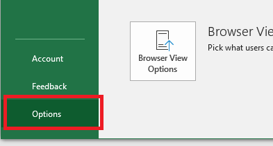
(Options button)
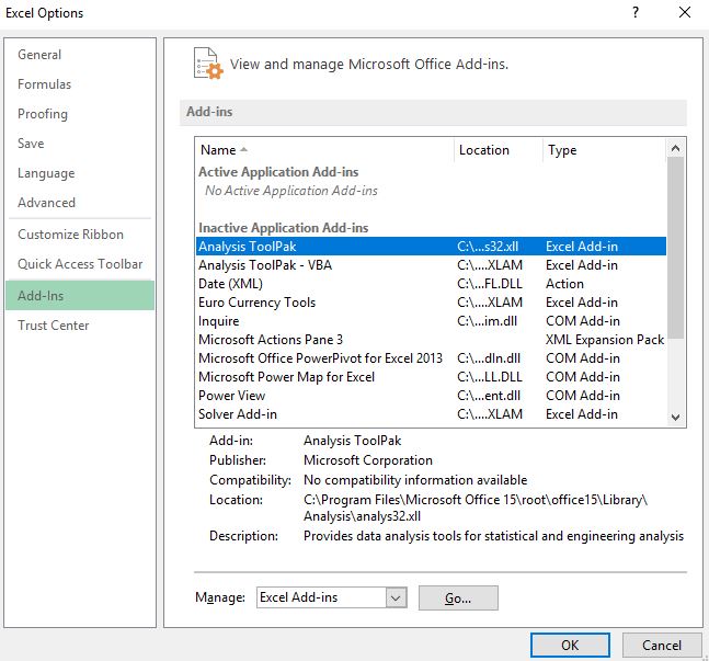
A window opens where you can configure Excel preferences including add-ins. Click the «Add-Ins» in the left panel.
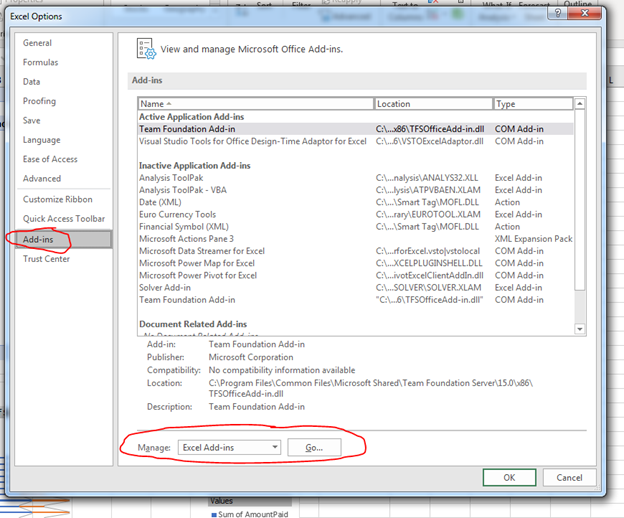
(Excel 2019 configuration window)
The «Add-ins» window shows the currently installed add-ins, but it’s also the place where you can install new plugins. In the «Manage» section, make sure the «Excel Add-ins» option is selected, and then click the «Go» button. A window opens where you choose the add-in that you want to install.
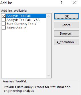
(Add-ins install choices)
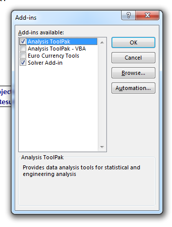
If you already installed the Solver add-in, you’ll see that it’s checked. To install the Analysis Toolpack tool, check the box next to its name and click «OK.» If it’s already installed, the tool will have a checkmark next to it. If it’s already installed, you can click «Cancel» to close the window as well.
It takes only a few seconds for the Analysis Toolpak tool to install, and when Excel is finished installing it, you’re returned to the main Excel interface. Return to the worksheet that contains your data, and you’re now ready to use the tool for analysis.
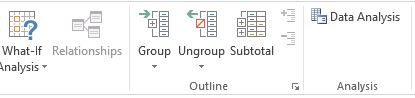
After installing the tool, the button to use it is found in the same location as the Solver tool. Click the «Data» tab in the main Excel interface, and the «Data Analysis» button can be found in the «Analyze» section of the menu.
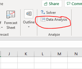
(Data Analysis button)
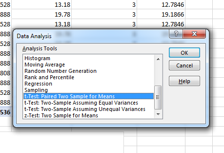
Clicking the «Data Analysis» button opens a window where all analysis tools are shown. You choose one of these tools, and then a new window will open that asks you to enter configurations specific to the chosen tool.
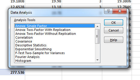
(Choose a tool)
When you look in the list of tools, you might wonder which one to choose. The one you choose depends on your goals and the information that you want to analyze. After a description of common tools, then you can make a decision on the tool that is best for your spreadsheet and goals.
Descriptive Statistics: The Descriptive Statistics tool is probably the simplest and easily understood option for viewers who need to get a mean, median, variance and standard deviation. It also offers a variety of other statistic options, but these values are the most common users are interested in when they are looking for information from worksheet data.
The mean is the average value. It’s a statistician’s way of explaining the average. The median is the middle value in a set of numbers. Standard deviation explains how spread apart numbers are from the mean. It’s a way to get an average with values that are close to this average to give you an idea of what is standard vs values that stand as outliers. Variance is related to standard deviation as standard deviation is the square root of variance. Variance is the squared value of the average of all values.
You can get a better idea of these values looking at an example. The example spreadsheet has a list of values that represent membership fees for the month of February. You can get an average from these numbers, a median and get an idea of what days are outliers using the Descriptive Statistics tool.
Click the «Descriptive Statistics» option in the Analysis Toolpak list of tools and click «OK.» A window opens where you configure the tool.
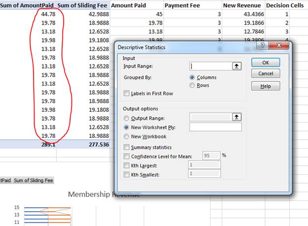
(Descriptive Statistics configuration)
The Descriptive Statistics tool requires an input range and the location of where you want to display output. The cell range that contains the total amount of revenue made for each day will be analyzed. This cell range should be entered in the «Input Range» text box. These values are organized as a column, so the default «Grouped By» value of «Columns» can be left as is. If you have values in a row of cells, this value would be switched to «Rows.»
This column of values has a header cell, so check the box labeled «Labels in First Row» so that the Analysis Toolpak tool knows to treat it as a header and not part of the data. The «Output Range» option lets you choose a range of cells where the tool will give you output after its analysis. You’ll need at least 2 columns to print out a summary, so make sure the output range has enough room for Excel to print out results.
Finally, check the box labeled «Summary» statistics to get a brief summary of your analyzed data. Then click the «Confidence Level for Mean» and leave the default value at «95,» which is already filled out for you. After you are done configuring the tool, click «OK» and Excel takes a few seconds to analyze data and display it in the output cell range that you specified in the configuration window.
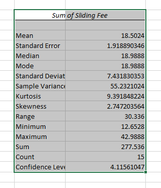
(Descriptive Statistics report)
The report gives you values for several statistical data points. The mean is the average and usually the most important value in this report that most reviewers are looking for. The average in this report is about 18.5, which means that the average revenue for the data range is $18.50 for the month.
Median and Mode in this report are the same number. The median is the middle value in the list of values. The Mode is the value that appears the most in the list of values. The standard deviation helps you identify outliers. You add the standard deviation to the mean, and then subtract the standard deviation value to the mean. This gives you a range of values that you can identify as standard revenue for the month of February.
The minimum and maximum are the highs and lows in your data range. The sum value is just the added values to give you a total, and the count is the number of values within the range. Use this Analysis Toolpak tool to get basic statistic information from your data, and it’s one of the easiest tools to you. It’s the most used of all the tools because it’s simple data that can be easily understand by business owners.
The t-Test Tool
A t-test is beneficial when you want to compare two sample data points. In Excel 2019, it’s useful when you want to compare two columns or two rows. For instance, you might want to compare values before and after an event or before and after a marketing campaign.
In the example spreadsheet, there are two columns with different revenue. The sliding fee column displays revenue based on the amount of revenue affecting the payment fee. The «New Revenue» is an altered version of revenue based on goal tools. You can do a comparison between the two columns using a t-test. You could write your own formula and set up each cell individually and manually, or you can use Excel’s Analysis Toolpak tool.
Click the «Data Analysis» button to open a window with a list of tool choices.
(Analysis Toolkit options)
Choose the tool named «t-Test: Paired Two Sample for Means» and then click the «OK» button. This selection opens a new configuration window where you set up the tool to work with your data.
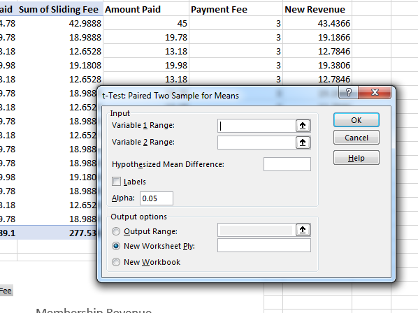
(T-Test configuration)
The «Input» section contains input text boxes where you choose the two columns to compare. In this example, the sliding fee column will be compared to the new revenue column to determine the basic difference between the two. Enter the cell range for the first column in the «Variable 1 Range» text box. Then, enter the second cell range in the input text box labeled «Variable 2 Range.»
Change the «Output options» section to the «Output range» option so that you can see the report results in the same worksheet. After you are finished configuring the t-test tool, click the «OK» button to run the analysis. It only takes a few seconds for Excel to generate the report and display it in the selected output cells.
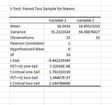
(T-Test results)
The most important output to get out of this report is the mean value. This value lets you see the average difference between the two columns. Using the comparison, you can determine which section has the best average between the two and lets you determine which column of values have the best output for your decision-making results.
Take note of the «P(T<=t) one-tail» value. This is your P value. If this value is less than .05, then your values are significantly different and possibly unrelated, so you should choose different cell range values to work with your analysis.
The ANOVA Tool
The ANOVA tools in Excel 2019 analyze variance. Variance is important in statistics because it determines outliers in data and gives you a bigger picture of relevant data. The ANOVA tool lets you identify if there is a relationship between two sets of data. For this example, the ANOVA single factor tool will be used, but you can use ANOVA tools for two-factor analysis similar to a t-test. The two-factor version of the ANOVA tool checks two independent variables, and you can indicate that you want to use a tool with or without replication. For simple analysis of two dependent variables, you use single factor. Take note that single factor is for dependent variables and any two-factor tools are used on independent variables.
Click the «Data Analysis» button again. The same window opens where you choose a tool. Choose «ANOVA: Single Factor» and a new configuration window displays. This window is where you configure the tool’s input to determine the report results.
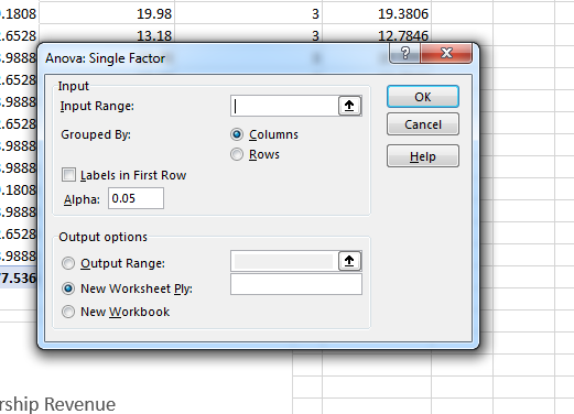
(ANOVA configuration)
In the configuration window, you choose an input range. This range should be two adjacent columns. The sample spreadsheet has columns of revenue based on membership fees. Because they are dependent, this analysis tool is best for this worksheet data. Choose one of the column cell ranges, and then leave the «Columns» option in the «Grouped By» section.
Change the «Output options» section to the «Output Range» open and choose the cells where you want to display your output. After you are finished configuring your tool settings, click the «OK» button to run the report. Excel runs the report quickly when you only have a few values to analyze. The result is displayed in the selected output cells.
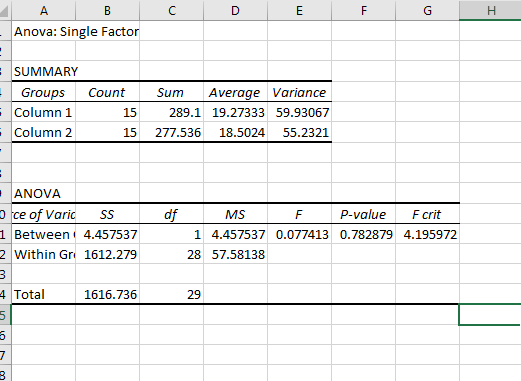
(ANOVA report)
The summary section displays a comparison chart of the two columns, but the value to take note of is the P value. Again, if this value is below .05, then you have unrelated data and these values should be adjusted. You would then need to choose a different set of records, select them and re-run the ANOVA report.
The Analysis Toolpak has numerous other reports, but these tools are the most common and most useful for users who are looking for some quick analysis on data. You can test other tools by selecting them in the data analysis tool selection window, configuring values located in your spreadsheet and running a new report.
Analysis Toolpak is a kind of add-in Microsoft Excel that allows users to use data analysis tools for statistical and engineering analysis. The Analysis Toolpak consists of 19 functional tools that can be used to do statistical/engineering analysis. Given below is a table that includes names of all the functional tools available under Analysis Toolpak:
| 1. Anova: Single Factor | 2. Anova: Two-Factor with Replication | 3. Anova: Two-Factor Without Replication |
| 4. Correlation | 5. Covariance | 6. Descriptive Statistics |
| 7. Exponential Smoothing | 8. F-Test Two-Sample for Variance | 9. Fourier Analysis |
| 10. Histogram | 11. Moving Average | 12. Random Number Generation |
| 13. Rank and Percents | 14. Regression | 15. Sampling |
| 16. t-Test: Paired Two Sample for Means | 17. t-Test: Two-Sample Assuming Equal Variances | 18. t-Test: Two-Sample Assuming Unequal Variances |
| 19. Z-Test: Two-Samples for Mean |
But to use these tools, we need to install the Analysis Toolpak in our Microsoft Excel. In this article, we are going to learn how can we install it depending on whether you are using Excel or Mac.
Installing Analysis Toolpak in Excel in macOS
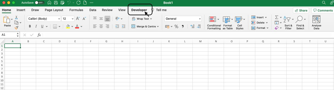
Step 1: In the ribbons present on the top of the Excel window, click on the Developer tab.
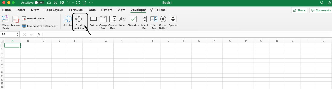
Step 2: In the Developer tab, locate the option “Excel Add-ins” and click on it to open the Add-ins dialog box.
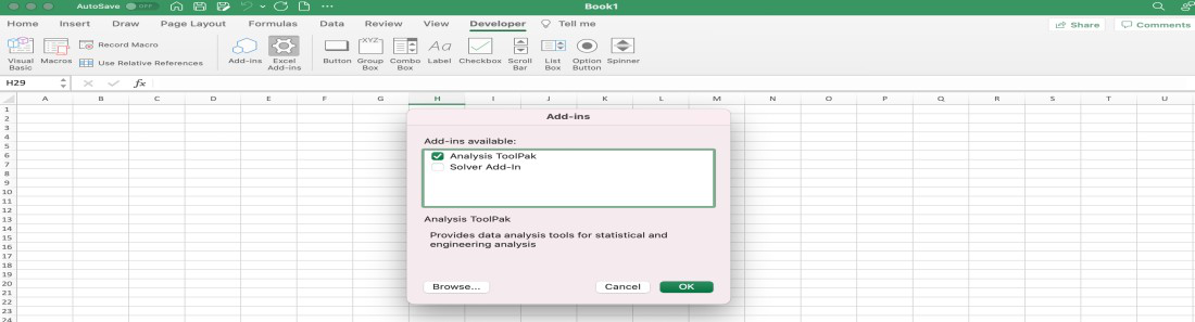
Step 3: In the Add-ins dialog box, we can see the available add-in options. If the Analysis ToolPak option checkbox is not ticked, click on the checkbox to make it green and then click the OK button.
Step 4: Now, go to the top ribbon and select the Data tab. In the Data tab, the Data Analysis option will become visible.

Step 5: On clicking the Data Analysis option, we can see the Analysis Tools dialog box which contains all the functional tool options.
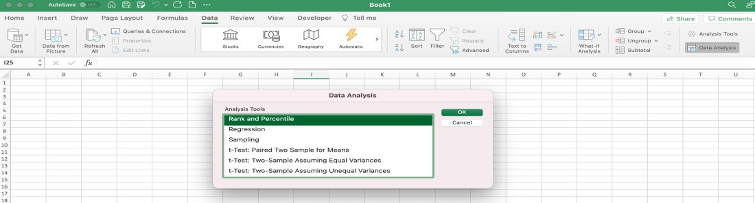
A video displaying each of the above steps is also attached below.
Installing Analysis Toolpak in Excel on Windows
Step 1: In the ribbons present on the top of the Excel window, click on the File button.

Step 2: A new window will appear, from the left-hand side of the window, look out for the “Options” button and click on it to open it.

Step 3: A dialog box named “Excel options” will appear on the screen. From the left-hand side of the box, locate the “Add-ins” option and click on it.

Step 4: Under the “Manage” option, select “Excel Add-ins” from the drop-down menu and click on the Go button to open the Add-ins dialog box.

Step 5: In the Add-ins dialog box, we can see the available add-in options. If the Analysis ToolPak option checkbox is not ticked, click on the checkbox to make it green and then click the OK button.

Step 6: Now, go to the top ribbon and select the Data tab. In the Data tab, the Data Analysis option will become visible.

Step 7: On clicking the Data Analysis option, we can see the Analysis Tools dialog box which contains all the functional tool options.

Note: Sometimes, an installation prompt is shown to the user that says the Analysis ToolPak is not currently installed on your system, click Yes to install it. In such cases, the user should accept the request to install the Analysis Toolpak.