
ABS function
Math and trigonometry: Returns the absolute value of a number
ACCRINT function
Financial: Returns the accrued interest for a security that pays periodic interest
ACCRINTM function
Financial: Returns the accrued interest for a security that pays interest at maturity
ACOS function
Math and trigonometry: Returns the arccosine of a number
ACOSH function
Math and trigonometry: Returns the inverse hyperbolic cosine of a number
ACOT function

Math and trigonometry: Returns the arccotangent of a number
ACOTH function
Math and trigonometry: Returns the hyperbolic arccotangent of a number
AGGREGATE function
Math and trigonometry: Returns an aggregate in a list or database
ADDRESS function
Lookup and reference: Returns a reference as text to a single cell in a worksheet
AMORDEGRC function
Financial: Returns the depreciation for each accounting period by using a depreciation coefficient
AMORLINC function
Financial: Returns the depreciation for each accounting period
AND function
Logical: Returns TRUE if all of its arguments are TRUE
ARABIC function
Math and trigonometry: Converts a Roman number to Arabic, as a number
AREAS function
Lookup and reference: Returns the number of areas in a reference
ARRAYTOTEXT function

Text: Returns an array of text values from any specified range
ASC function
Text: Changes full-width (double-byte) English letters or katakana within a character string to half-width (single-byte) characters
ASIN function
Math and trigonometry: Returns the arcsine of a number
ASINH function
Math and trigonometry: Returns the inverse hyperbolic sine of a number
ATAN function
Math and trigonometry: Returns the arctangent of a number
ATAN2 function
Math and trigonometry: Returns the arctangent from x- and y-coordinates
ATANH function
Math and trigonometry: Returns the inverse hyperbolic tangent of a number
AVEDEV function
Statistical: Returns the average of the absolute deviations of data points from their mean
AVERAGE function
Statistical: Returns the average of its arguments
AVERAGEA function
Statistical: Returns the average of its arguments, including numbers, text, and logical values
AVERAGEIF function
Statistical: Returns the average (arithmetic mean) of all the cells in a range that meet a given criteria
AVERAGEIFS function
Statistical: Returns the average (arithmetic mean) of all cells that meet multiple criteria.
BAHTTEXT function
Text: Converts a number to text, using the ß (baht) currency format
BASE function
Math and trigonometry: Converts a number into a text representation with the given radix (base)
BESSELI function
Engineering: Returns the modified Bessel function In(x)
BESSELJ function
Engineering: Returns the Bessel function Jn(x)
BESSELK function
Engineering: Returns the modified Bessel function Kn(x)
BESSELY function
Engineering: Returns the Bessel function Yn(x)
BETADIST function
Compatibility: Returns the beta cumulative distribution function
In Excel 2007, this is a Statistical function.
BETA.DIST function

Statistical: Returns the beta cumulative distribution function
BETAINV function
Compatibility: Returns the inverse of the cumulative distribution function for a specified beta distribution
In Excel 2007, this is a Statistical function.
BETA.INV function
Statistical: Returns the inverse of the cumulative distribution function for a specified beta distribution
BIN2DEC function
Engineering: Converts a binary number to decimal
BIN2HEX function
Engineering: Converts a binary number to hexadecimal
BIN2OCT function
Engineering: Converts a binary number to octal
BINOMDIST function
Compatibility: Returns the individual term binomial distribution probability
In Excel 2007, this is a Statistical function.
BINOM.DIST function
Statistical: Returns the individual term binomial distribution probability
BINOM.DIST.RANGE function
Statistical: Returns the probability of a trial result using a binomial distribution
BINOM.INV function
Statistical: Returns the smallest value for which the cumulative binomial distribution is less than or equal to a criterion value
BITAND function
Engineering: Returns a ‘Bitwise And’ of two numbers
BITLSHIFT function
Engineering: Returns a value number shifted left by shift_amount bits
BITOR function
Engineering: Returns a bitwise OR of 2 numbers
BITRSHIFT function
Engineering: Returns a value number shifted right by shift_amount bits
BITXOR function
Engineering: Returns a bitwise ‘Exclusive Or’ of two numbers
BYCOL
Logical: Applies a LAMBDA to each column and returns an array of the results
BYROW
Logical: Applies a LAMBDA to each row and returns an array of the results
CALL function
Add-in and Automation: Calls a procedure in a dynamic link library or code resource
CEILING function
Compatibility: Rounds a number to the nearest integer or to the nearest multiple of significance
CEILING.MATH function
Math and trigonometry: Rounds a number up, to the nearest integer or to the nearest multiple of significance
CEILING.PRECISE function
Math and trigonometry: Rounds a number the nearest integer or to the nearest multiple of significance. Regardless of the sign of the number, the number is rounded up.
CELL function
Information: Returns information about the formatting, location, or contents of a cell
This function is not available in Excel for the web.
CHAR function
Text: Returns the character specified by the code number
CHIDIST function
Compatibility: Returns the one-tailed probability of the chi-squared distribution
Note: In Excel 2007, this is a Statistical function.
CHIINV function
Compatibility: Returns the inverse of the one-tailed probability of the chi-squared distribution
Note: In Excel 2007, this is a Statistical function.
CHITEST function
Compatibility: Returns the test for independence
Note: In Excel 2007, this is a Statistical function.
CHISQ.DIST function
Statistical: Returns the cumulative beta probability density function
CHISQ.DIST.RT function
Statistical: Returns the one-tailed probability of the chi-squared distribution
CHISQ.INV function
Statistical: Returns the cumulative beta probability density function
CHISQ.INV.RT function
Statistical: Returns the inverse of the one-tailed probability of the chi-squared distribution
CHISQ.TEST function
Statistical: Returns the test for independence
CHOOSE function
Lookup and reference: Chooses a value from a list of values
CHOOSECOLS
Lookup and reference: Returns the specified columns from an array
CHOOSEROWS
Lookup and reference: Returns the specified rows from an array
CLEAN function
Text: Removes all nonprintable characters from text
CODE function
Text: Returns a numeric code for the first character in a text string
COLUMN function
Lookup and reference: Returns the column number of a reference
COLUMNS function
Lookup and reference: Returns the number of columns in a reference
COMBIN function
Math and trigonometry: Returns the number of combinations for a given number of objects
COMBINA function
Math and trigonometry:
Returns the number of combinations with repetitions for a given number of items
COMPLEX function
Engineering: Converts real and imaginary coefficients into a complex number
CONCAT function

Text: Combines the text from multiple ranges and/or strings, but it doesn’t provide the delimiter or IgnoreEmpty arguments.
CONCATENATE function
Text: Joins several text items into one text item
CONFIDENCE function
Compatibility: Returns the confidence interval for a population mean
In Excel 2007, this is a Statistical function.
CONFIDENCE.NORM function
Statistical: Returns the confidence interval for a population mean
CONFIDENCE.T function
Statistical: Returns the confidence interval for a population mean, using a Student’s t distribution
CONVERT function
Engineering: Converts a number from one measurement system to another
CORREL function
Statistical: Returns the correlation coefficient between two data sets
COS function
Math and trigonometry: Returns the cosine of a number
COSH function
Math and trigonometry: Returns the hyperbolic cosine of a number
COT function
Math and trigonometry: Returns the hyperbolic cosine of a number
COTH function
Math and trigonometry: Returns the cotangent of an angle
COUNT function
Statistical: Counts how many numbers are in the list of arguments
COUNTA function
Statistical: Counts how many values are in the list of arguments
COUNTBLANK function
Statistical: Counts the number of blank cells within a range
COUNTIF function
Statistical: Counts the number of cells within a range that meet the given criteria
COUNTIFS function
Statistical: Counts the number of cells within a range that meet multiple criteria
COUPDAYBS function
Financial: Returns the number of days from the beginning of the coupon period to the settlement date
COUPDAYS function
Financial: Returns the number of days in the coupon period that contains the settlement date
COUPDAYSNC function
Financial: Returns the number of days from the settlement date to the next coupon date
COUPNCD function
Financial: Returns the next coupon date after the settlement date
COUPNUM function
Financial: Returns the number of coupons payable between the settlement date and maturity date
COUPPCD function
Financial: Returns the previous coupon date before the settlement date
COVAR function
Compatibility: Returns covariance, the average of the products of paired deviations
In Excel 2007, this is a Statistical function.
COVARIANCE.P function
Statistical: Returns covariance, the average of the products of paired deviations
COVARIANCE.S function
Statistical: Returns the sample covariance, the average of the products deviations for each data point pair in two data sets
CRITBINOM function
Compatibility: Returns the smallest value for which the cumulative binomial distribution is less than or equal to a criterion value
In Excel 2007, this is a Statistical function.
CSC function
Math and trigonometry: Returns the cosecant of an angle
CSCH function
Math and trigonometry: Returns the hyperbolic cosecant of an angle
CUBEKPIMEMBER function
Cube: Returns a key performance indicator (KPI) name, property, and measure, and displays the name and property in the cell. A KPI is a quantifiable measurement, such as monthly gross profit or quarterly employee turnover, used to monitor an organization’s performance.
CUBEMEMBER function
Cube: Returns a member or tuple in a cube hierarchy. Use to validate that the member or tuple exists in the cube.
CUBEMEMBERPROPERTY function
Cube: Returns the value of a member property in the cube. Use to validate that a member name exists within the cube and to return the specified property for this member.
CUBERANKEDMEMBER function
Cube: Returns the nth, or ranked, member in a set. Use to return one or more elements in a set, such as the top sales performer or top 10 students.
CUBESET function
Cube: Defines a calculated set of members or tuples by sending a set expression to the cube on the server, which creates the set, and then returns that set to Microsoft Office Excel.
CUBESETCOUNT function
Cube: Returns the number of items in a set.
CUBEVALUE function
Cube: Returns an aggregated value from a cube.
CUMIPMT function
Financial: Returns the cumulative interest paid between two periods
CUMPRINC function
Financial: Returns the cumulative principal paid on a loan between two periods
DATE function
Date and time: Returns the serial number of a particular date
DATEDIF function
Date and time: Calculates the number of days, months, or years between two dates. This function is useful in formulas where you need to calculate an age.
DATEVALUE function
Date and time: Converts a date in the form of text to a serial number
DAVERAGE function
Database: Returns the average of selected database entries
DAY function
Date and time: Converts a serial number to a day of the month
DAYS function
Date and time: Returns the number of days between two dates
DAYS360 function
Date and time: Calculates the number of days between two dates based on a 360-day year
DB function
Financial: Returns the depreciation of an asset for a specified period by using the fixed-declining balance method
DBCS function
Text: Changes half-width (single-byte) English letters or katakana within a character string to full-width (double-byte) characters
DCOUNT function
Database: Counts the cells that contain numbers in a database
DCOUNTA function
Database: Counts nonblank cells in a database
DDB function
Financial: Returns the depreciation of an asset for a specified period by using the double-declining balance method or some other method that you specify
DEC2BIN function
Engineering: Converts a decimal number to binary
DEC2HEX function
Engineering: Converts a decimal number to hexadecimal
DEC2OCT function
Engineering: Converts a decimal number to octal
DECIMAL function
Math and trigonometry: Converts a text representation of a number in a given base into a decimal number
DEGREES function
Math and trigonometry: Converts radians to degrees
DELTA function
Engineering: Tests whether two values are equal
DEVSQ function
Statistical: Returns the sum of squares of deviations
DGET function
Database: Extracts from a database a single record that matches the specified criteria
DISC function
Financial: Returns the discount rate for a security
DMAX function
Database: Returns the maximum value from selected database entries
DMIN function
Database: Returns the minimum value from selected database entries
DOLLAR function
Text: Converts a number to text, using the $ (dollar) currency format
DOLLARDE function
Financial: Converts a dollar price, expressed as a fraction, into a dollar price, expressed as a decimal number
DOLLARFR function
Financial: Converts a dollar price, expressed as a decimal number, into a dollar price, expressed as a fraction
DPRODUCT function
Database: Multiplies the values in a particular field of records that match the criteria in a database
DROP
Lookup and reference: Excludes a specified number of rows or columns from the start or end of an array
DSTDEV function
Database: Estimates the standard deviation based on a sample of selected database entries
DSTDEVP function
Database: Calculates the standard deviation based on the entire population of selected database entries
DSUM function
Database: Adds the numbers in the field column of records in the database that match the criteria
DURATION function
Financial: Returns the annual duration of a security with periodic interest payments
DVAR function
Database: Estimates variance based on a sample from selected database entries
DVARP function
Database: Calculates variance based on the entire population of selected database entries
EDATE function
Date and time: Returns the serial number of the date that is the indicated number of months before or after the start date
EFFECT function
Financial: Returns the effective annual interest rate
ENCODEURL function
Web: Returns a URL-encoded string
This function is not available in Excel for the web.
EOMONTH function
Date and time: Returns the serial number of the last day of the month before or after a specified number of months
ERF function
Engineering: Returns the error function
ERF.PRECISE function
Engineering: Returns the error function
ERFC function
Engineering: Returns the complementary error function
ERFC.PRECISE function
Engineering: Returns the complementary ERF function integrated between x and infinity
ERROR.TYPE function
Information: Returns a number corresponding to an error type
EUROCONVERT function
Add-in and Automation: Converts a number to euros, converts a number from euros to a euro member currency, or converts a number from one euro member currency to another by using the euro as an intermediary (triangulation).
EVEN function
Math and trigonometry: Rounds a number up to the nearest even integer
EXACT function
Text: Checks to see if two text values are identical
EXP function
Math and trigonometry: Returns e raised to the power of a given number
EXPAND
Lookup and reference: Expands or pads an array to specified row and column dimensions
EXPON.DIST function
Statistical: Returns the exponential distribution
EXPONDIST function
Compatibility: Returns the exponential distribution
In Excel 2007, this is a Statistical function.
FACT function
Math and trigonometry: Returns the factorial of a number
FACTDOUBLE function
Math and trigonometry: Returns the double factorial of a number
FALSE function
Logical: Returns the logical value FALSE
F.DIST function
Statistical: Returns the F probability distribution
FDIST function
Compatibility: Returns the F probability distribution
In Excel 2007, this is a Statistical function.
F.DIST.RT function
Statistical: Returns the F probability distribution
FILTER function
Lookup and reference: Filters a range of data based on criteria you define
FILTERXML function
Web: Returns specific data from the XML content by using the specified XPath
This function is not available in Excel for the web.
FIND, FINDB functions
Text: Finds one text value within another (case-sensitive)
F.INV function
Statistical: Returns the inverse of the F probability distribution
F.INV.RT function
Statistical: Returns the inverse of the F probability distribution
FINV function
Compatibility: Returns the inverse of the F probability distribution
In Excel 2007this is a Statistical function.
FISHER function
Statistical: Returns the Fisher transformation
FISHERINV function
Statistical: Returns the inverse of the Fisher transformation
FIXED function
Text: Formats a number as text with a fixed number of decimals
FLOOR function
Compatibility: Rounds a number down, toward zero
In Excel 2007 and Excel 2010, this is a Math and trigonometry function.
FLOOR.MATH function
Math and trigonometry: Rounds a number down, to the nearest integer or to the nearest multiple of significance
FLOOR.PRECISE function
Math and trigonometry: Rounds a number the nearest integer or to the nearest multiple of significance. Regardless of the sign of the number, the number is rounded up.
FORECAST function
Statistical: Returns a value along a linear trend
In Excel 2016, this function is replaced with FORECAST.LINEAR as part of the new Forecasting functions, but it’s still available for compatibility with earlier versions.
FORECAST.ETS function

Statistical: Returns a future value based on existing (historical) values by using the AAA version of the Exponential Smoothing (ETS) algorithm
FORECAST.ETS.CONFINT function
Statistical: Returns a confidence interval for the forecast value at the specified target date
FORECAST.ETS.SEASONALITY function
Statistical: Returns the length of the repetitive pattern Excel detects for the specified time series
FORECAST.ETS.STAT function
Statistical: Returns a statistical value as a result of time series forecasting
FORECAST.LINEAR function
Statistical: Returns a future value based on existing values
FORMULATEXT function
Lookup and reference: Returns the formula at the given reference as text
FREQUENCY function
Statistical: Returns a frequency distribution as a vertical array
F.TEST function
Statistical: Returns the result of an F-test
FTEST function
Compatibility: Returns the result of an F-test
In Excel 2007, this is a Statistical function.
FV function
Financial: Returns the future value of an investment
FVSCHEDULE function
Financial: Returns the future value of an initial principal after applying a series of compound interest rates
GAMMA function
Statistical: Returns the Gamma function value
GAMMA.DIST function
Statistical: Returns the gamma distribution
GAMMADIST function
Compatibility: Returns the gamma distribution
In Excel 2007, this is a Statistical function.
GAMMA.INV function
Statistical: Returns the inverse of the gamma cumulative distribution
GAMMAINV function
Compatibility: Returns the inverse of the gamma cumulative distribution
In Excel 2007, this is a Statistical function.
GAMMALN function
Statistical: Returns the natural logarithm of the gamma function, Γ(x)
GAMMALN.PRECISE function
Statistical: Returns the natural logarithm of the gamma function, Γ(x)
GAUSS function
Statistical: Returns 0.5 less than the standard normal cumulative distribution
GCD function
Math and trigonometry: Returns the greatest common divisor
GEOMEAN function
Statistical: Returns the geometric mean
GESTEP function
Engineering: Tests whether a number is greater than a threshold value
GETPIVOTDATA function
Lookup and reference: Returns data stored in a PivotTable report
GROWTH function
Statistical: Returns values along an exponential trend
HARMEAN function
Statistical: Returns the harmonic mean
HEX2BIN function
Engineering: Converts a hexadecimal number to binary
HEX2DEC function
Engineering: Converts a hexadecimal number to decimal
HEX2OCT function
Engineering: Converts a hexadecimal number to octal
HLOOKUP function
Lookup and reference: Looks in the top row of an array and returns the value of the indicated cell
HOUR function
Date and time: Converts a serial number to an hour
HSTACK
Lookup and reference: Appends arrays horizontally and in sequence to return a larger array
HYPERLINK function
Lookup and reference: Creates a shortcut or jump that opens a document stored on a network server, an intranet, or the Internet
HYPGEOM.DIST function
Statistical: Returns the hypergeometric distribution
HYPGEOMDIST function
Compatibility: Returns the hypergeometric distribution
In Excel 2007, this is a Statistical function.
IF function
Logical: Specifies a logical test to perform
IFERROR function
Logical: Returns a value you specify if a formula evaluates to an error; otherwise, returns the result of the formula
IFNA function
Logical: Returns the value you specify if the expression resolves to #N/A, otherwise returns the result of the expression
IFS function
Logical: Checks whether one or more conditions are met and returns a value that corresponds to the first TRUE condition.
IMABS function
Engineering: Returns the absolute value (modulus) of a complex number
IMAGINARY function
Engineering: Returns the imaginary coefficient of a complex number
IMARGUMENT function
Engineering: Returns the argument theta, an angle expressed in radians
IMCONJUGATE function
Engineering: Returns the complex conjugate of a complex number
IMCOS function
Engineering: Returns the cosine of a complex number
IMCOSH function
Engineering: Returns the hyperbolic cosine of a complex number
IMCOT function
Engineering: Returns the cotangent of a complex number
IMCSC function
Engineering: Returns the cosecant of a complex number
IMCSCH function
Engineering: Returns the hyperbolic cosecant of a complex number
IMDIV function
Engineering: Returns the quotient of two complex numbers
IMEXP function
Engineering: Returns the exponential of a complex number
IMLN function
Engineering: Returns the natural logarithm of a complex number
IMLOG10 function
Engineering: Returns the base-10 logarithm of a complex number
IMLOG2 function
Engineering: Returns the base-2 logarithm of a complex number
IMPOWER function
Engineering: Returns a complex number raised to an integer power
IMPRODUCT function
Engineering: Returns the product of complex numbers
IMREAL function
Engineering: Returns the real coefficient of a complex number
IMSEC function
Engineering: Returns the secant of a complex number
IMSECH function
Engineering: Returns the hyperbolic secant of a complex number
IMSIN function
Engineering: Returns the sine of a complex number
IMSINH function
Engineering: Returns the hyperbolic sine of a complex number
IMSQRT function
Engineering: Returns the square root of a complex number
IMSUB function
Engineering: Returns the difference between two complex numbers
IMSUM function
Engineering: Returns the sum of complex numbers
IMTAN function
Engineering: Returns the tangent of a complex number
INDEX function
Lookup and reference: Uses an index to choose a value from a reference or array
INDIRECT function
Lookup and reference: Returns a reference indicated by a text value
INFO function
Information: Returns information about the current operating environment
This function is not available in Excel for the web.
INT function
Math and trigonometry: Rounds a number down to the nearest integer
INTERCEPT function
Statistical: Returns the intercept of the linear regression line
INTRATE function
Financial: Returns the interest rate for a fully invested security
IPMT function
Financial: Returns the interest payment for an investment for a given period
IRR function
Financial: Returns the internal rate of return for a series of cash flows
ISBLANK function
Information: Returns TRUE if the value is blank
ISERR function
Information: Returns TRUE if the value is any error value except #N/A
ISERROR function
Information: Returns TRUE if the value is any error value
ISEVEN function
Information: Returns TRUE if the number is even
ISFORMULA function
Information: Returns TRUE if there is a reference to a cell that contains a formula
ISLOGICAL function
Information: Returns TRUE if the value is a logical value
ISNA function
Information: Returns TRUE if the value is the #N/A error value
ISNONTEXT function
Information: Returns TRUE if the value is not text
ISNUMBER function
Information: Returns TRUE if the value is a number
ISODD function
Information: Returns TRUE if the number is odd
ISOMITTED
Information: Checks whether the value in a LAMBDA is missing and returns TRUE or FALSE
ISREF function
Information: Returns TRUE if the value is a reference
ISTEXT function
Information: Returns TRUE if the value is text
ISO.CEILING function
Math and trigonometry: Returns a number that is rounded up to the nearest integer or to the nearest multiple of significance
ISOWEEKNUM function
Date and time: Returns the number of the ISO week number of the year for a given date
ISPMT function
Financial: Calculates the interest paid during a specific period of an investment
JIS function
Text: Changes half-width (single-byte) characters within a string to full-width (double-byte) characters
KURT function
Statistical: Returns the kurtosis of a data set
LAMBDA
Logical: Create custom, reusable functions and call them by a friendly name
LARGE function
Statistical: Returns the k-th largest value in a data set
LCM function
Math and trigonometry: Returns the least common multiple
LEFT, LEFTB functions
Text: Returns the leftmost characters from a text value
LEN, LENB functions
Text: Returns the number of characters in a text string
LET
Logical: Assigns names to calculation results
LINEST function
Statistical: Returns the parameters of a linear trend
LN function
Math and trigonometry: Returns the natural logarithm of a number
LOG function
Math and trigonometry: Returns the logarithm of a number to a specified base
LOG10 function
Math and trigonometry: Returns the base-10 logarithm of a number
LOGEST function
Statistical: Returns the parameters of an exponential trend
LOGINV function
Compatibility: Returns the inverse of the lognormal cumulative distribution
LOGNORM.DIST function
Statistical: Returns the cumulative lognormal distribution
LOGNORMDIST function
Compatibility: Returns the cumulative lognormal distribution
LOGNORM.INV function
Statistical: Returns the inverse of the lognormal cumulative distribution
LOOKUP function
Lookup and reference: Looks up values in a vector or array
LOWER function
Text: Converts text to lowercase
MAKEARRAY
Logical: Returns a calculated array of a specified row and column size, by applying a LAMBDA
MAP
Logical: Returns an array formed by mapping each value in the array(s) to a new value by applying a LAMBDA to create a new value
MATCH function
Lookup and reference: Looks up values in a reference or array
MAX function
Statistical: Returns the maximum value in a list of arguments
MAXA function
Statistical: Returns the maximum value in a list of arguments, including numbers, text, and logical values
MAXIFS function
Statistical: Returns the maximum value among cells specified by a given set of conditions or criteria
MDETERM function
Math and trigonometry: Returns the matrix determinant of an array
MDURATION function
Financial: Returns the Macauley modified duration for a security with an assumed par value of $100
MEDIAN function
Statistical: Returns the median of the given numbers
MID, MIDB functions
Text: Returns a specific number of characters from a text string starting at the position you specify
MIN function
Statistical: Returns the minimum value in a list of arguments
MINIFS function
Statistical: Returns the minimum value among cells specified by a given set of conditions or criteria.
MINA function
Statistical: Returns the smallest value in a list of arguments, including numbers, text, and logical values
MINUTE function
Date and time: Converts a serial number to a minute
MINVERSE function
Math and trigonometry: Returns the matrix inverse of an array
MIRR function
Financial: Returns the internal rate of return where positive and negative cash flows are financed at different rates
MMULT function
Math and trigonometry: Returns the matrix product of two arrays
MOD function
Math and trigonometry: Returns the remainder from division
MODE function
Compatibility: Returns the most common value in a data set
In Excel 2007, this is a Statistical function.
MODE.MULT function
Statistical: Returns a vertical array of the most frequently occurring, or repetitive values in an array or range of data
MODE.SNGL function
Statistical: Returns the most common value in a data set
MONTH function
Date and time: Converts a serial number to a month
MROUND function
Math and trigonometry: Returns a number rounded to the desired multiple
MULTINOMIAL function
Math and trigonometry: Returns the multinomial of a set of numbers
MUNIT function
Math and trigonometry: Returns the unit matrix or the specified dimension
N function
Information: Returns a value converted to a number
NA function
Information: Returns the error value #N/A
NEGBINOM.DIST function
Statistical: Returns the negative binomial distribution
NEGBINOMDIST function
Compatibility: Returns the negative binomial distribution
In Excel 2007, this is a Statistical function.
NETWORKDAYS function
Date and time: Returns the number of whole workdays between two dates
NETWORKDAYS.INTL function
Date and time: Returns the number of whole workdays between two dates using parameters to indicate which and how many days are weekend days
NOMINAL function
Financial: Returns the annual nominal interest rate
NORM.DIST function
Statistical: Returns the normal cumulative distribution
NORMDIST function
Compatibility: Returns the normal cumulative distribution
In Excel 2007, this is a Statistical function.
NORMINV function
Statistical: Returns the inverse of the normal cumulative distribution
NORM.INV function
Compatibility: Returns the inverse of the normal cumulative distribution
Note: In Excel 2007, this is a Statistical function.
NORM.S.DIST function
Statistical: Returns the standard normal cumulative distribution
NORMSDIST function
Compatibility: Returns the standard normal cumulative distribution
In Excel 2007, this is a Statistical function.
NORM.S.INV function
Statistical: Returns the inverse of the standard normal cumulative distribution
NORMSINV function
Compatibility: Returns the inverse of the standard normal cumulative distribution
In Excel 2007, this is a Statistical function.
NOT function
Logical: Reverses the logic of its argument
NOW function
Date and time: Returns the serial number of the current date and time
NPER function
Financial: Returns the number of periods for an investment
NPV function
Financial: Returns the net present value of an investment based on a series of periodic cash flows and a discount rate
NUMBERVALUE function
Text: Converts text to number in a locale-independent manner
OCT2BIN function
Engineering: Converts an octal number to binary
OCT2DEC function
Engineering: Converts an octal number to decimal
OCT2HEX function
Engineering: Converts an octal number to hexadecimal
ODD function
Math and trigonometry: Rounds a number up to the nearest odd integer
ODDFPRICE function
Financial: Returns the price per $100 face value of a security with an odd first period
ODDFYIELD function
Financial: Returns the yield of a security with an odd first period
ODDLPRICE function
Financial: Returns the price per $100 face value of a security with an odd last period
ODDLYIELD function
Financial: Returns the yield of a security with an odd last period
OFFSET function
Lookup and reference: Returns a reference offset from a given reference
OR function
Logical: Returns TRUE if any argument is TRUE
PDURATION function
Financial: Returns the number of periods required by an investment to reach a specified value
PEARSON function
Statistical: Returns the Pearson product moment correlation coefficient
PERCENTILE.EXC function
Statistical: Returns the k-th percentile of values in a range, where k is in the range 0..1, exclusive
PERCENTILE.INC function
Statistical: Returns the k-th percentile of values in a range
PERCENTILE function
Compatibility: Returns the k-th percentile of values in a range
In Excel 2007, this is a Statistical function.
PERCENTRANK.EXC function
Statistical: Returns the rank of a value in a data set as a percentage (0..1, exclusive) of the data set
PERCENTRANK.INC function
Statistical: Returns the percentage rank of a value in a data set
PERCENTRANK function
Compatibility: Returns the percentage rank of a value in a data set
In Excel 2007, this is a Statistical function.
PERMUT function
Statistical: Returns the number of permutations for a given number of objects
PERMUTATIONA function
Statistical: Returns the number of permutations for a given number of objects (with repetitions) that can be selected from the total objects
PHI function
Statistical: Returns the value of the density function for a standard normal distribution
PHONETIC function
Text: Extracts the phonetic (furigana) characters from a text string
PI function
Math and trigonometry: Returns the value of pi
PMT function
Financial: Returns the periodic payment for an annuity
POISSON.DIST function
Statistical: Returns the Poisson distribution
POISSON function
Compatibility: Returns the Poisson distribution
In Excel 2007, this is a Statistical function.
POWER function
Math and trigonometry: Returns the result of a number raised to a power
PPMT function
Financial: Returns the payment on the principal for an investment for a given period
PRICE function
Financial: Returns the price per $100 face value of a security that pays periodic interest
PRICEDISC function
Financial: Returns the price per $100 face value of a discounted security
PRICEMAT function
Financial: Returns the price per $100 face value of a security that pays interest at maturity
PROB function
Statistical: Returns the probability that values in a range are between two limits
PRODUCT function
Math and trigonometry: Multiplies its arguments
PROPER function
Text: Capitalizes the first letter in each word of a text value
PV function
Financial: Returns the present value of an investment
QUARTILE function
Compatibility: Returns the quartile of a data set
In Excel 2007, this is a Statistical function.
QUARTILE.EXC function
Statistical: Returns the quartile of the data set, based on percentile values from 0..1, exclusive
QUARTILE.INC function
Statistical: Returns the quartile of a data set
QUOTIENT function
Math and trigonometry: Returns the integer portion of a division
RADIANS function
Math and trigonometry: Converts degrees to radians
RAND function
Math and trigonometry: Returns a random number between 0 and 1
RANDARRAY function
Math and trigonometry: Returns an array of random numbers between 0 and 1. However, you can specify the number of rows and columns to fill, minimum and maximum values, and whether to return whole numbers or decimal values.
RANDBETWEEN function
Math and trigonometry: Returns a random number between the numbers you specify
RANK.AVG function
Statistical: Returns the rank of a number in a list of numbers
RANK.EQ function
Statistical: Returns the rank of a number in a list of numbers
RANK function
Compatibility: Returns the rank of a number in a list of numbers
In Excel 2007, this is a Statistical function.
RATE function
Financial: Returns the interest rate per period of an annuity
RECEIVED function
Financial: Returns the amount received at maturity for a fully invested security
REDUCE
Logical: Reduces an array to an accumulated value by applying a LAMBDA to each value and returning the total value in the accumulator
REGISTER.ID function
Add-in and Automation: Returns the register ID of the specified dynamic link library (DLL) or code resource that has been previously registered
REPLACE, REPLACEB functions
Text: Replaces characters within text
REPT function
Text: Repeats text a given number of times
RIGHT, RIGHTB functions
Text: Returns the rightmost characters from a text value
ROMAN function
Math and trigonometry: Converts an arabic numeral to roman, as text
ROUND function
Math and trigonometry: Rounds a number to a specified number of digits
ROUNDDOWN function
Math and trigonometry: Rounds a number down, toward zero
ROUNDUP function
Math and trigonometry: Rounds a number up, away from zero
ROW function
Lookup and reference: Returns the row number of a reference
ROWS function
Lookup and reference: Returns the number of rows in a reference
RRI function
Financial: Returns an equivalent interest rate for the growth of an investment
RSQ function
Statistical: Returns the square of the Pearson product moment correlation coefficient
RTD function
Lookup and reference: Retrieves real-time data from a program that supports COM automation
SCAN
Logical: Scans an array by applying a LAMBDA to each value and returns an array that has each intermediate value
SEARCH, SEARCHB functions
Text: Finds one text value within another (not case-sensitive)
SEC function
Math and trigonometry: Returns the secant of an angle
SECH function
Math and trigonometry: Returns the hyperbolic secant of an angle
SECOND function
Date and time: Converts a serial number to a second
SEQUENCE function
Math and trigonometry: Generates a list of sequential numbers in an array, such as 1, 2, 3, 4
SERIESSUM function
Math and trigonometry: Returns the sum of a power series based on the formula
SHEET function
Information: Returns the sheet number of the referenced sheet
SHEETS function
Information: Returns the number of sheets in a reference
SIGN function
Math and trigonometry: Returns the sign of a number
SIN function
Math and trigonometry: Returns the sine of the given angle
SINH function
Math and trigonometry: Returns the hyperbolic sine of a number
SKEW function
Statistical: Returns the skewness of a distribution
SKEW.P function
Statistical: Returns the skewness of a distribution based on a population: a characterization of the degree of asymmetry of a distribution around its mean
SLN function
Financial: Returns the straight-line depreciation of an asset for one period
SLOPE function
Statistical: Returns the slope of the linear regression line
SMALL function
Statistical: Returns the k-th smallest value in a data set
SORT function
Lookup and reference: Sorts the contents of a range or array
SORTBY function
Lookup and reference: Sorts the contents of a range or array based on the values in a corresponding range or array
SQRT function
Math and trigonometry: Returns a positive square root
SQRTPI function
Math and trigonometry: Returns the square root of (number * pi)
STANDARDIZE function
Statistical: Returns a normalized value
STOCKHISTORY function
Financial: Retrieves historical data about a financial instrument
STDEV function
Compatibility: Estimates standard deviation based on a sample
STDEV.P function
Statistical: Calculates standard deviation based on the entire population
STDEV.S function
Statistical: Estimates standard deviation based on a sample
STDEVA function
Statistical: Estimates standard deviation based on a sample, including numbers, text, and logical values
STDEVP function
Compatibility: Calculates standard deviation based on the entire population
In Excel 2007, this is a Statistical function.
STDEVPA function
Statistical: Calculates standard deviation based on the entire population, including numbers, text, and logical values
STEYX function
Statistical: Returns the standard error of the predicted y-value for each x in the regression
SUBSTITUTE function
Text: Substitutes new text for old text in a text string
SUBTOTAL function
Math and trigonometry: Returns a subtotal in a list or database
SUM function
Math and trigonometry: Adds its arguments
SUMIF function
Math and trigonometry: Adds the cells specified by a given criteria
SUMIFS function
Math and trigonometry: Adds the cells in a range that meet multiple criteria
SUMPRODUCT function
Math and trigonometry: Returns the sum of the products of corresponding array components
SUMSQ function
Math and trigonometry: Returns the sum of the squares of the arguments
SUMX2MY2 function
Math and trigonometry: Returns the sum of the difference of squares of corresponding values in two arrays
SUMX2PY2 function
Math and trigonometry: Returns the sum of the sum of squares of corresponding values in two arrays
SUMXMY2 function
Math and trigonometry: Returns the sum of squares of differences of corresponding values in two arrays
SWITCH function
Logical: Evaluates an expression against a list of values and returns the result corresponding to the first matching value. If there is no match, an optional default value may be returned.
SYD function
Financial: Returns the sum-of-years’ digits depreciation of an asset for a specified period
T function
Text: Converts its arguments to text
TAN function
Math and trigonometry: Returns the tangent of a number
TANH function
Math and trigonometry: Returns the hyperbolic tangent of a number
TAKE
Lookup and reference: Returns a specified number of contiguous rows or columns from the start or end of an array
TBILLEQ function
Financial: Returns the bond-equivalent yield for a Treasury bill
TBILLPRICE function
Financial: Returns the price per $100 face value for a Treasury bill
TBILLYIELD function
Financial: Returns the yield for a Treasury bill
T.DIST function
Statistical: Returns the Percentage Points (probability) for the Student t-distribution
T.DIST.2T function
Statistical: Returns the Percentage Points (probability) for the Student t-distribution
T.DIST.RT function
Statistical: Returns the Student’s t-distribution
TDIST function
Compatibility: Returns the Student’s t-distribution
TEXT function
Text: Formats a number and converts it to text
TEXTAFTER
Text: Returns text that occurs after given character or string
TEXTBEFORE
Text: Returns text that occurs before a given character or string
TEXTJOIN
Text: Combines the text from multiple ranges and/or strings
TEXTSPLIT
Text: Splits text strings by using column and row delimiters
TIME function
Date and time: Returns the serial number of a particular time
TIMEVALUE function
Date and time: Converts a time in the form of text to a serial number
T.INV function
Statistical: Returns the t-value of the Student’s t-distribution as a function of the probability and the degrees of freedom
T.INV.2T function
Statistical: Returns the inverse of the Student’s t-distribution
TINV function
Compatibility: Returns the inverse of the Student’s t-distribution
TOCOL
Lookup and reference: Returns the array in a single column
TOROW
Lookup and reference: Returns the array in a single row
TODAY function
Date and time: Returns the serial number of today’s date
TRANSPOSE function
Lookup and reference: Returns the transpose of an array
TREND function
Statistical: Returns values along a linear trend
TRIM function
Text: Removes spaces from text
TRIMMEAN function
Statistical: Returns the mean of the interior of a data set
TRUE function
Logical: Returns the logical value TRUE
TRUNC function
Math and trigonometry: Truncates a number to an integer
T.TEST function
Statistical: Returns the probability associated with a Student’s t-test
TTEST function
Compatibility: Returns the probability associated with a Student’s t-test
In Excel 2007, this is a Statistical function.
TYPE function
Information: Returns a number indicating the data type of a value
UNICHAR function
Text: Returns the Unicode character that is references by the given numeric value
UNICODE function
Text: Returns the number (code point) that corresponds to the first character of the text
UNIQUE function
Lookup and reference: Returns a list of unique values in a list or range
UPPER function
Text: Converts text to uppercase
VALUE function
Text: Converts a text argument to a number
VALUETOTEXT
Text: Returns text from any specified value
VAR function
Compatibility: Estimates variance based on a sample
In Excel 2007, this is a Statistical function.
VAR.P function
Statistical: Calculates variance based on the entire population
VAR.S function
Statistical: Estimates variance based on a sample
VARA function
Statistical: Estimates variance based on a sample, including numbers, text, and logical values
VARP function
Compatibility: Calculates variance based on the entire population
In Excel 2007, this is a Statistical function.
VARPA function
Statistical: Calculates variance based on the entire population, including numbers, text, and logical values
VDB function
Financial: Returns the depreciation of an asset for a specified or partial period by using a declining balance method
VLOOKUP function
Lookup and reference: Looks in the first column of an array and moves across the row to return the value of a cell
VSTACK
Look and reference: Appends arrays vertically and in sequence to return a larger array
WEBSERVICE function
Web: Returns data from a web service.
This function is not available in Excel for the web.
WEEKDAY function
Date and time: Converts a serial number to a day of the week
WEEKNUM function
Date and time: Converts a serial number to a number representing where the week falls numerically with a year
WEIBULL function
Compatibility: Calculates variance based on the entire population, including numbers, text, and logical values
In Excel 2007, this is a Statistical function.
WEIBULL.DIST function
Statistical: Returns the Weibull distribution
WORKDAY function
Date and time: Returns the serial number of the date before or after a specified number of workdays
WORKDAY.INTL function
Date and time: Returns the serial number of the date before or after a specified number of workdays using parameters to indicate which and how many days are weekend days
WRAPCOLS
Look and reference: Wraps the provided row or column of values by columns after a specified number of elements
WRAPROWS
Look and reference: Wraps the provided row or column of values by rows after a specified number of elements
XIRR function
Financial: Returns the internal rate of return for a schedule of cash flows that is not necessarily periodic
XLOOKUP function
Lookup and reference: Searches a range or an array, and returns an item corresponding to the first match it finds. If a match doesn’t exist, then XLOOKUP can return the closest (approximate) match.
XMATCH function
Lookup and reference: Returns the relative position of an item in an array or range of cells.
XNPV function
Financial: Returns the net present value for a schedule of cash flows that is not necessarily periodic
XOR function
Logical: Returns a logical exclusive OR of all arguments
YEAR function
Date and time: Converts a serial number to a year
YEARFRAC function
Date and time: Returns the year fraction representing the number of whole days between start_date and end_date
YIELD function
Financial: Returns the yield on a security that pays periodic interest
YIELDDISC function
Financial: Returns the annual yield for a discounted security; for example, a Treasury bill
YIELDMAT function
Financial: Returns the annual yield of a security that pays interest at maturity
Z.TEST function
Statistical: Returns the one-tailed probability-value of a z-test
ZTEST function
Compatibility: Returns the one-tailed probability-value of a z-test
In Excel 2007, this is a Statistical function.
Содержание
- Overview of formulas
- The parts of a formula
- Using constants in formulas
- Using calculation operators in formulas
- Types of operators
- Arithmetic operators
- Comparison operators
- Text concatenation operator
- Reference operators
- The order in which Excel for the web performs operations in formulas
- Calculation order
- Operator precedence
- Use of parentheses
- Using functions and nested functions in formulas
- The syntax of functions
- Entering functions
- Nesting functions
- Using references in formulas
- The A1 reference style
- The difference between absolute, relative and mixed references
- The 3-D reference style
- The R1C1 reference style
- Using names in formulas
Overview of formulas
If you’re new to Excel for the web, you’ll soon find that it’s more than just a grid in which you enter numbers in columns or rows. Yes, you can use Excel for the web to find totals for a column or row of numbers, but you can also calculate a mortgage payment, solve math or engineering problems, or find a best case scenario based on variable numbers that you plug in.
Excel for the web does this by using formulas in cells. A formula performs calculations or other actions on the data in your worksheet. A formula always starts with an equal sign (=), which can be followed by numbers, math operators (such as a plus or minus sign), and functions, which can really expand the power of a formula.
For example, the following formula multiplies 2 by 3 and then adds 5 to that result to come up with the answer, 11.
This next formula uses the PMT function to calculate a mortgage payment ($1,073.64), which is based on a 5 percent interest rate (5% divided by 12 months equals the monthly interest rate) over a 30-year period (360 months) for a $200,000 loan:
Here are some additional examples of formulas that you can enter in a worksheet.
=A1+A2+A3 Adds the values in cells A1, A2, and A3.
=SQRT(A1) Uses the SQRT function to return the square root of the value in A1.
=TODAY() Returns the current date.
=UPPER(«hello») Converts the text «hello» to «HELLO» by using the UPPER worksheet function.
=IF(A1>0) Tests the cell A1 to determine if it contains a value greater than 0.
The parts of a formula
A formula can also contain any or all of the following: functions, references, operators, and constants.

1. Functions: The PI() function returns the value of pi: 3.142.
2. References: A2 returns the value in cell A2.
3. Constants: Numbers or text values entered directly into a formula, such as 2.
4. Operators: The ^ (caret) operator raises a number to a power, and the * (asterisk) operator multiplies numbers.
Using constants in formulas
A constant is a value that is not calculated; it always stays the same. For example, the date 10/9/2008, the number 210, and the text «Quarterly Earnings» are all constants. An expression or a value resulting from an expression is not a constant. If you use constants in a formula instead of references to cells (for example, =30+70+110), the result changes only if you modify the formula.
Using calculation operators in formulas
Operators specify the type of calculation that you want to perform on the elements of a formula. There is a default order in which calculations occur (this follows general mathematical rules), but you can change this order by using parentheses.
Types of operators
There are four different types of calculation operators: arithmetic, comparison, text concatenation, and reference.
Arithmetic operators
To perform basic mathematical operations, such as addition, subtraction, multiplication, or division; combine numbers; and produce numeric results, use the following arithmetic operators.
Comparison operators
You can compare two values with the following operators. When two values are compared by using these operators, the result is a logical value — either TRUE or FALSE.
> (greater than sign)
= (greater than or equal to sign)
Greater than or equal to
(not equal to sign)
Text concatenation operator
Use the ampersand ( &) to concatenate (join) one or more text strings to produce a single piece of text.
Connects, or concatenates, two values to produce one continuous text value
«North»&»wind» results in «Northwind»
Reference operators
Combine ranges of cells for calculations with the following operators.
Range operator, which produces one reference to all the cells between two references, including the two references.
Union operator, which combines multiple references into one reference
Intersection operator, which produces one reference to cells common to the two references
The order in which Excel for the web performs operations in formulas
In some cases, the order in which a calculation is performed can affect the return value of the formula, so it’s important to understand how the order is determined and how you can change the order to obtain the results you want.
Calculation order
Formulas calculate values in a specific order. A formula always begins with an equal sign ( =). Excel for the web interprets the characters that follow the equal sign as a formula. Following the equal sign are the elements to be calculated (the operands), such as constants or cell references. These are separated by calculation operators. Excel for the web calculates the formula from left to right, according to a specific order for each operator in the formula.
Operator precedence
If you combine several operators in a single formula, Excel for the web performs the operations in the order shown in the following table. If a formula contains operators with the same precedence—for example, if a formula contains both a multiplication and division operator— Excel for the web evaluates the operators from left to right.
Negation (as in –1)
Multiplication and division
Addition and subtraction
Connects two strings of text (concatenation)
Use of parentheses
To change the order of evaluation, enclose in parentheses the part of the formula to be calculated first. For example, the following formula produces 11 because Excel for the web performs multiplication before addition. The formula multiplies 2 by 3 and then adds 5 to the result.
In contrast, if you use parentheses to change the syntax, Excel for the web adds 5 and 2 together and then multiplies the result by 3 to produce 21.
In the following example, the parentheses that enclose the first part of the formula force Excel for the web to calculate B4+25 first and then divide the result by the sum of the values in cells D5, E5, and F5.
Using functions and nested functions in formulas
Functions are predefined formulas that perform calculations by using specific values, called arguments, in a particular order, or structure. Functions can be used to perform simple or complex calculations.
The syntax of functions
The following example of the ROUND function rounding off a number in cell A10 illustrates the syntax of a function.
1. Structure. The structure of a function begins with an equal sign (=), followed by the function name, an opening parenthesis, the arguments for the function separated by commas, and a closing parenthesis.
2. Function name. For a list of available functions, click a cell and press SHIFT+F3.
3. Arguments. Arguments can be numbers, text, logical values such as TRUE or FALSE, arrays, error values such as #N/A, or cell references. The argument you designate must produce a valid value for that argument. Arguments can also be constants, formulas, or other functions.
4. Argument tooltip. A tooltip with the syntax and arguments appears as you type the function. For example, type =ROUND( and the tooltip appears. Tooltips appear only for built-in functions.
Entering functions
When you create a formula that contains a function, you can use the Insert Function dialog box to help you enter worksheet functions. As you enter a function into the formula, the Insert Function dialog box displays the name of the function, each of its arguments, a description of the function and each argument, the current result of the function, and the current result of the entire formula.
To make it easier to create and edit formulas and minimize typing and syntax errors, use Formula AutoComplete. After you type an = (equal sign) and beginning letters or a display trigger, Excel for the web displays, below the cell, a dynamic drop-down list of valid functions, arguments, and names that match the letters or trigger. You can then insert an item from the drop-down list into the formula.
Nesting functions
In certain cases, you may need to use a function as one of the arguments of another function. For example, the following formula uses a nested AVERAGE function and compares the result with the value 50.
1. The AVERAGE and SUM functions are nested within the IF function.
Valid returns When a nested function is used as an argument, the nested function must return the same type of value that the argument uses. For example, if the argument returns a TRUE or FALSE value, the nested function must return a TRUE or FALSE value. If the function doesn’t, Excel for the web displays a #VALUE! error value.
Nesting level limits A formula can contain up to seven levels of nested functions. When one function (we’ll call this Function B) is used as an argument in another function (we’ll call this Function A), Function B acts as a second-level function. For example, the AVERAGE function and the SUM function are both second-level functions if they are used as arguments of the IF function. A function nested within the nested AVERAGE function is then a third-level function, and so on.
Using references in formulas
A reference identifies a cell or a range of cells on a worksheet, and tells Excel for the web where to look for the values or data you want to use in a formula. You can use references to use data contained in different parts of a worksheet in one formula or use the value from one cell in several formulas. You can also refer to cells on other sheets in the same workbook, and to other workbooks. References to cells in other workbooks are called links or external references.
The A1 reference style
The default reference style By default, Excel for the web uses the A1 reference style, which refers to columns with letters (A through XFD, for a total of 16,384 columns) and refers to rows with numbers (1 through 1,048,576). These letters and numbers are called row and column headings. To refer to a cell, enter the column letter followed by the row number. For example, B2 refers to the cell at the intersection of column B and row 2.
The cell in column A and row 10
The range of cells in column A and rows 10 through 20
The range of cells in row 15 and columns B through E
All cells in row 5
All cells in rows 5 through 10
All cells in column H
All cells in columns H through J
The range of cells in columns A through E and rows 10 through 20
Making a reference to another worksheet In the following example, the AVERAGE worksheet function calculates the average value for the range B1:B10 on the worksheet named Marketing in the same workbook.

1. Refers to the worksheet named Marketing
2. Refers to the range of cells between B1 and B10, inclusively
3. Separates the worksheet reference from the cell range reference
The difference between absolute, relative and mixed references
Relative references A relative cell reference in a formula, such as A1, is based on the relative position of the cell that contains the formula and the cell the reference refers to. If the position of the cell that contains the formula changes, the reference is changed. If you copy or fill the formula across rows or down columns, the reference automatically adjusts. By default, new formulas use relative references. For example, if you copy or fill a relative reference in cell B2 to cell B3, it automatically adjusts from =A1 to =A2.

Absolute references An absolute cell reference in a formula, such as $A$1, always refer to a cell in a specific location. If the position of the cell that contains the formula changes, the absolute reference remains the same. If you copy or fill the formula across rows or down columns, the absolute reference does not adjust. By default, new formulas use relative references, so you may need to switch them to absolute references. For example, if you copy or fill an absolute reference in cell B2 to cell B3, it stays the same in both cells: =$A$1.

Mixed references A mixed reference has either an absolute column and relative row, or absolute row and relative column. An absolute column reference takes the form $A1, $B1, and so on. An absolute row reference takes the form A$1, B$1, and so on. If the position of the cell that contains the formula changes, the relative reference is changed, and the absolute reference does not change. If you copy or fill the formula across rows or down columns, the relative reference automatically adjusts, and the absolute reference does not adjust. For example, if you copy or fill a mixed reference from cell A2 to B3, it adjusts from =A$1 to =B$1.

The 3-D reference style
Conveniently referencing multiple worksheets If you want to analyze data in the same cell or range of cells on multiple worksheets within a workbook, use a 3-D reference. A 3-D reference includes the cell or range reference, preceded by a range of worksheet names. Excel for the web uses any worksheets stored between the starting and ending names of the reference. For example, =SUM(Sheet2:Sheet13!B5) adds all the values contained in cell B5 on all the worksheets between and including Sheet 2 and Sheet 13.
You can use 3-D references to refer to cells on other sheets, to define names, and to create formulas by using the following functions: SUM, AVERAGE, AVERAGEA, COUNT, COUNTA, MAX, MAXA, MIN, MINA, PRODUCT, STDEV.P, STDEV.S, STDEVA, STDEVPA, VAR.P, VAR.S, VARA, and VARPA.
3-D references cannot be used in array formulas.
3-D references cannot be used with the intersection operator (a single space) or in formulas that use implicit intersection.
What occurs when you move, copy, insert, or delete worksheets The following examples explain what happens when you move, copy, insert, or delete worksheets that are included in a 3-D reference. The examples use the formula =SUM(Sheet2:Sheet6!A2:A5) to add cells A2 through A5 on worksheets 2 through 6.
Insert or copy If you insert or copy sheets between Sheet2 and Sheet6 (the endpoints in this example), Excel for the web includes all values in cells A2 through A5 from the added sheets in the calculations.
Delete If you delete sheets between Sheet2 and Sheet6, Excel for the web removes their values from the calculation.
Move If you move sheets from between Sheet2 and Sheet6 to a location outside the referenced sheet range, Excel for the web removes their values from the calculation.
Move an endpoint If you move Sheet2 or Sheet6 to another location in the same workbook, Excel for the web adjusts the calculation to accommodate the new range of sheets between them.
Delete an endpoint If you delete Sheet2 or Sheet6, Excel for the web adjusts the calculation to accommodate the range of sheets between them.
The R1C1 reference style
You can also use a reference style where both the rows and the columns on the worksheet are numbered. The R1C1 reference style is useful for computing row and column positions in macros. In the R1C1 style, Excel for the web indicates the location of a cell with an «R» followed by a row number and a «C» followed by a column number.
A relative reference to the cell two rows up and in the same column
A relative reference to the cell two rows down and two columns to the right
An absolute reference to the cell in the second row and in the second column
A relative reference to the entire row above the active cell
An absolute reference to the current row
When you record a macro, Excel for the web records some commands by using the R1C1 reference style. For example, if you record a command, such as clicking the AutoSum button to insert a formula that adds a range of cells, Excel for the web records the formula by using R1C1 style, not A1 style, references.
Using names in formulas
You can create defined names to represent cells, ranges of cells, formulas, constants, or Excel for the web tables. A name is a meaningful shorthand that makes it easier to understand the purpose of a cell reference, constant, formula, or table, each of which may be difficult to comprehend at first glance. The following information shows common examples of names and how using them in formulas can improve clarity and make formulas easier to understand.
Example, using ranges instead of names
Источник

MS Excel: Formulas and Functions — Listed by Category
Learn how to use all 300+ Excel formulas and functions including worksheet functions entered in the formula bar and VBA functions used in Macros.
Worksheet formulas are built-in functions that are entered as part of a formula in a cell. These are the most basic functions used when learning Excel. VBA functions are built-in functions that are used in Excel’s programming environment called Visual Basic for Applications (VBA).
Below is a list of Excel formulas sorted by category. If you would like an alphabetical list of these formulas, click on the following button:
Sort Alphabetically
(Enter a value in the field above to quickly find functions in the list below)
| ADDRESS (WS) | Returns a text representation of a cell address |
| AREAS (WS) | Returns the number of ranges in a reference |
| CHOOSE (WS, VBA) | Returns a value from a list of values based on a given position |
| COLUMN (WS) | Returns the column number of a cell reference |
| COLUMNS (WS) | Returns the number of columns in a cell reference |
| HLOOKUP (WS) | Performs a horizontal lookup by searching for a value in the top row of the table and returning the value in the same column based on the index_number |
| HYPERLINK (WS) | Creates a shortcut to a file or Internet address |
| INDEX (WS) | Returns either the value or the reference to a value from a table or range |
| INDIRECT (WS) | Returns the reference to a cell based on its string representation |
| LOOKUP (WS) | Returns a value from a range (one row or one column) or from an array |
| MATCH (WS) | Searches for a value in an array and returns the relative position of that item |
| OFFSET (WS) | Returns a reference to a range that is offset a number of rows and columns |
| ROW (WS) | Returns the row number of a cell reference |
| ROWS (WS) | Returns the number of rows in a cell reference |
| TRANSPOSE (WS) | Returns a transposed range of cells |
| VLOOKUP (WS) | Performs a vertical lookup by searching for a value in the first column of a table and returning the value in the same row in the index_number position |
| XLOOKUP (WS) | Performs a lookup (either vertical or horizontal) |
| ASC (VBA) | Returns ASCII value of a character |
| BAHTTEXT (WS) | Returns the number in Thai text |
| CHAR (WS) | Returns the character based on the ASCII value |
| CHR (VBA) | Returns the character based on the ASCII value |
| CLEAN (WS) | Removes all nonprintable characters from a string |
| CODE (WS) | Returns the ASCII value of a character or the first character in a cell |
| CONCAT (WS) | Used to join 2 or more strings together |
| CONCATENATE (WS) | Used to join 2 or more strings together (replaced by CONCAT Function) |
| CONCATENATE with & (WS, VBA) | Used to join 2 or more strings together using the & operator |
| DOLLAR (WS) | Converts a number to text, using a currency format |
| EXACT (WS) | Compares two strings and returns TRUE if both values are the same |
| FIND (WS) | Returns the location of a substring in a string (case-sensitive) |
| FIXED (WS) | Returns a text representation of a number rounded to a specified number of decimal places |
| FORMAT STRINGS (VBA) | Takes a string expression and returns it as a formatted string |
| INSTR (VBA) | Returns the position of the first occurrence of a substring in a string |
| INSTRREV (VBA) | Returns the position of the first occurrence of a string in another string, starting from the end of the string |
| LCASE (VBA) | Converts a string to lowercase |
| LEFT (WS, VBA) | Extract a substring from a string, starting from the left-most character |
| LEN (WS, VBA) | Returns the length of the specified string |
| LOWER (WS) | Converts all letters in the specified string to lowercase |
| LTRIM (VBA) | Removes leading spaces from a string |
| MID (WS, VBA) | Extracts a substring from a string (starting at any position) |
| NUMBERVALUE (WS) | Returns a text to a number specifying the decimal and group separators |
| PROPER (WS) | Sets the first character in each word to uppercase and the rest to lowercase |
| REPLACE (WS) | Replaces a sequence of characters in a string with another set of characters |
| REPLACE (VBA) | Replaces a sequence of characters in a string with another set of characters |
| REPT (WS) | Returns a repeated text value a specified number of times |
| RIGHT (WS, VBA) | Extracts a substring from a string starting from the right-most character |
| RTRIM (VBA) | Removes trailing spaces from a string |
| SEARCH (WS) | Returns the location of a substring in a string |
| SPACE (VBA) | Returns a string with a specified number of spaces |
| SPLIT (VBA) | Used to split a string into substrings based on a delimiter |
| STR (VBA) | Returns a string representation of a number |
| STRCOMP (VBA) | Returns an integer value representing the result of a string comparison |
| STRCONV (VBA) | Returns a string converted to uppercase, lowercase, proper case or Unicode |
| STRREVERSE (VBA) | Returns a string whose characters are in reverse order |
| SUBSTITUTE (WS) | Replaces a set of characters with another |
| T (WS) | Returns the text referred to by a value |
| TEXT (WS) | Returns a value converted to text with a specified format |
| TEXTJOIN (WS) | Used to join 2 or more strings together separated by a delimiter |
| TRIM (WS, VBA) | Returns a text value with the leading and trailing spaces removed |
| UCASE (VBA) | Converts a string to all uppercase |
| UNICHAR (WS) | Returns the Unicode character based on the Unicode number provided |
| UNICODE (WS) | Returns the Unicode number of a character or the first character in a string |
| UPPER (WS) | Convert text to all uppercase |
| VAL (VBA) | Returns the numbers found in a string |
| VALUE (WS) | Converts a text value that represents a number to a number |
| DATE (WS) | Returns the serial date value for a date |
| DATE (VBA) | Returns the current system date |
| DATEADD (VBA) | Returns a date after which a certain time/date interval has been added |
| DATEDIF (WS) | Returns the difference between two date values, based on the interval specified |
| DATEDIFF (VBA) | Returns the difference between two date values, based on the interval specified |
| DATEPART (VBA) | Returns a specified part of a given date |
| DATESERIAL (VBA) | Returns a date given a year, month, and day value |
| DATEVALUE (WS, VBA) | Returns the serial number of a date |
| DAY (WS, VBA) | Returns the day of the month (a number from 1 to 31) given a date value |
| DAYS (WS) | Returns the number of days between 2 dates |
| DAYS360 (WS) | Returns the number of days between two dates based on a 360-day year |
| EDATE (WS) | Adds a specified number of months to a date and returns the result as a serial date |
| EOMONTH (WS) | Calculates the last day of the month after adding a specified number of months to a date |
| FORMAT DATES (VBA) | Takes a date expression and returns it as a formatted string |
| HOUR (WS, VBA) | Returns the hours (a number from 0 to 23) from a time value |
| ISOWEEKNUM (WS) | Returns the ISO week number for a date |
| MINUTE (WS, VBA) | Returns the minutes (a number from 0 to 59) from a time value |
| MONTH (WS, VBA) | Returns the month (a number from 1 to 12) given a date value |
| MONTHNAME (VBA) | Returns a string representing the month given a number from 1 to 12 |
| NETWORKDAYS (WS) | Returns the number of work days between 2 dates, excluding weekends and holidays |
| NETWORKDAYS.INTL (WS) | Returns the number of work days between 2 dates, excluding weekends and holidays |
| NOW (WS, VBA) | Returns the current system date and time |
| SECOND (WS) | Returns the seconds (a number from 0 to 59) from a time value |
| TIME (WS) | Returns a decimal number given an hour, minute and second value |
| TIMESERIAL (VBA) | Returns a time given an hour, minute, and second value |
| TIMEVALUE (WS, VBA) | Returns the serial number of a time |
| TODAY (WS) | Returns the current system date |
| WEEKDAY (WS, VBA) | Returns a number representing the day of the week, given a date value |
| WEEKDAYNAME (VBA) | Returns a string representing the day of the week given a number from 1 to 7 |
| WEEKNUM (WS) | Returns the week number for a date |
| WORKDAY (WS) | Adds a specified number of work days to a date and returns the result as a serial date |
| WORKDAY.INTL (WS) | Adds a specified number of work days to a date and returns the result as a serial date (customizable weekends) |
| YEAR (WS, VBA) | Returns a four-digit year (a number from 1900 to 9999) given a date value |
| YEARFRAC (WS) | Returns the number of days between 2 dates as a year fraction |
| ABS (WS, VBA) | Returns the absolute value of a number |
| ACOS (WS) | Returns the arccosine (in radians) of a number |
| ACOSH (WS) | Returns the inverse hyperbolic cosine of a number |
| AGGREGATE (WS) | Apply functions such AVERAGE, SUM, COUNT, MAX or MIN and ignore errors or hidden rows |
| ASIN (WS) | Returns the arcsine (in radians) of a number |
| ASINH (WS) | Returns the inverse hyperbolic sine of a number |
| ATAN (WS) | Returns the arctangent (in radians) of a number |
| ATAN2 (WS) | Returns the arctangent (in radians) of (x,y) coordinates |
| ATANH (WS) | Returns the inverse hyperbolic tangent of a number |
| ATN (VBA) | Returns the arctangent of a number |
| CEILING (WS) | Returns a number rounded up based on a multiple of significance |
| CEILING.PRECISE (WS) | Returns a number rounded up to the nearest integer or to the nearest multiple of significance |
| COMBIN (WS) | Returns the number of combinations for a specified number of items |
| COMBINA (WS) | Returns the number of combinations for a specified number of items and includes repetitions |
| COS (WS, VBA) | Returns the cosine of an angle |
| COSH (WS) | Returns the hyperbolic cosine of a number |
| DEGREES (WS) | Converts radians into degrees |
| EVEN (WS) | Rounds a number up to the nearest even integer |
| EXP (WS, VBA) | Returns e raised to the nth power |
| FACT (WS) | Returns the factorial of a number |
| FIX (VBA) | Returns the integer portion of a number |
| FLOOR (WS) | Returns a number rounded down based on a multiple of significance |
| FORMAT NUMBERS (VBA) | Takes a numeric expression and returns it as a formatted string |
| INT (WS, VBA) | Returns the integer portion of a number |
| LN (WS) | Returns the natural logarithm of a number |
| LOG (WS) | Returns the logarithm of a number to a specified base |
| LOG (VBA) | Returns the natural logarithm of a number |
| LOG10 (WS) | Returns the base-10 logarithm of a number |
| MDETERM (WS) | Returns the matrix determinant of an array |
| MINVERSE (WS) | Returns the inverse matrix for a given matrix |
| MMULT (WS) | Returns the matrix product of two arrays |
| MOD (WS) | Returns the remainder after a number is divided by a divisor |
| MOD (VBA) | Returns the remainder after a number is divided by a divisor |
| ODD (WS) | Rounds a number up to the nearest odd integer |
| PI (WS) | Returns the mathematical constant called pi |
| POWER (WS) | Returns the result of a number raised to a given power |
| PRODUCT (WS) | Multiplies the numbers and returns the product |
| RADIANS (WS) | Converts degrees into radians |
| RAND (WS) | Returns a random number that is greater than or equal to 0 and less than 1 |
| RANDBETWEEN (WS) | Returns a random number that is between a bottom and top range |
| RANDOMIZE (VBA) | Used to change the seed value used by the random number generator for the RND function |
| RND (VBA) | Used to generate a random number (integer value) |
| ROMAN (WS) | Converts a number to roman numeral |
| ROUND (WS) | Returns a number rounded to a specified number of digits |
| ROUND (VBA) | Returns a number rounded to a specified number of digits |
| ROUNDDOWN (WS) | Returns a number rounded down to a specified number of digits |
| ROUNDUP (WS) | Returns a number rounded up to a specified number of digits |
| SGN (VBA) | Returns the sign of a number |
| SIGN (WS) | Returns the sign of a number |
| SIN (WS, VBA) | Returns the sine of an angle |
| SINH (WS) | Returns the hyperbolic sine of a number |
| SQR (VBA) | Returns the square root of a number |
| SQRT (WS) | Returns the square root of a number |
| SUBTOTAL (WS) | Returns the subtotal of the numbers in a column in a list or database |
| SUM (WS) | Adds all numbers in a range of cells |
| SUMIF (WS) | Adds all numbers in a range of cells based on one criteria |
| SUMIFS (WS) | Adds all numbers in a range of cells, based on a single or multiple criteria |
| SUMPRODUCT (WS) | Multiplies the corresponding items in the arrays and returns the sum of the results |
| SUMSQ (WS) | Returns the sum of the squares of a series of values |
| SUMX2MY2 (WS) | Returns the sum of the difference of squares between two arrays |
| SUMX2PY2 (WS) | Returns the sum of the squares of corresponding items in the arrays |
| SUMXMY2 (WS) | Returns the sum of the squares of the differences between corresponding items in the arrays |
| TAN (WS, VBA) | Returns the tangent of an angle |
| TANH (WS) | Returns the hyperbolic tangent of a number |
| TRUNC (WS) | Returns a number truncated to a specified number of digits |
| AVEDEV (WS) | Returns the average of the absolute deviations of the numbers provided |
| AVERAGE (WS) | Returns the average of the numbers provided |
| AVERAGEA (WS) | Returns the average of the numbers provided and treats TRUE as 1 and FALSE as 0 |
| AVERAGEIF (WS) | Returns the average of all numbers in a range of cells, based on a given criteria |
| AVERAGEIFS (WS) | Returns the average of all numbers in a range of cells, based on multiple criteria |
| BETA.DIST (WS) | Returns the beta distribution |
| BETA.INV (WS) | Returns the inverse of the cumulative beta probability density function |
| BETADIST (WS) | Returns the cumulative beta probability density function |
| BETAINV (WS) | Returns the inverse of the cumulative beta probability density function |
| BINOM.DIST (WS) | Returns the individual term binomial distribution probability |
| BINOM.INV (WS) | Returns the smallest value for which the cumulative binomial distribution is greater than or equal to a criterion |
| BINOMDIST (WS) | Returns the individual term binomial distribution probability |
| CHIDIST (WS) | Returns the one-tailed probability of the chi-squared distribution |
| CHIINV (WS) | Returns the inverse of the one-tailed probability of the chi-squared distribution |
| CHITEST (WS) | Returns the value from the chi-squared distribution |
| COUNT (WS) | Counts the number of cells that contain numbers as well as the number of arguments that contain numbers |
| COUNTA (WS) | Counts the number of cells that are not empty as well as the number of value arguments provided |
| COUNTBLANK (WS) | Counts the number of empty cells in a range |
| COUNTIF (WS) | Counts the number of cells in a range, that meets a given criteria |
| COUNTIFS (WS) | Counts the number of cells in a range, that meets a single or multiple criteria |
| COVAR (WS) | Returns the covariance, the average of the products of deviations for two data sets |
| FORECAST (WS) | Returns a prediction of a future value based on existing values provided |
| FREQUENCY (WS) | Returns how often values occur within a set of data. It returns a vertical array of numbers |
| GROWTH (WS) | Returns the predicted exponential growth based on existing values provided |
| INTERCEPT (WS) | Returns the y-axis intersection point of a line using x-axis values and y-axis values |
| LARGE (WS) | Returns the nth largest value from a set of values |
| LINEST (WS) | Uses the least squares method to calculate the statistics for a straight line and returns an array describing that line |
| MAX (WS) | Returns the largest value from the numbers provided |
| MAXA (WS) | Returns the largest value from the values provided (numbers, text and logical values) |
| MAXIFS (WS) | Returns the largest value in a range, that meets a single or multiple criteria |
| MEDIAN (WS) | Returns the median of the numbers provided |
| MIN (WS) | Returns the smallest value from the numbers provided |
| MINA (WS) | Returns the smallest value from the values provided (numbers, text and logical values) |
| MINIFS (WS) | Returns the smallest value in a range, that meets a single or multiple criteria |
| MODE (WS) | Returns most frequently occurring number |
| MODE.MULT (WS) | Returns a vertical array of the most frequently occurring numbers |
| MODE.SNGL (WS) | Returns most frequently occurring number |
| PERCENTILE (WS) | Returns the nth percentile from a set of values |
| PERCENTRANK (WS) | Returns the nth percentile from a set of values |
| PERMUT (WS) | Returns the number of permutations for a specified number of items |
| QUARTILE (WS) | Returns the quartile from a set of values |
| RANK (WS) | Returns the rank of a number within a set of numbers |
| SLOPE (WS) | Returns the slope of a regression line based on the data points identified by known_y_values and known_x_values |
| SMALL (WS) | Returns the nth smallest value from a set of values |
| STDEV (WS) | Returns the standard deviation of a population based on a sample of numbers |
| STDEVA (WS) | Returns the standard deviation of a population based on a sample of numbers, text, and logical values |
| STDEVP (WS) | Returns the standard deviation of a population based on an entire population of numbers |
| STDEVPA (WS) | Returns the standard deviation of a population based on an entire population of numbers, text, and logical values |
| VAR (WS) | Returns the variance of a population based on a sample of numbers |
| VARA (WS) | Returns the variance of a population based on a sample of numbers, text, and logical values |
| VARP (WS) | Returns the variance of a population based on an entire population of numbers |
| VARPA (WS) | Returns the variance of a population based on an entire population of numbers, text, and logical values |
| AND (WS) | Returns TRUE if all conditions are TRUE |
| AND (VBA) | Returns TRUE if all conditions are TRUE |
| CASE (VBA) | Has the functionality of an IF-THEN-ELSE statement |
| FALSE (WS) | Returns a logical value of FALSE |
| FOR…NEXT (VBA) | Used to create a FOR LOOP |
| IF (WS) | Returns one value if the condition is TRUE or another value if the condition is FALSE |
| IF (more than 7) (WS) | Nest more than 7 IF functions |
| IF (up to 7) (WS) | Nest up to 7 IF functions |
| IF-THEN-ELSE (VBA) | Returns a value if a specified condition evaluates to TRUE or another value if it evaluates to FALSE |
| IFERROR (WS) | Used to return an alternate value if a formula results in an error |
| IFNA (WS) | Used to return an alternate value if a formula results in #N/A error |
| IFS (WS) | Specify multiple IF conditions within 1 function |
| NOT (WS) | Returns the reversed logical value |
| OR (WS) | Returns TRUE if any of the conditions are TRUE |
| OR (VBA) | Returns TRUE if any of the conditions are TRUE |
| SWITCH (WS) | Compares an expression to a list of values and returns the corresponding result |
| SWITCH (VBA) | Evaluates a list of expressions and returns the corresponding value for the first expression in the list that is TRUE |
| TRUE (WS) | Returns a logical value of TRUE |
| WHILE…WEND (VBA) | Used to create a WHILE LOOP |
| CELL (WS) | Used to retrieve information about a cell such as contents, formatting, size, etc. |
| ENVIRON (VBA) | Returns the value of an operating system environment variable |
| ERROR.TYPE (WS) | Returns the numeric representation of an Excel error |
| INFO (WS) | Returns information about the operating environment |
| ISBLANK (WS) | Used to check for blank or null values |
| ISDATE (VBA) | Returns TRUE if the expression is a valid date |
| ISEMPTY (VBA) | Used to check for blank cells or uninitialized variables |
| ISERR (WS) | Used to check for error values except #N/A |
| ISERROR (WS, VBA) | Used to check for error values |
| ISLOGICAL (WS) | Used to check for a logical value (TRUE or FALSE) |
| ISNA (WS) | Used to check for #N/A error |
| ISNONTEXT (WS) | Used to check for a value that is not text |
| ISNULL (VBA) | Used to check for a NULL value |
| ISNUMBER (WS) | Used to check for a numeric value |
| ISNUMERIC (VBA) | Used to check for a numeric value |
| ISREF (WS) | Used to check for a reference |
| ISTEXT (WS) | Used to check for a text value |
| N (WS) | Converts a value to a number |
| NA (WS) | Returns the #N/A error value |
| TYPE (WS) | Returns the type of a value |
| ACCRINT (WS) | Returns the accrued interest for a security that pays interest on a periodic basis |
| ACCRINTM (WS) | Returns the accrued interest for a security that pays interest at maturity |
| AMORDEGRC (WS) | Returns the linear depreciation of an asset for each accounting period, on a prorated basis |
| AMORLINC (WS) | Returns the depreciation of an asset for each accounting period, on a prorated basis |
| DB (WS) | Returns the depreciation of an asset based on the fixed-declining balance method |
| DDB (WS, VBA) | Returns the depreciation of an asset based on the double-declining balance method |
| FV (WS, VBA) | Returns the future value of an investment |
| IPMT (WS, VBA) | Returns the interest payment for an investment |
| IRR (WS, VBA) | Returns the internal rate of return for a series of cash flows |
| ISPMT (WS) | Returns the interest payment for an investment |
| MIRR (WS, VBA) | Returns the modified internal rate of return for a series of cash flows |
| NPER (WS, VBA) | Returns the number of periods for an investment |
| NPV (WS, VBA) | Returns the net present value of an investment |
| PMT (WS, VBA) | Returns the payment amount for a loan |
| PPMT (WS, VBA) | Returns the payment on the principal for a particular payment |
| PV (WS, VBA) | Returns the present value of an investment |
| RATE (WS, VBA) | Returns the interest rate for an annuity |
| SLN (WS, VBA) | Returns the depreciation of an asset based on the straight-line depreciation method |
| SYD (WS, VBA) | Returns the depreciation of an asset based on the sum-of-years’ digits depreciation method |
| VDB (WS) | Returns the depreciation of an asset based on a variable declining balance depreciation method |
| XIRR (WS) | Returns the internal rate of return for a series of cash flows that may not be periodic |
| DAVERAGE (WS) | Averages all numbers in a column in a list or database, based on a given criteria |
| DCOUNT (WS) | Returns the number of cells in a column or database that contains numeric values and meets a given criteria |
| DCOUNTA (WS) | Returns the number of cells in a column or database that contains nonblank values and meets a given criteria |
| DGET (WS) | Retrieves from a database a single record that matches a given criteria |
| DMAX (WS) | Returns the largest number in a column in a list or database, based on a given criteria |
| DMIN (WS) | Returns the smallest number in a column in a list or database, based on a given criteria |
| DPRODUCT (WS) | Returns the product of the numbers in a column in a list or database, based on a given criteria |
| DSTDEV (WS) | Returns the standard deviation of a population based on a sample of numbers |
| DSTDEVP (WS) | Returns the standard deviation of a population based on the entire population of numbers |
| DSUM (WS) | Sums the numbers in a column or database that meets a given criteria |
| DVAR (WS) | Returns the variance of a population based on a sample of numbers |
| DVARP (WS) | Returns the variance of a population based on the entire population of numbers |
| BIN2DEC (WS) | Converts a binary number to a decimal number |
| BIN2HEX (WS) | Converts a binary number to a hexadecimal number |
| BIN2OCT (WS) | Converts a binary number to an octal number |
| COMPLEX (WS) | Converts coefficients (real and imaginary) into a complex number |
| CONVERT (WS) | Convert a number from one measurement unit to another measurement unit |
| CHDIR (VBA) | Used to change the current directory or folder |
| CHDRIVE (VBA) | Used to change the current drive |
| CURDIR (VBA) | Returns the current path |
| DIR (VBA) | Returns the first filename that matches the pathname and attributes specified |
| FILEDATETIME (VBA) | Returns the date and time of when a file was created or last modified |
| FILELEN (VBA) | Returns the size of a file in bytes |
| GETATTR (VBA) | Returns an integer that represents the attributes of a file, folder, or directory |
| MKDIR (VBA) | Used to create a new folder or directory |
| SETATTR (VBA) | Used to set the attributes of a file |
| CBOOL (VBA) | Converts a value to a boolean |
| CBYTE (VBA) | Converts a value to a byte (ie: number between 0 and 255) |
| CCUR (VBA) | Converts a value to currency |
| CDATE (VBA) | Converts a value to a date |
| CDBL (VBA) | Converts a value to a double |
| CDEC (VBA) | Converts a value to a decimal number |
| CINT (VBA) | Converts a value to an integer |
| CLNG (VBA) | Converts a value to a long integer |
| CSNG (VBA) | Converts a value to a single-precision number |
| CSTR (VBA) | Converts a value to a string |
| CVAR (VBA) | Converts a value to a variant |
More Lookup Functions
Other
На чтение 21 мин Просмотров 11.8к. Опубликовано 26.04.2018
![]() Формулы в Excel – одно из самых главных достоинств этого редактора. Благодаря им ваши возможности при работе с таблицами увеличиваются в несколько раз и ограничиваются только имеющимися знаниями. Вы сможете сделать всё что угодно. При этом Эксель будет помогать на каждом шагу – практически в любом окне существуют специальные подсказки.
Формулы в Excel – одно из самых главных достоинств этого редактора. Благодаря им ваши возможности при работе с таблицами увеличиваются в несколько раз и ограничиваются только имеющимися знаниями. Вы сможете сделать всё что угодно. При этом Эксель будет помогать на каждом шагу – практически в любом окне существуют специальные подсказки.
Содержание
- Как вставить формулу
- Из чего состоит формула
- Использование операторов
- Арифметические
- Операторы сравнения
- Оператор объединения текста
- Операторы ссылок
- Использование ссылок
- Простые ссылки A1
- Ссылки на другой лист
- Абсолютные и относительные ссылки
- Относительные ссылки
- Абсолютные ссылки
- Смешанные ссылки
- Трёхмерные ссылки
- Ссылки формата R1C1
- Использование имён
- Использование функций
- Ручной ввод
- Панель инструментов
- Мастер подстановки
- Использование вложенных функций
- Как редактировать формулу
- Как убрать формулу
- Возможные ошибки при составлении формул в редакторе Excel
- Коды ошибок при работе с формулами
- Примеры использования формул
- Арифметика
- Условия
- Математические функции и графики
- Отличие в версиях MS Excel
- Заключение
- Файл примеров
- Видеоинструкция
Как вставить формулу
Для создания простой формулы достаточно следовать следующей инструкции:
- Сделайте активной любую клетку. Кликните на строку ввода формул. Поставьте знак равенства.
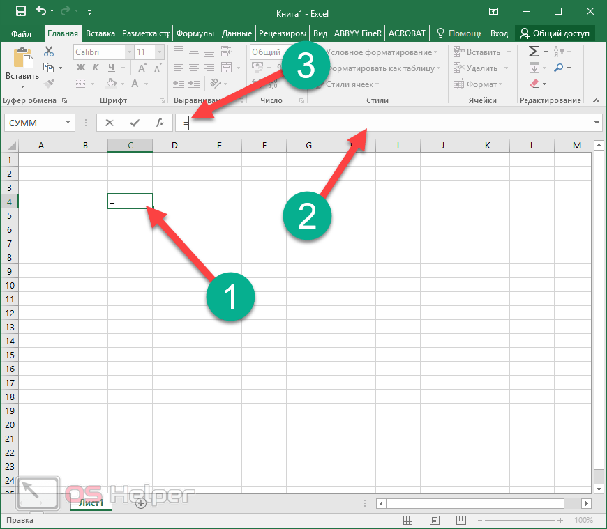
- Введите любое выражение. Использовать можно как цифры,
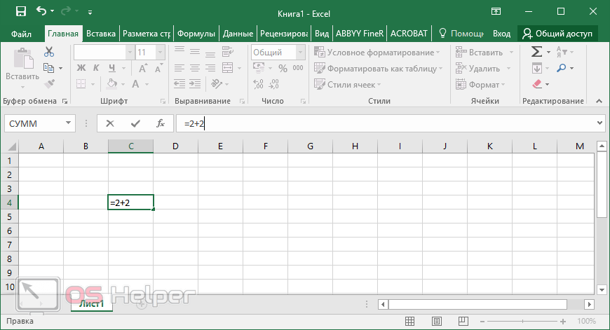
так и ссылки на ячейки.
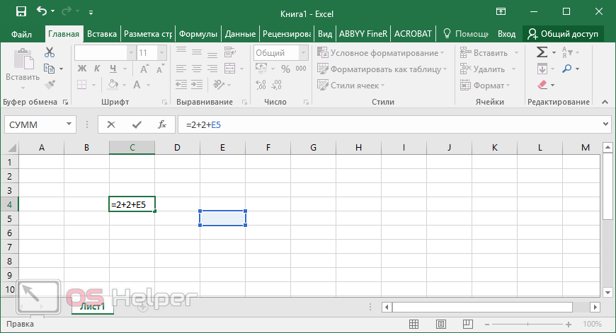
При этом затронутые ячейки всегда подсвечиваются. Это делается для того, чтобы вы не ошиблись с выбором. Визуально увидеть ошибку проще, чем в текстовом виде.
Из чего состоит формула
В качестве примера приведём следующее выражение.
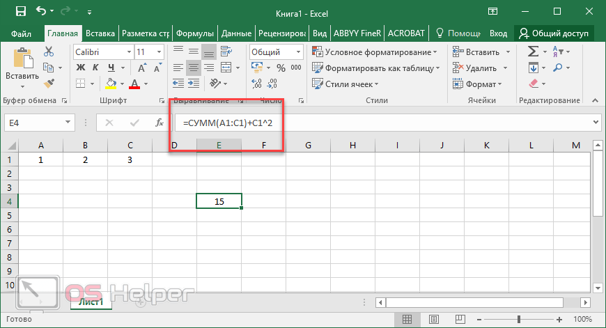
Оно состоит из:
- символ «=» – с него начинается любая формула;
- функция «СУММ»;
- аргумента функции «A1:C1» (в данном случае это массив ячеек с «A1» по «C1»);
- оператора «+» (сложение);
- ссылки на ячейку «C1»;
- оператора «^» (возведение в степень);
- константы «2».
Использование операторов
Операторы в редакторе Excel указывают какие именно операции нужно выполнить над указанными элементами формулы. При вычислении всегда соблюдается один и тот же порядок:
- скобки;
- экспоненты;
- умножение и деление (в зависимости от последовательности);
- сложение и вычитание (также в зависимости от последовательности).
Арифметические
К ним относятся:
- сложение – «+» (плюс);
[kod]=2+2[/kod]
- отрицание или вычитание – «-» (минус);
[kod]=2-2[/kod]
[kod]=-2[/kod]
Если перед числом поставить «минус», то оно примет отрицательное значение, но по модулю останется точно таким же.
- умножение – «*»;
[kod]=2*2[/kod]
- деление «/»;
[kod]=2/2[/kod]
- процент «%»;
[kod]=20%[/kod]
- возведение в степень – «^».
[kod]=2^2[/kod]
Операторы сравнения
Данные операторы применяются для сравнения значений. В результате операции возвращается ИСТИНА или ЛОЖЬ. К ним относятся:
- знак «равенства» – «=»;
[kod]=C1=D1[/kod]
- знак «больше» – «>»;
[kod]=C1>D1[/kod]
- знак «меньше» — «<»;
[kod]=C1<D1[/kod]
- знак «больше или равно» — «>=»;
[kod]=C1>=D1[/kod]
- знак «меньше или равно» — «<=»;
[kod]=C1<=D1[/kod]
- знак «не равно» — «<>».
[kod]=C1<>D1[/kod]
Оператор объединения текста
Для этой цели используется специальный символ «&» (амперсанд). При помощи его можно соединить различные фрагменты в одно целое – тот же принцип, что и с функцией «СЦЕПИТЬ». Приведем несколько примеров:
- Если вы хотите объединить текст в ячейках, то нужно использовать следующий код.
[kod]=A1&A2&A3[/kod]
- Для того чтобы вставить между ними какой-нибудь символ или букву, нужно использовать следующую конструкцию.
[kod]=A1&»,»&A2&»,»&A3[/kod]
- Объединять можно не только ячейки, но и обычные символы.
[kod]=»Авто»&»мобиль»[/kod]
Любой текст, кроме ссылок, необходимо указывать в кавычках. Иначе формула выдаст ошибку.
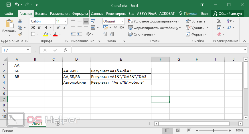
Обратите внимание, что кавычки используют именно такие, как на скриншоте.
Операторы ссылок
Для определения ссылок можно использовать следующие операторы:
- для того чтобы создать простую ссылку на нужный диапазон ячеек, достаточно указать первую и последнюю клетку этой области, а между ними символ «:»;
- для объединения ссылок используется знак «;»;
- если необходимо определить клетки, которые находятся на пересечении нескольких диапазонов, то между ссылками ставится «пробел». В данном случае выведется значение клетки «C7».
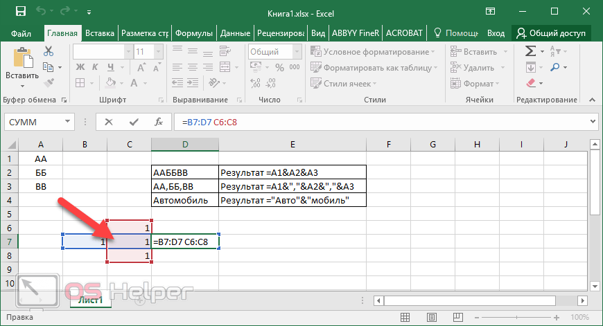
Поскольку только она попадает под определение «пересечения множеств». Именно такое название носит данный оператор (пробел).
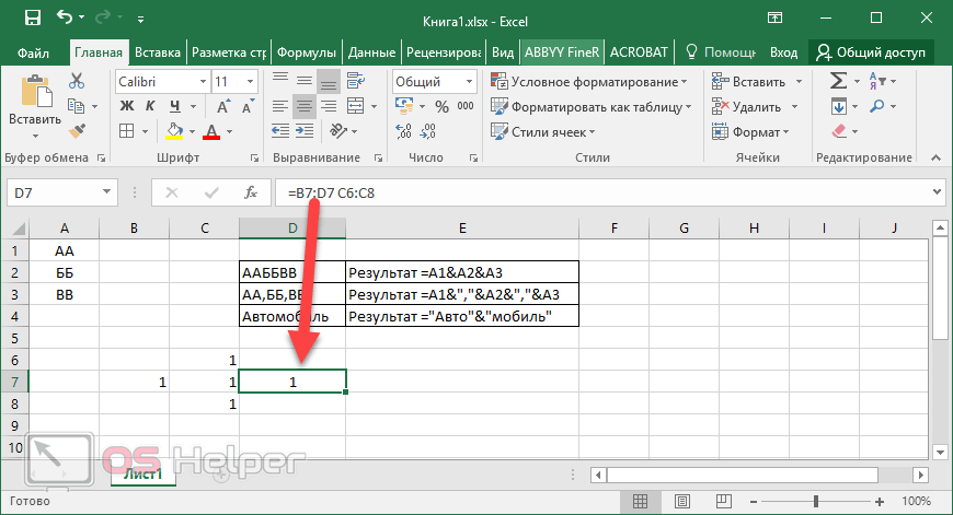
Давайте разберем ссылки более детально, поскольку это очень важный фрагмент в формулах.
Использование ссылок
Во время работы в редакторе Excel можно использовать ссылки различных видов. При этом большинство начинающих пользователей умеют пользоваться только самыми простыми из них. Мы вас научим, как правильно вводить ссылки всех форматов.
Простые ссылки A1
Как правило, данный вид используют чаще всего, поскольку их составлять намного удобнее, чем остальные.
В таких ссылках буквы означают столбец, а цифра – строку. Максимально можно задать:
- столбцов – от A до XFD (не больше 16384);
- строк – от 1 до 1048576.
Приведем несколько примеров:
- ячейка на пересечении строки 5 и столбца B – «B5»;
- диапазон ячеек в столбце B начиная с 5 по 25 строку – «B5:B25»;
- диапазон ячеек в строке 5 начиная со столбца B до F – «B5:F5»;
- все ячейки в строке 10 – «10:10»;
- все ячейки в строках с 10 по 15 – «10:15»;
- все клетки в столбце B – «B:B»;
- все клетки в столбцах с B по K – «B:K»;
- диапазон ячеек с B2 по F5 – «B2-F5».
Каждый раз при написании ссылки вы будете видеть вот такое выделение.
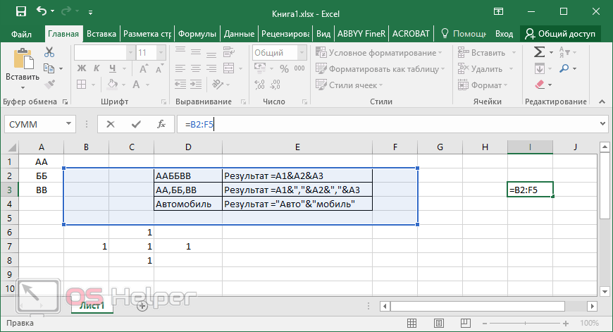
Ссылки на другой лист
Иногда в формулах используется информация с других листов. Работает это следующим образом.
[kod]=СУММ(Лист2!A5:C5)[/kod]
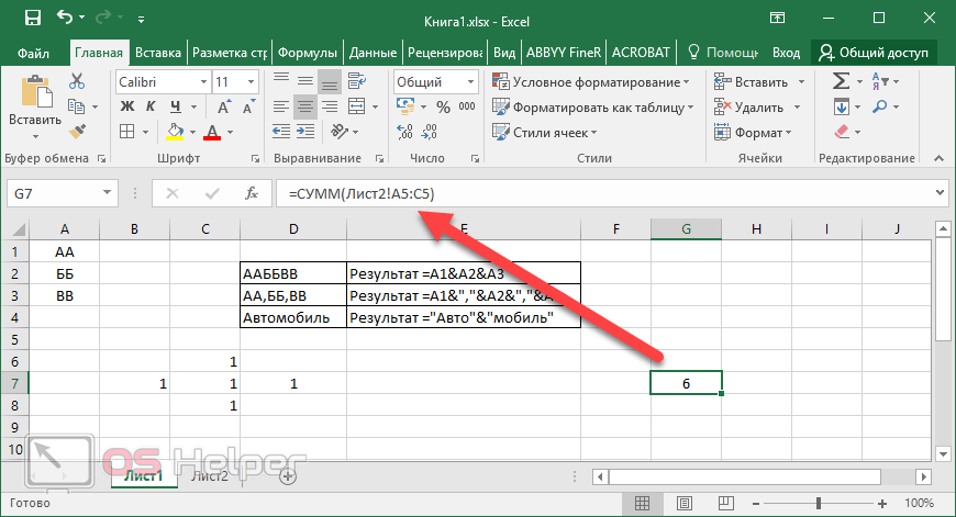
На втором листе указаны следующие данные.
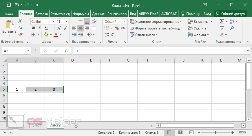
Если в названии листа есть пробел, то в формуле его нужно указывать в одинарных кавычках (апострофы).
[kod]=СУММ(‘Лист номер 2’!A5:C5)[/kod]
Абсолютные и относительные ссылки
Редактор Эксель работает с тремя видами ссылок:
- абсолютные;
- относительные;
- смешанные.
Рассмотрим их более внимательно.
Относительные ссылки
Все указанные ранее примеры принадлежат к относительному адресу ячеек. Данный тип самый популярный. Главное практическое преимущество в том, что редактор во время переноса изменит ссылки на другое значение. В соответствии с тем, куда именно вы скопировали эту формулу. Для подсчета будет учитываться количество клеток между старым и новым положением.
Представьте, что вам нужно растянуть эту формулу на всю колонку или строку. Вы же не будете вручную изменять буквы и цифры в адресах ячеек. Работает это следующим образом.
- Введём формулу для расчета суммы первой колонки.
[kod]=СУММ(B4:B9)[/kod]

- Нажмите на горячие клавиши [knopka]Ctrl[/knopka]+[knopka]C[/knopka]. Для того чтобы перенести формулу на соседнюю клетку, необходимо перейти туда и нажать на [knopka]Ctrl[/knopka]+[knopka]V[/knopka].
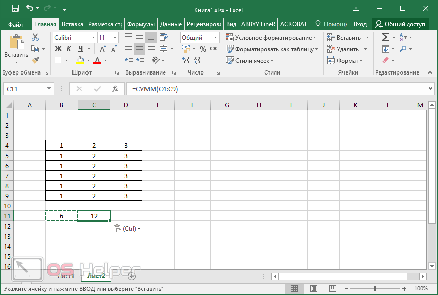
Если таблица очень большая, лучше кликнуть на правый нижний угол и, не отпуская пальца, протянуть указатель до конца. Если данных мало, то копировать при помощи горячих клавиш намного быстрее.
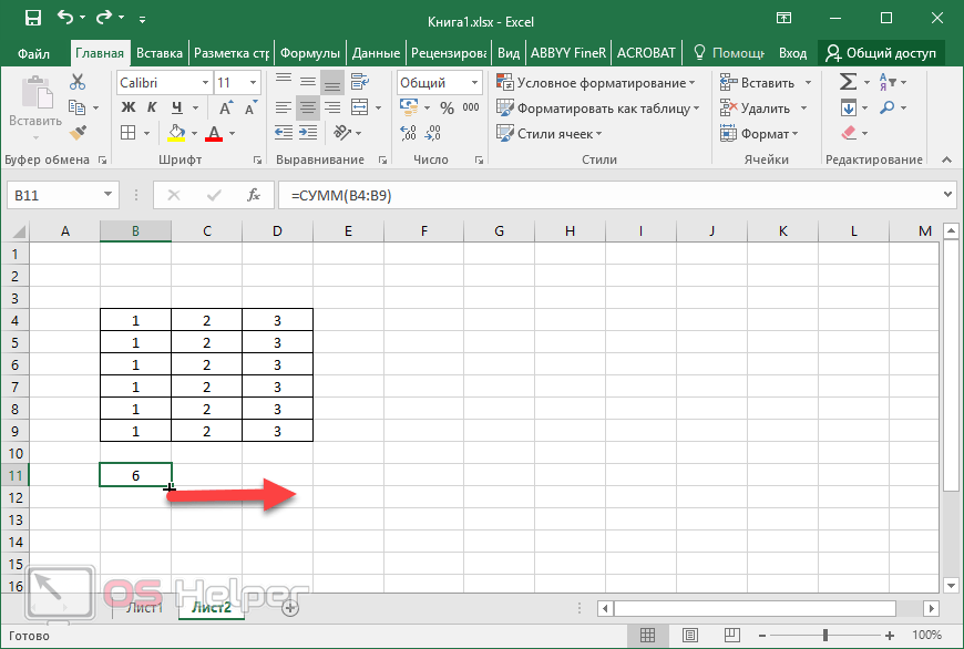
- Теперь посмотрите на новые формулы. Изменение индекса столбца произошло автоматически.
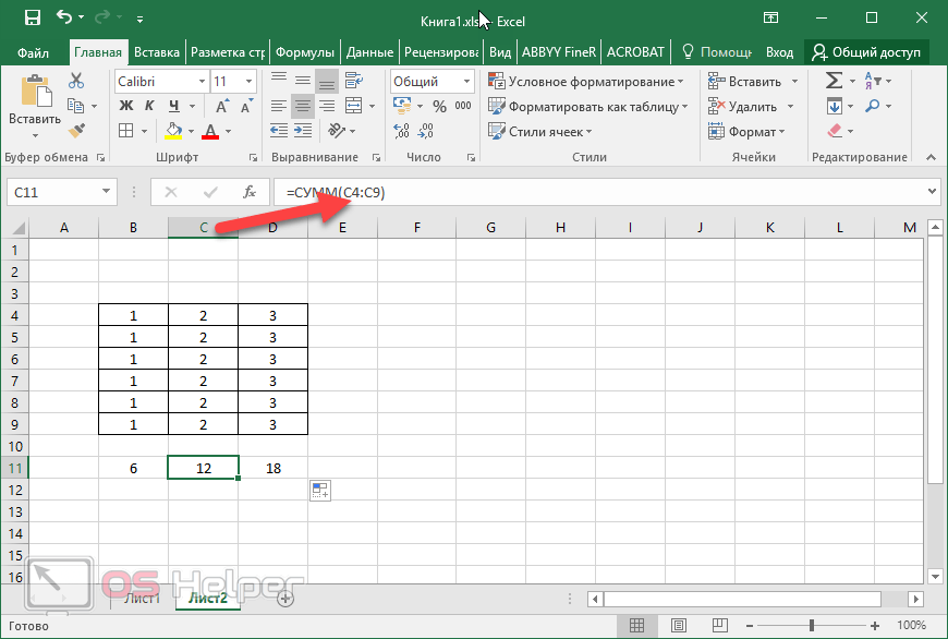
Абсолютные ссылки
Если вы хотите, чтобы при переносе формул все ссылки сохранялись (то есть чтобы они не менялись в автоматическом режиме), нужно использовать абсолютные адреса. Они указываются в виде «$B$2».
Если в ссылке перед цифрой или буквой указан знак доллара, то это значение не меняется. В качестве примера изменим вышеуказанную формулу на следующий вид.
[kod]=СУММ($B$4:$B$9)[/kod]
В итоге мы видим, что изменений никаких не произошло. Во всех столбцах у нас отображается одно и то же число.
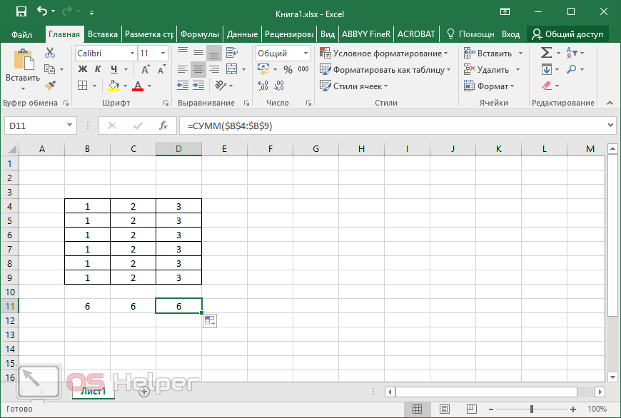
Смешанные ссылки
Данный тип адресов используется тогда, когда необходимо зафиксировать только столбец или строку, а не всё одновременно. Использовать можно следующие конструкции:
- $D1, $F5, $G3 – для фиксации столбцов;
- D$1, F$5, G$3 – для фиксации строк.
Работают с такими формулами только тогда, когда это необходимо. Например, если вам нужно работать с одной постоянной строкой данных, но при этом изменять только столбцы. И самое главное – если вы собираетесь рассчитать результат в разных ячейках, которые не расположены вдоль одной линии.
Дело в том, что когда вы скопируете формулу на другую строку, то в ссылках цифры автоматически изменятся на количество клеток от исходного значения. Если использовать смешанные адреса, то всё останется на месте. Делается это следующим образом.
- В качестве примера используем следующее выражение.
[kod]=B$4[/kod]
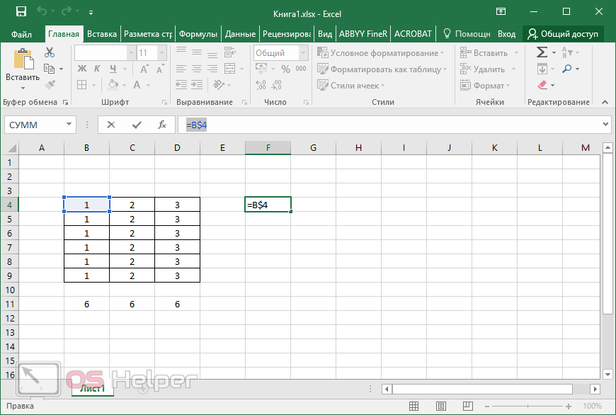
- Перенесем эту формулу в другую ячейку. Желательно не на следующую и на другой строке. Теперь вы видим, что новое выражение содержит ту же строчку (4), но другую букву, поскольку только она была относительной.
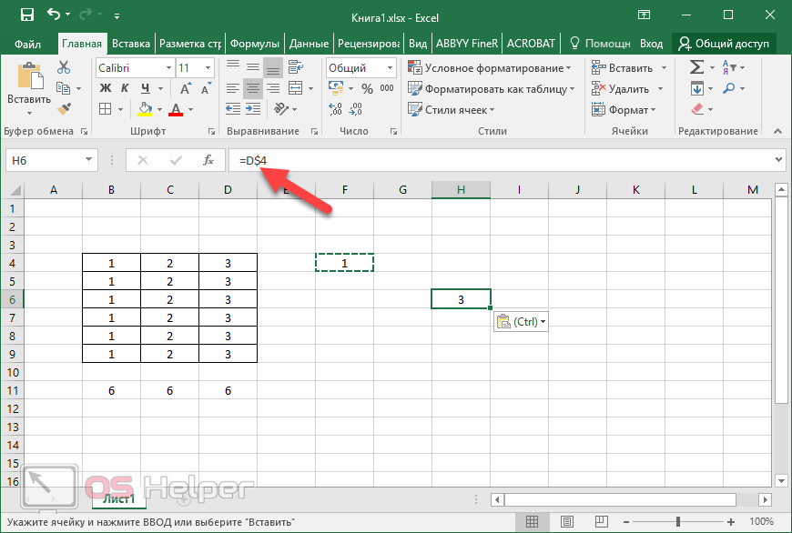
Трёхмерные ссылки
Под понятие «трёхмерные» попадают те адреса, в которых указывается диапазон листов. Пример формулы выглядит следующим образом.
[kod]=СУММ(Лист1:Лист4!A5)[/kod]
В данном случае результат будет соответствовать сумме всех ячеек «A5» на всех листах, начиная с 1 по 4. При составлении таких выражений необходимо придерживаться следующих условий:
- в массивах нельзя использовать подобные ссылки;
- трехмерные выражения запрещается использовать там, где есть пересечение ячеек (например, оператор «пробел»);
- при создании формул с трехмерными адресами можно использовать следующие функции: СРЗНАЧ, СТАНДОТКЛОНА, СТАНДОТКЛОН.В, СРЗНАЧА, СТАНДОТКЛОНПА, СТАНДОТКЛОН.Г, СУММ, СЧЁТЗ, СЧЁТ, МИН, МАКС, МИНА, МАКСА, ДИСПР, ПРОИЗВЕД, ДИСППА, ДИСП.В и ДИСПА.
Если нарушить эти правила, то вы увидите какую-нибудь ошибку.
Ссылки формата R1C1
Данный тип ссылок от «A1» отличается тем, что номер задается не только строкам, но и столбцам. Разработчики решили заменить обычный вид на этот вариант для удобства в макросах, но их можно использовать где угодно. Приведем несколько примеров таких адресов:
- R10C10 – абсолютная ссылка на клетку, которая расположена на десятой строке десятого столбца;
- R – абсолютная ссылка на текущую (в которой указывается формула) ссылку;
- R[-2] – относительная ссылка на строчку, которая расположена на две позиции выше этой;
- R[-3]C – относительная ссылка на клетку, которая расположена на три позиции выше в текущем столбце (где вы решили прописать формулу);
- R[5]C[5] – относительная ссылка на клетку, которая распложена на пять клеток правее и пять строк ниже текущей.
Использование имён
Программа Excel для обозначения диапазонов ячеек, одиночных ячеек, таблиц (обычные и сводные), констант и выражений позволяет создавать свои уникальные имена. При этом для редактора никакой разницы при работе с формулами нет – он понимает всё.
Имена вы можете использовать для умножения, деления, сложения, вычитания, расчета процентов, коэффициентов, отклонения, округления, НДС, ипотеки, кредита, сметы, табелей, различных бланков, скидки, зарплаты, стажа, аннуитетного платежа, работы с формулами «ВПР», «ВСД», «ПРОМЕЖУТОЧНЫЕ.ИТОГИ» и так далее. То есть можете делать, что угодно.
Главным условием можно назвать только одно – вы должны заранее определить это имя. Иначе Эксель о нём ничего знать не будет. Делается это следующим образом.
- Выделите какой-нибудь столбец.
- Вызовите контекстное меню.
- Выберите пункт «Присвоить имя».
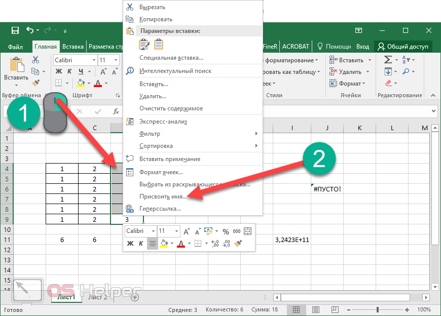
- Укажите желаемое имя этого объекта. При этом нужно придерживаться следующих правил.

- Для сохранения нажмите на кнопку «OK».
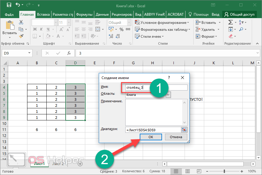
Точно так же можно присвоить имя какой-нибудь ячейке, тексту или числу.
Использовать информацию в таблице можно как при помощи имён, так и при помощи обычных ссылок. Так выглядит стандартный вариант.
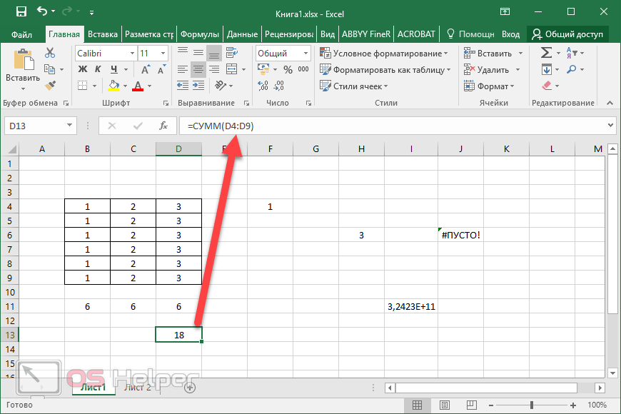
А если попробовать вместо адреса «D4:D9» вставить наше имя, то вы увидите подсказку. Достаточно написать несколько знаков, и вы увидите, что подходит (из базы имён) больше всего.
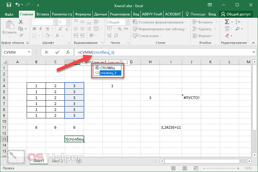
В нашем случае всё просто – «столбец_3». А представьте, что у вас таких имён будет большое множество. Все наизусть вы запомнить не сможете.
Использование функций
В редакторе Excel вставить функцию можно несколькими способами:
- вручную;
- при помощи панели инструментов;
- при помощи окна «Вставка функции».
Рассмотрим каждый метод более внимательно.
Ручной ввод
В этом случае всё просто – вы при помощи рук, собственных знаний и умений вводите формулы в специальной строке или прямо в ячейке.
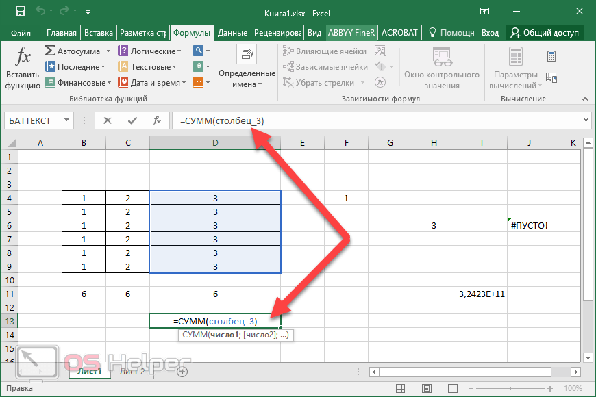
Если же у вас нет рабочего опыта в этой области, то лучше поначалу использовать более облегченные методы.
Панель инструментов
В этом случае необходимо:
- Перейти на вкладку «Формулы».
- Кликнуть на какую-нибудь библиотеку.
- Выбрать нужную функцию.
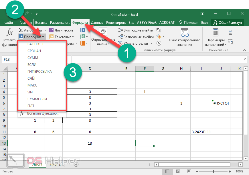
- Сразу после этого появится окно «Аргументы и функции» с уже выбранной функцией. Вам остается только проставить аргументы и сохранить формулу при помощи кнопки «OK».
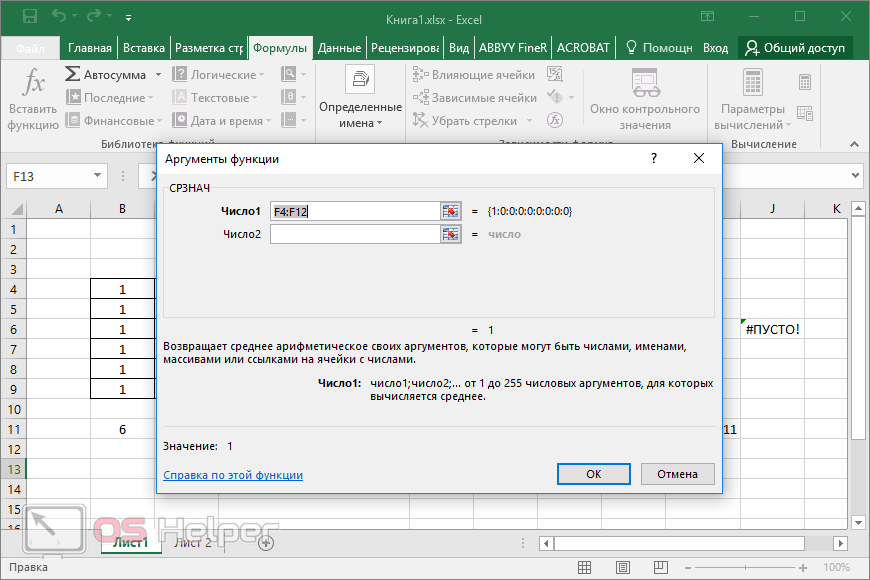
Мастер подстановки
Применить его можно следующим образом:
- Сделайте активной любую ячейку.
- Нажмите на иконку «Fx» или выполните сочетание клавиш [knopka]SHIFT[/knopka]+[knopka]F3[/knopka].
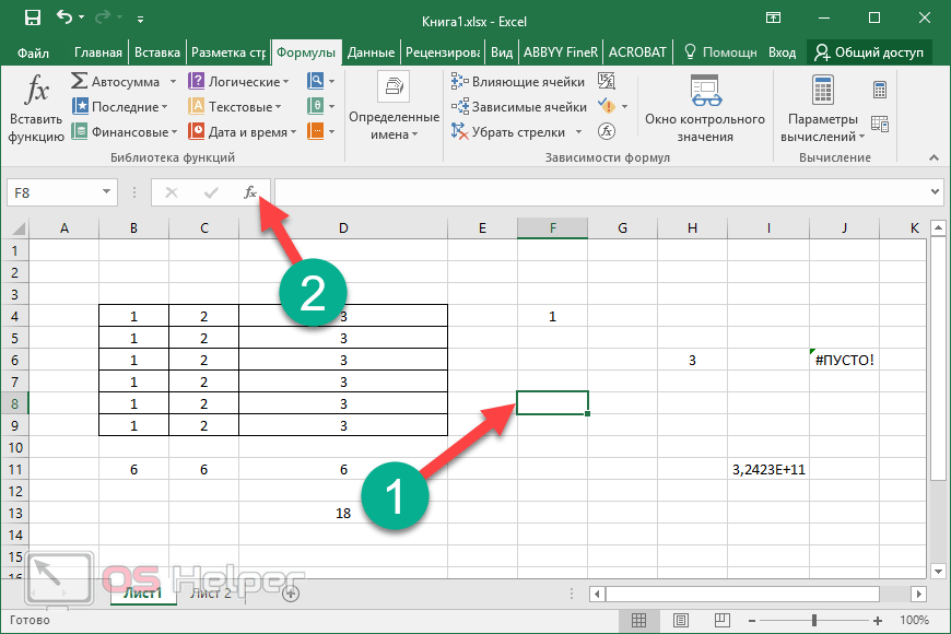
- Сразу после этого откроется окно «Вставка функции».
- Здесь вы увидите большой список различных функций, отсортированных по категориям. Кроме этого, можно воспользоваться поиском, если вы не можете найти нужный пункт.
Достаточно забить какое-нибудь слово, которым можно описать то, что вы хотите сделать, а редактор попробует вывести все подходящие варианты.
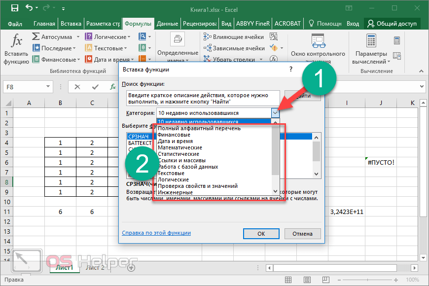
- Выберите какую-нибудь функцию из предложенного списка.
- Чтобы продолжить, нужно кликнуть на кнопку «OK».
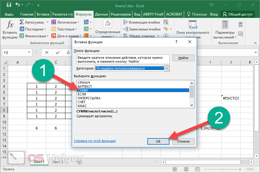
- Затем вас попросят указать «Аргументы и функции». Сделать это можно вручную либо просто выделить нужный диапазон ячеек.
- Для того чтобы применить все настройки, нужно нажать на кнопку «OK».
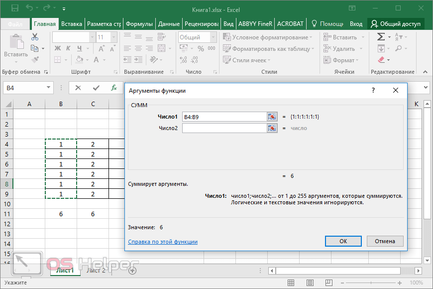
- В результате этого мы увидим цифру 6, хотя это было и так понятно, поскольку в окне «Аргументы и функции» выводится предварительный результат. Данные пересчитываются моментально при изменении любого из аргументов.
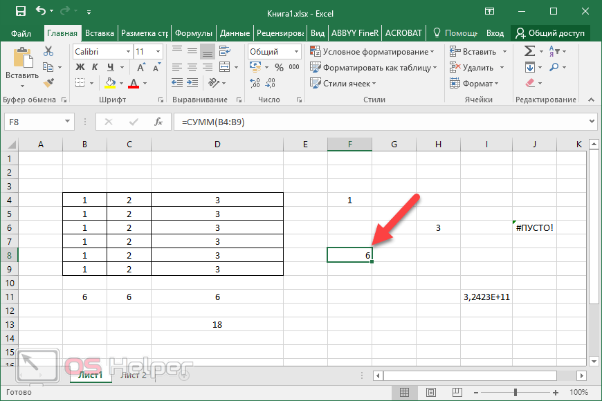
Использование вложенных функций
В качестве примера будем использовать формулы с логическими условиями. Для этого нам нужно будет добавить какую-нибудь таблицу.
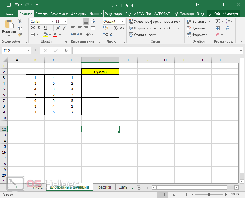
Затем придерживайтесь следующей инструкции:
- Кликните на первую ячейку. Вызовите окно «Вставка функции». Выберите функцию «Если». Для вставки нажмите на «OK».
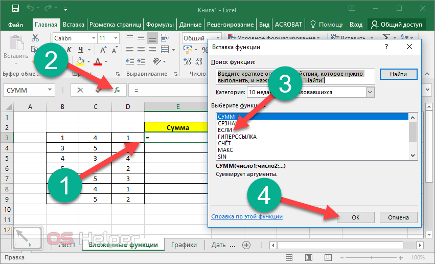
- Затем нужно будет составить какое-нибудь логическое выражение. Его необходимо записать в первое поле. Например, можно сложить значения трех ячеек в одной строке и проверить, будет ли сумма больше 10. В случае «истины» указываем текст «Больше 10». Для ложного результата – «Меньше 10». Затем для возврата в рабочее пространство нажимаем на «OK».
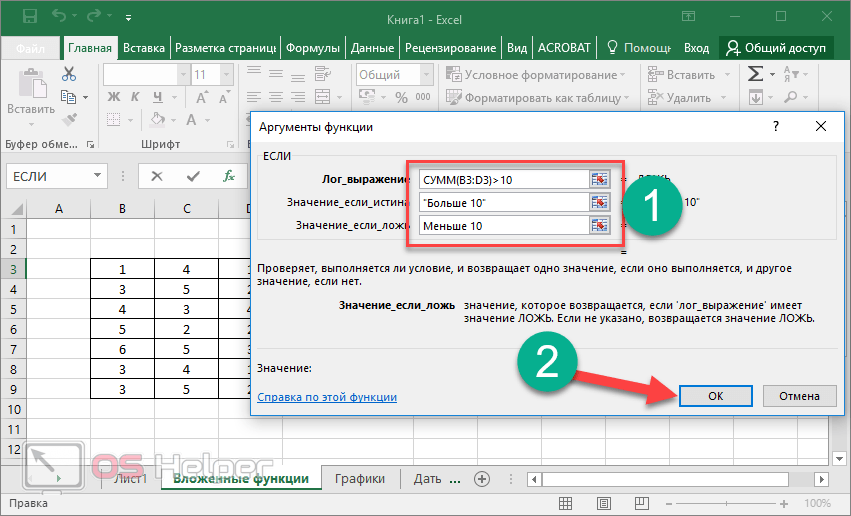
- В итоге мы видим следующее – редактор выдал, что сумма ячеек в третьей строке меньше 10. И это правильно. Значит, наш код работает.
[kod]=ЕСЛИ(СУММ(B3:D3)>10;»Больше 10″;»Меньше 10″)[/kod]
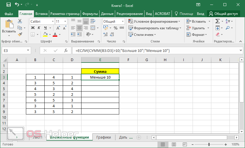
- Теперь нужно настроить и следующие клетки. В этом случае наша формула просто протягивается дальше. Для этого сначала необходимо навести курсор на правый нижний угол ячейки. После того как изменится курсор, нужно сделать левый клик и скопировать её до самого низа.
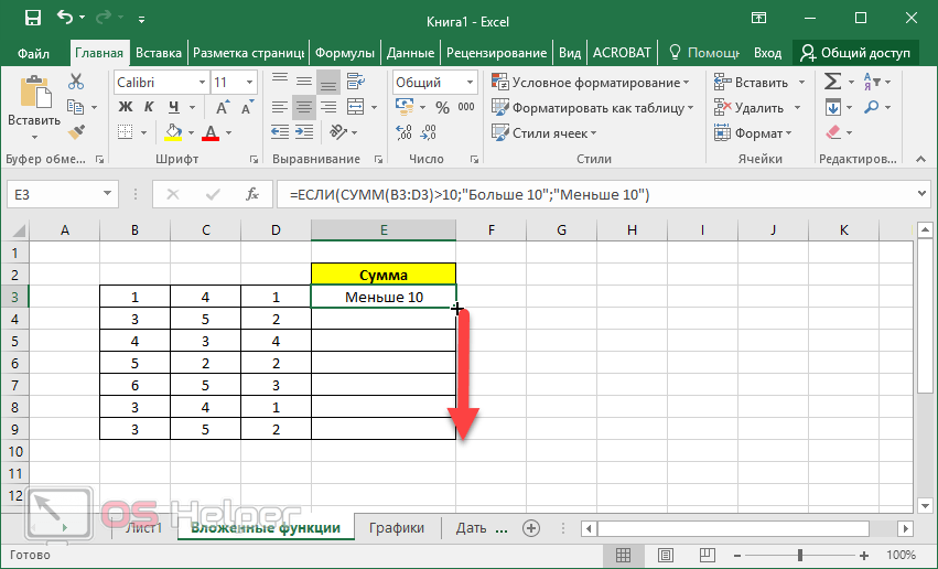
- В итоге редактор пересчитывает наше выражение для каждой строки.
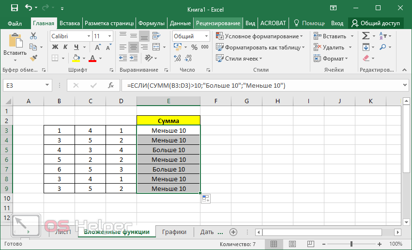
Как видите, копирование произошло весьма успешно, поскольку мы использовали относительные ссылки, о которых мы говорили ранее. Если же вам нужно закрепить адреса в аргументах функций, тогда используйте абсолютные значения.
Как редактировать формулу
Сделать это можно несколькими способами: использовать строку формул или специальный мастер. В первом случае всё просто – кликаете в специальное поле и вручную вводите нужные изменения. Но писать там не совсем удобно.
Единственное, что вы можете сделать, это увеличить поле для ввода. Для этого достаточно кликнуть на указанную иконку или нажать на сочетание клавиш [knopka]Ctrl[/knopka]+[knopka]Shift[/knopka]+[knopka]U[/knopka].
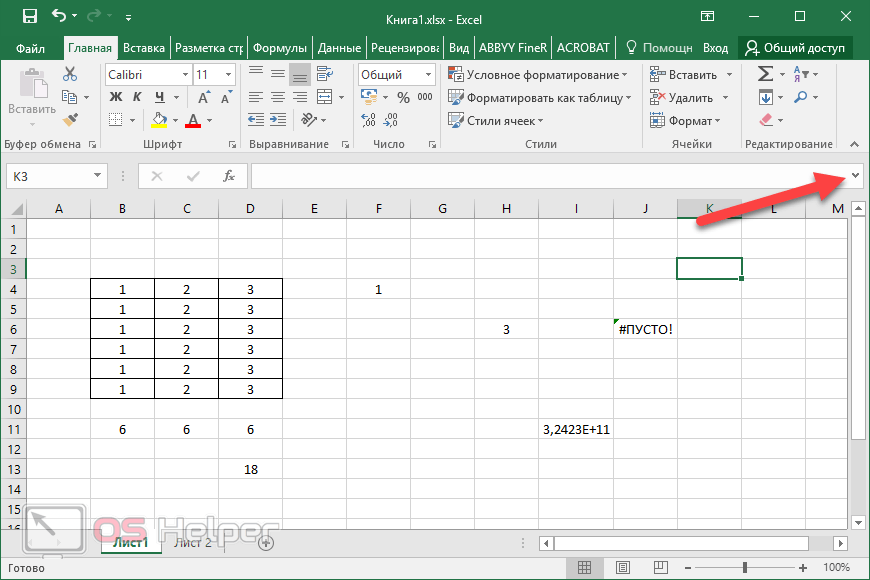
Стоит отметить, что это единственный способ, если вы не используете в формуле функции.
В случае использования функций всё становится намного проще. Для редактирования необходимо следовать следующей инструкции:
- Сделайте активной клетку с формулой. Нажмите на иконку «Fx».
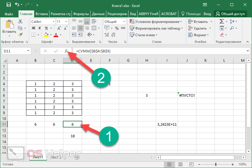
- После этого появится окно, в котором вы сможете в очень удобном виде изменить нужные вам аргументы функции. Кроме этого, здесь можно узнать, каким именно будет результат пересчета нового выражения.
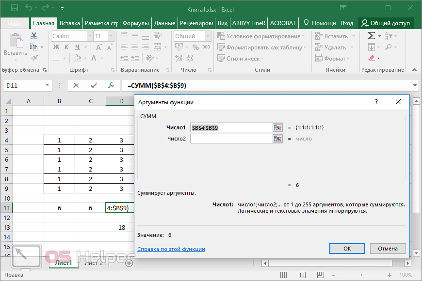
- Для сохранения внесенных изменений нужно использовать кнопку «OK».
Как убрать формулу
Для того чтобы удалить какое-нибудь выражение, достаточно сделать следующее:
- Кликните на любую ячейку.
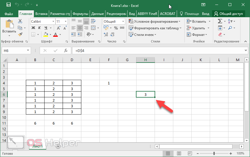
- Нажмите на кнопку [knopka]Delete[/knopka] или [knopka]Backspace[/knopka]. В результате этого клетка окажется пустой.
Добиться точно такого же результата можно и при помощи инструмента «Очистить всё».
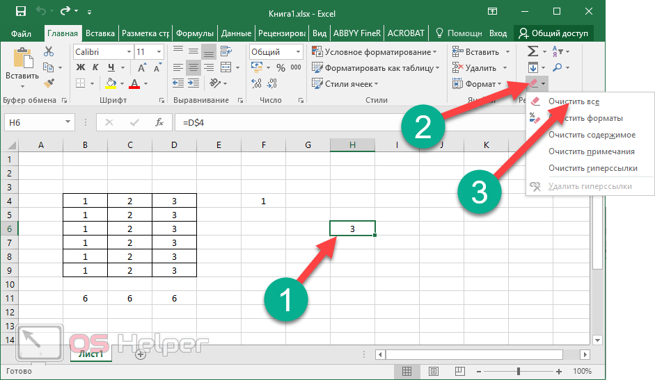
Возможные ошибки при составлении формул в редакторе Excel
Ниже перечислены самые популярные ошибки, которые допускаются пользователями:
- в выражении используется огромное количество вложенностей. Их должно быть не более 64;
- в формулах указываются пути к внешним книгам без полного пути;
- неправильно расставлены открывающиеся и закрывающиеся скобки. Именно поэтому в редакторе в строке формул все скобки подсвечиваются другим цветом;
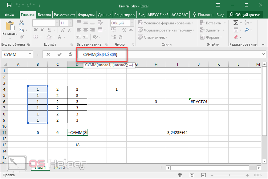
- имена книг и листов не берутся в кавычки;
- используются числа в неправильном формате. Например, если вам нужно указать $2000, необходимо вбить просто 2000 и выбрать соответствующий формат ячейки, поскольку символ $ задействован программой для абсолютных ссылок;
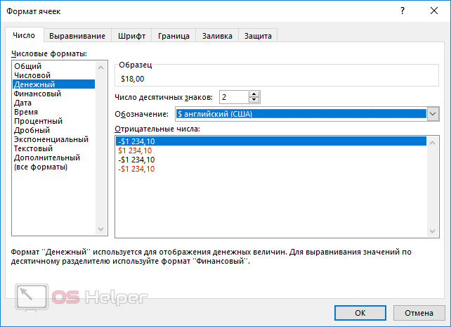
- не указываются обязательные аргументы функций. Обратите внимание на то, что необязательные аргументы указываются в квадратных скобках. Всё что без них – необходимо для полноценной работы формулы;
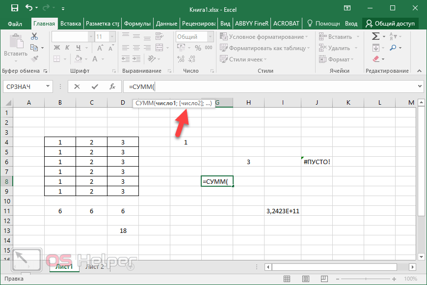
- неправильно указываются диапазоны ячеек. Для этого необходимо использовать оператор «:» (двоеточие).
Коды ошибок при работе с формулами
При работе с формулой вы можете увидеть следующие варианты ошибок:
- #ЗНАЧ! – данная ошибка показывает, что вы используете неправильный тип данных. Например, вместо числового значения пытаетесь использовать текст. Разумеется, Эксель не сможет вычислить сумму между двумя фразами;
- #ИМЯ? – подобная ошибка означает, что вы допустили опечатку в написании названия функции. Или же пытаетесь ввести что-то несуществующее. Так делать нельзя. Кроме этого, проблема может быть и в другом. Если вы уверены в имени функции, то попробуйте посмотреть на формулу более внимательно. Возможно, вы забыли какую-нибудь скобку. Кроме этого, нужно учитывать, что текстовые фрагменты указываются в кавычках. Если ничего не помогает, попробуйте составить выражение заново;
- #ЧИСЛО! – отображение подобного сообщения означает, что у вас какая-то проблема с аргументами или с результатом выполнения формулы. Например, число получилось слишком огромным или наоборот – маленьким;
- #ДЕЛ/0!– данная ошибка означает, что вы пытаетесь написать выражение, в котором происходит деление на ноль. Excel не может отменить правила математики. Поэтому такие действия здесь также запрещены;
- #Н/Д! – редактор может показать это сообщение, если какое-нибудь значение недоступно. Например, если вы используете функции ПОИСК, ПОИСКА, ПОИСКПОЗ, и Excel не нашел искомый фрагмент. Или же данных вообще нет и формуле не с чем работать;
- Если вы пытаетесь что-то посчитать, и программа Excel пишет слово #ССЫЛКА!, значит, в аргументе функции используется неправильный диапазон ячеек;
- #ПУСТО! – эта ошибка появляется в том случае, если у вас используется несогласующаяся формула с пересекающимися диапазонами. Точнее – если в действительности подобные ячейки отсутствуют (которые оказываются на пересечении двух диапазонов). Довольно часто такая ошибка возникает случайно. Достаточно оставить один пробел в аргументе, и редактор воспримет его как специальный оператор (о нём мы рассказывали ранее).
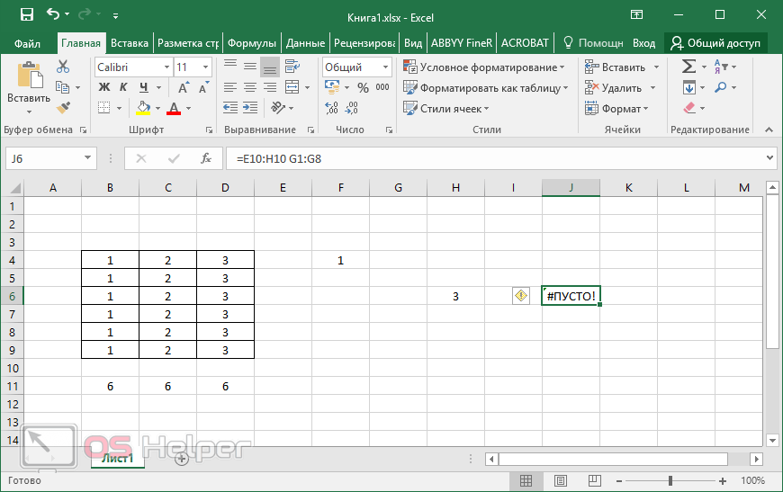
При редактировании формулы (ячейки подсвечиваются) вы увидите, что они на самом деле не пересекаются.
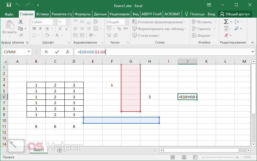
Иногда можно увидеть много символов #, которые полностью заполняют ячейку по ширине. На самом деле тут ошибки нет. Это означает, что вы работаете с числами, которые не помещаются в данную клетку.
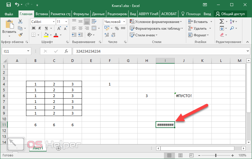
Для того чтобы увидеть содержащееся там значение, достаточно изменить размер столбца.

Кроме этого, можно использовать форматирование ячеек. Для этого необходимо выполнить несколько простых шагов:
- Вызовите контекстное меню. Выберите пункт «Формат ячеек».
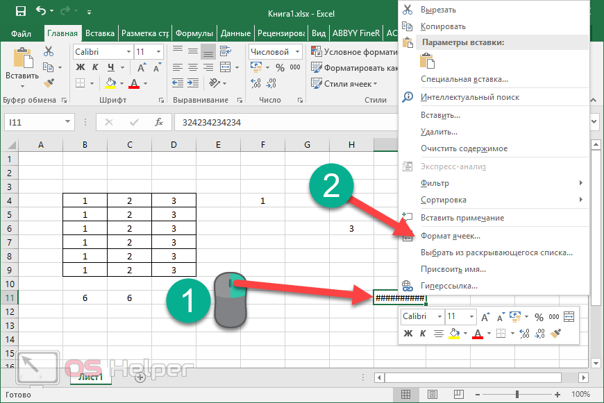
- Укажите тип «Общий». Для продолжения используйте кнопку «OK».
Благодаря этому редактор Эксель сможет перевести это число в другой формат, который умещается в данном столбце.
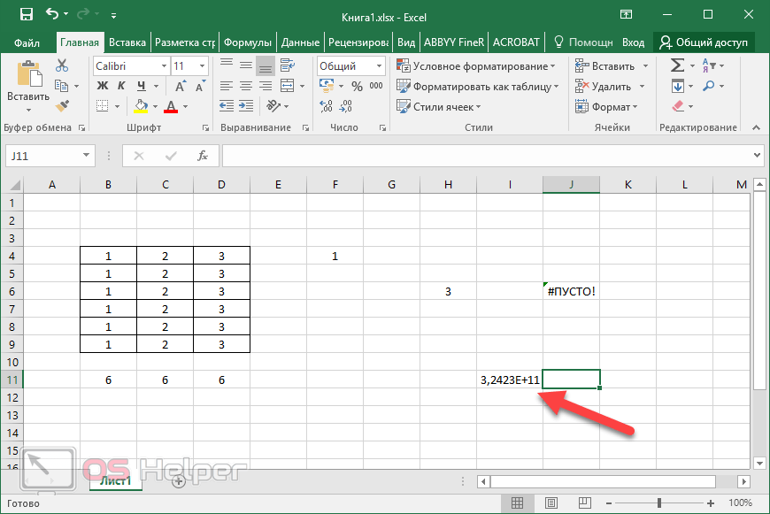
Примеры использования формул
Редактор Microsoft Excel позволяет обрабатывать информацию любым удобным для вас способом. Для этого есть все необходимые условия и возможности. Рассмотрим несколько примеров формул по категориям. Так вам будет проще разобраться.
Арифметика
Для того чтобы оценить математические возможности Экселя, нужно выполнить следующие действия.
- Создайте таблицу с какими-нибудь условными данными.

- Для того чтобы высчитать сумму, введите следующую формулу. Если хотите прибавить только одно значение, можно использовать оператор сложения («+»).
[kod]=СУММ(B3:C3)[/kod]
- Как ни странно, в редакторе Excel нельзя отнять при помощи функций. Для вычета используется обычный оператор «-». В этом случае код получится следующий.
[kod]=B3-C3[/kod]
- Для того чтобы определить, сколько первое число составляет от второго в процентах, нужно использовать вот такую простую конструкцию. Если вы захотите вычесть несколько значений, то придется прописывать «минус» для каждой ячейки.
[kod]=B3/C3%[/kod]
Обратите внимание, что символ процента ставится в конце, а не в начале. Кроме этого, при работе с процентами не нужно дополнительно умножать на 100. Это происходит автоматически.
- Для определения среднего значения используйте следующую формулу.
[kod]=СРЗНАЧ(B3:C3)[/kod]
- В результате описанных выше выражений, вы увидите следующий итог.
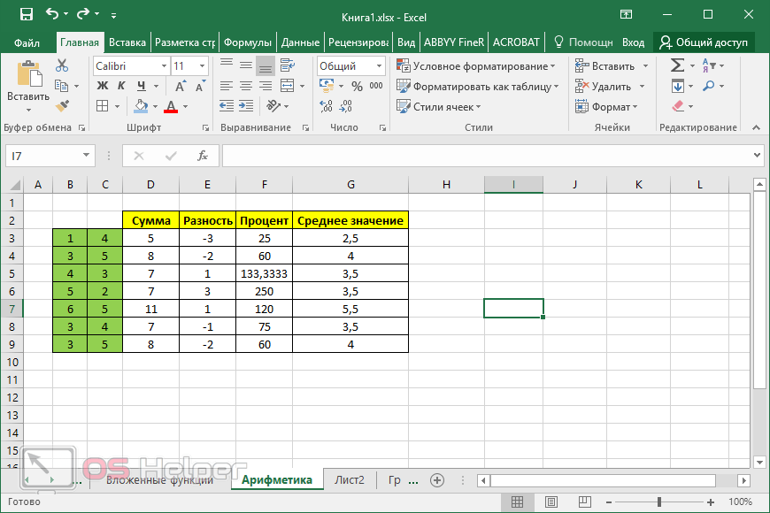
Условия
Считать ячейки можно с учетом определенных условий.
- Для этого увеличим нашу таблицу.
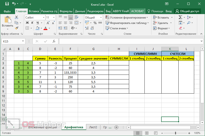
- Например, сложим те ячейки, у которых значение больше трёх.
[kod]=СУММЕСЛИ(B3;»>3″;B3:C3)[/kod]
- Excel может складывать с учетом сразу нескольких условий. Можно посчитать сумму клеток первого столбца, значение которых больше 2 и меньше 6. И ту же самую формулу можно установить для второй колонки.
[kod]=СУММЕСЛИМН(B3:B9;B3:B9;»>2″;B3:B9;»<6″)[/kod]
[kod]=СУММЕСЛИМН(C3:C9;C3:C9;»>2″;C3:C9;»<6″)[/kod]
- Также можно посчитать количество элементов, которые удовлетворяют какому-то условию. Например, пусть Эксель посчитает, сколько у нас чисел больше 3.
[kod]=СЧЁТЕСЛИ(B3:B9;»>3″)[/kod]
[kod]=СЧЁТЕСЛИ(C3:C9;»>3″)[/kod]
- Результат всех формул получится следующим.
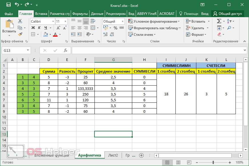
Математические функции и графики
При помощи Экселя можно рассчитывать различные функции и строить по ним графики, а затем проводить графический анализ. Как правило, подобные приёмы используются в презентациях.
В качестве примера попробуем построить графики для экспоненты и какого-нибудь уравнения. Инструкция будет следующей:
- Создадим таблицу. В первой графе у нас будет исходное число «X», во второй – функция «EXP», в третьей – указанное соотношение. Можно было бы сделать квадратичное выражение, но тогда бы результирующее значение на фоне экспоненты на графике практически пропало бы.
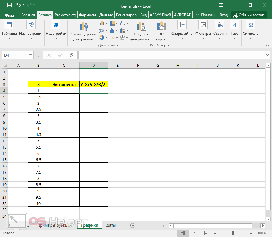
- Для того чтобы преобразовать значение «X», нужно указать следующие формулы.
[kod]=EXP(B4)[/kod]
[kod]=B4+5*B4^3/2[/kod]
- Дублируем эти выражения до самого конца. В итоге получаем следующий результат.
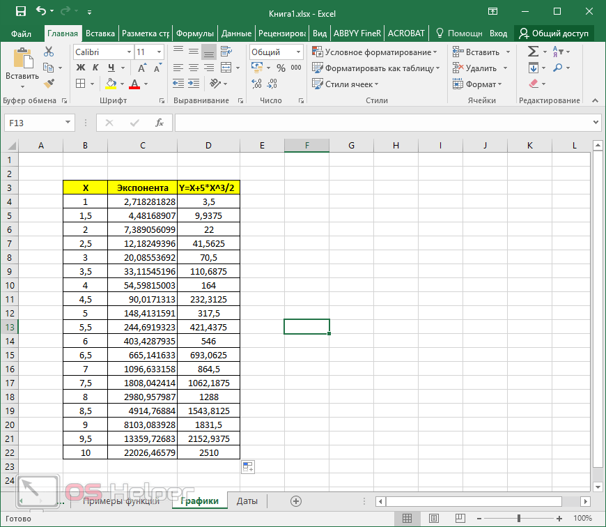
- Выделяем всю таблицу. Переходим на вкладку «Вставка». Кликаем на инструмент «Рекомендуемые диаграммы».
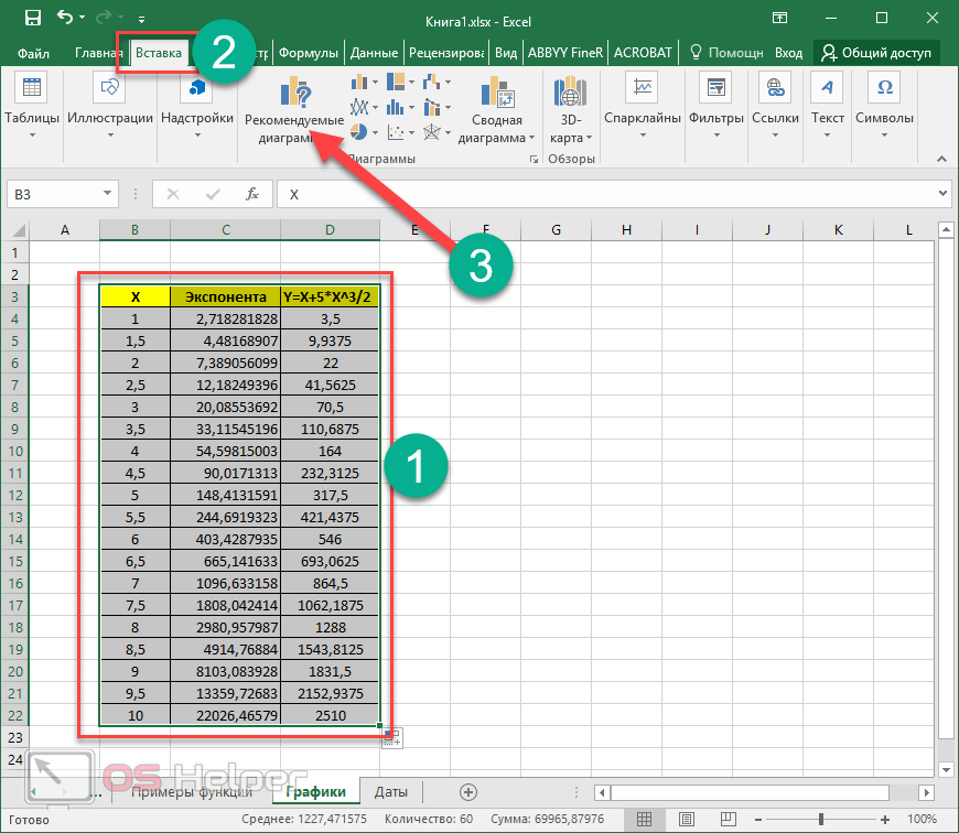
- Выбираем тип «Линия». Для продолжения кликаем на «OK».
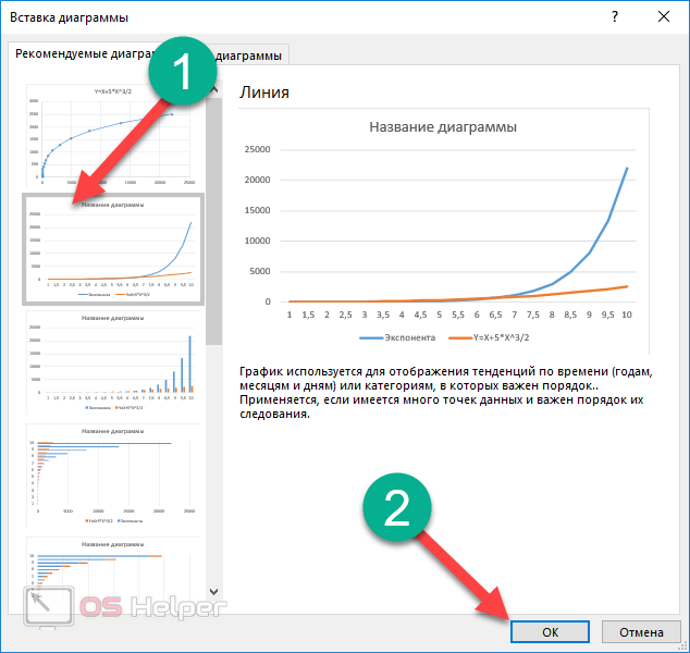
- Результат получился довольно-таки красивый и аккуратный.
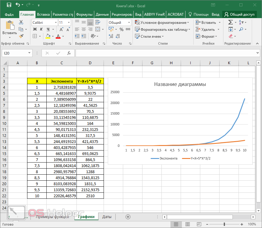
Как мы и говорили ранее, прирост экспоненты происходит намного быстрее, чем у обычного кубического уравнения.
Подобным образом можно представить графически любую функцию или математическое выражение.
Отличие в версиях MS Excel
Всё описанное выше подходит для современных программ 2007, 2010, 2013 и 2016 года. Старый редактор Эксель значительно уступает в плане возможностей, количества функций и инструментов. Если откроете официальную справку от Microsoft, то увидите, что они дополнительно указывают, в какой именно версии программы появилась данная функция.
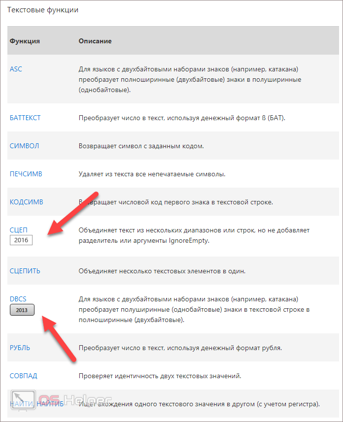
Во всём остальном всё выглядит практически точно так же. В качестве примера, посчитаем сумму нескольких ячеек. Для этого необходимо:
- Указать какие-нибудь данные для вычисления. Кликните на любую клетку. Нажмите на иконку «Fx».
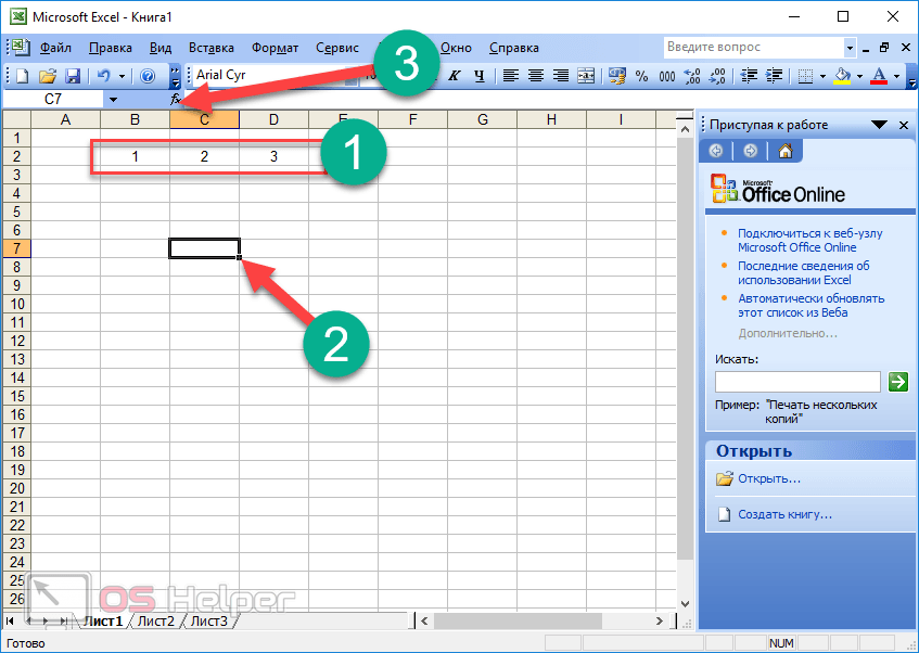
- Выбираем категорию «Математические». Находим функцию «СУММ» и нажимаем на «OK».
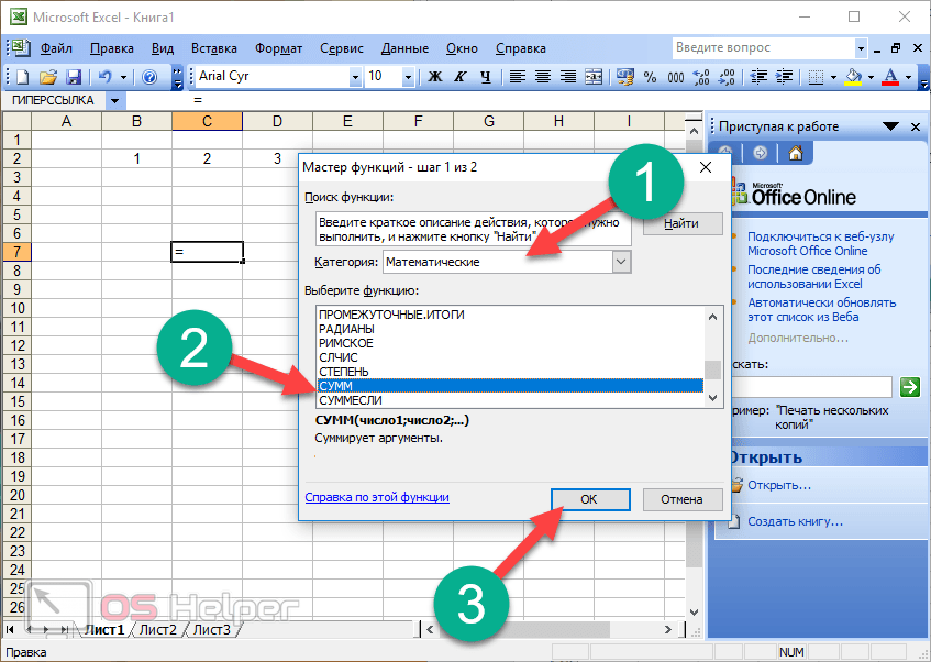
- Указываем данные в нужном диапазоне. Для того чтобы отобразить результат, нужно нажать на «OK».
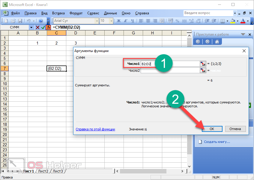
- Можете попробовать пересчитать в любом другом редакторе. Процесс будет происходить точно так же.
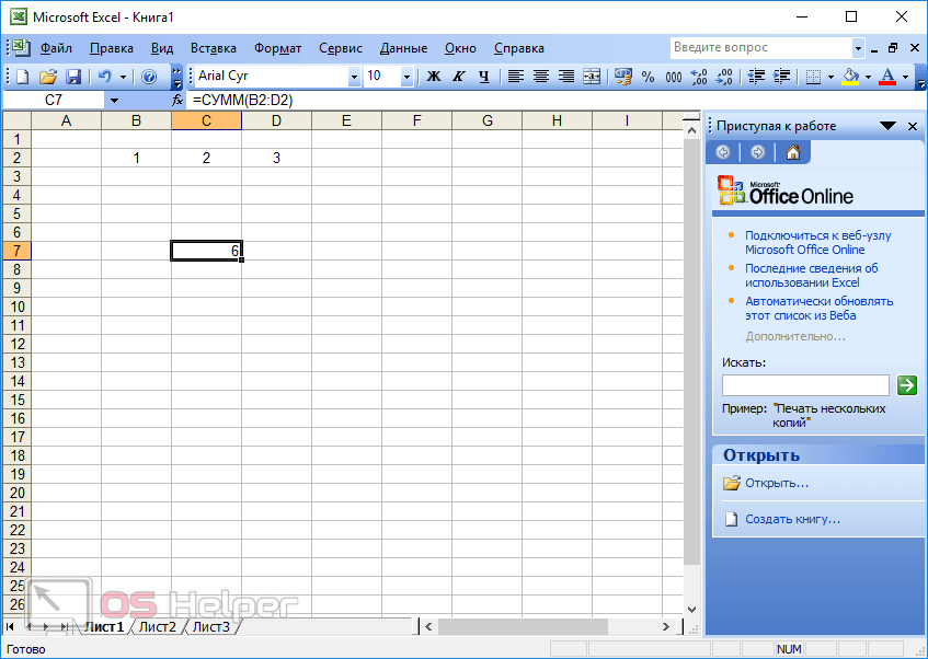
Заключение
В данном самоучителе мы рассказали обо всем, что связано с формулами в редакторе Excel, – от самого простого до очень сложного. Каждый раздел сопровождался подробными примерами и пояснениями. Это сделано для того, чтобы информация была доступной даже для полных чайников.
Если у вас что-то не получается, значит, вы допускаете где-то ошибку. Возможно, у вас есть опечатки в выражениях или же указаны неправильные ссылки на ячейки. Главное понять, что всё нужно вбивать очень аккуратно и внимательно. Тем более все функции не на английском, а на русском языке.
Кроме этого, важно помнить, что формулы должны начинаться с символа «=» (равно). Многие начинающие пользователи забывают про это.
Файл примеров
Для того чтобы вам было легче разобраться с описанными ранее формулами, мы подготовили специальный демо-файл, в котором составлялись все указанные примеры. Вы можете скачать его с нашего сайта совершенно бесплатно. Если во время обучения вы будете использовать готовую таблицу с формулами на основании заполненных данных, то добьетесь результата намного быстрее.
Видеоинструкция
Если наше описание вам не помогло, попробуйте посмотреть приложенное ниже видео, в котором рассказываются основные моменты более детально. Возможно, вы делаете всё правильно, но что-то упускаете из виду. С помощью этого ролика вы должны разобраться со всеми проблемами. Надеемся, что подобные уроки вам помогли. Заглядывайте к нам чаще.