
|
Function |
Description |
|---|---|
|
AVEDEV function |
Returns the average of the absolute deviations of data points from their mean |
|
AVERAGE function |
Returns the average of its arguments |
|
AVERAGEA function |
Returns the average of its arguments, including numbers, text, and logical values |
|
AVERAGEIF function |
Returns the average (arithmetic mean) of all the cells in a range that meet a given criteria |
|
AVERAGEIFS function |
Returns the average (arithmetic mean) of all cells that meet multiple criteria |
|
BETA.DIST function |
Returns the beta cumulative distribution function |
|
BETA.INV function |
Returns the inverse of the cumulative distribution function for a specified beta distribution |
|
BINOM.DIST function |
Returns the individual term binomial distribution probability |
|
BINOM.DIST.RANGE function |
Returns the probability of a trial result using a binomial distribution |
|
BINOM.INV function |
Returns the smallest value for which the cumulative binomial distribution is less than or equal to a criterion value |
|
CHISQ.DIST function |
Returns the cumulative beta probability density function |
|
CHISQ.DIST.RT function |
Returns the one-tailed probability of the chi-squared distribution |
|
CHISQ.INV function |
Returns the cumulative beta probability density function |
|
CHISQ.INV.RT function |
Returns the inverse of the one-tailed probability of the chi-squared distribution |
|
CHISQ.TEST function |
Returns the test for independence |
|
CONFIDENCE.NORM function |
Returns the confidence interval for a population mean |
|
CONFIDENCE.T function |
Returns the confidence interval for a population mean, using a Student’s t distribution |
|
CORREL function |
Returns the correlation coefficient between two data sets |
|
COUNT function |
Counts how many numbers are in the list of arguments |
|
COUNTA function |
Counts how many values are in the list of arguments |
|
COUNTBLANK function |
Counts the number of blank cells within a range |
|
COUNTIF function |
Counts the number of cells within a range that meet the given criteria |
|
COUNTIFS function |
Counts the number of cells within a range that meet multiple criteria |
|
COVARIANCE.P function |
Returns covariance, the average of the products of paired deviations |
|
COVARIANCE.S function |
Returns the sample covariance, the average of the products deviations for each data point pair in two data sets |
|
DEVSQ function |
Returns the sum of squares of deviations |
|
EXPON.DIST function |
Returns the exponential distribution |
|
F.DIST function |
Returns the F probability distribution |
|
F.DIST.RT function |
Returns the F probability distribution |
|
F.INV function |
Returns the inverse of the F probability distribution |
|
F.INV.RT function |
Returns the inverse of the F probability distribution |
|
F.TEST function |
Returns the result of an F-test |
|
FISHER function |
Returns the Fisher transformation |
|
FISHERINV function |
Returns the inverse of the Fisher transformation |
|
FORECAST function |
Returns a value along a linear trend Note: In Excel 2016, this function is replaced with FORECAST.LINEAR as part of the new Forecasting functions, but it’s still available for compatibility with earlier versions. |
|
FORECAST.ETS function |
Returns a future value based on existing (historical) values by using the AAA version of the Exponential Smoothing (ETS) algorithm |
|
FORECAST.ETS.CONFINT function |
Returns a confidence interval for the forecast value at the specified target date |
|
FORECAST.ETS.SEASONALITY function |
Returns the length of the repetitive pattern Excel detects for the specified time series |
|
FORECAST.ETS.STAT function |
Returns a statistical value as a result of time series forecasting |
|
FORECAST.LINEAR function |
Returns a future value based on existing values |
|
FREQUENCY function |
Returns a frequency distribution as a vertical array |
|
GAMMA function |
Returns the Gamma function value |
|
GAMMA.DIST function |
Returns the gamma distribution |
|
GAMMA.INV function |
Returns the inverse of the gamma cumulative distribution |
|
GAMMALN function |
Returns the natural logarithm of the gamma function, Γ(x) |
|
GAMMALN.PRECISE function |
Returns the natural logarithm of the gamma function, Γ(x) |
|
GAUSS function |
Returns 0.5 less than the standard normal cumulative distribution |
|
GEOMEAN function |
Returns the geometric mean |
|
GROWTH function |
Returns values along an exponential trend |
|
HARMEAN function |
Returns the harmonic mean |
|
HYPGEOM.DIST function |
Returns the hypergeometric distribution |
|
INTERCEPT function |
Returns the intercept of the linear regression line |
|
KURT function |
Returns the kurtosis of a data set |
|
LARGE function |
Returns the k-th largest value in a data set |
|
LINEST function |
Returns the parameters of a linear trend |
|
LOGEST function |
Returns the parameters of an exponential trend |
|
LOGNORM.DIST function |
Returns the cumulative lognormal distribution |
|
LOGNORM.INV function |
Returns the inverse of the lognormal cumulative distribution |
|
MAX function |
Returns the maximum value in a list of arguments |
|
MAXA function |
Returns the maximum value in a list of arguments, including numbers, text, and logical values |
|
MAXIFS function |
Returns the maximum value among cells specified by a given set of conditions or criteria |
|
MEDIAN function |
Returns the median of the given numbers |
|
MIN function |
Returns the minimum value in a list of arguments |
|
MINA function |
Returns the smallest value in a list of arguments, including numbers, text, and logical values |
|
MINIFS function |
Returns the minimum value among cells specified by a given set of conditions or criteria. |
|
MODE.MULT function |
Returns a vertical array of the most frequently occurring, or repetitive values in an array or range of data |
|
MODE.SNGL function |
Returns the most common value in a data set |
|
NEGBINOM.DIST function |
Returns the negative binomial distribution |
|
NORM.DIST function |
Returns the normal cumulative distribution |
|
NORM.INV function |
Returns the inverse of the normal cumulative distribution |
|
NORM.S.DIST function |
Returns the standard normal cumulative distribution |
|
NORM.S.INV function |
Returns the inverse of the standard normal cumulative distribution |
|
PEARSON function |
Returns the Pearson product moment correlation coefficient |
|
PERCENTILE.EXC function |
Returns the k-th percentile of values in a range, where k is in the range 0..1, exclusive |
|
PERCENTILE.INC function |
Returns the k-th percentile of values in a range |
|
PERCENTRANK.EXC function |
Returns the rank of a value in a data set as a percentage (0..1, exclusive) of the data set |
|
PERCENTRANK.INC function |
Returns the percentage rank of a value in a data set |
|
PERMUT function |
Returns the number of permutations for a given number of objects |
|
PERMUTATIONA function |
Returns the number of permutations for a given number of objects (with repetitions) that can be selected from the total objects |
|
PHI function |
Returns the value of the density function for a standard normal distribution |
|
POISSON.DIST function |
Returns the Poisson distribution |
|
PROB function |
Returns the probability that values in a range are between two limits |
|
QUARTILE.EXC function |
Returns the quartile of the data set, based on percentile values from 0..1, exclusive |
|
QUARTILE.INC function |
Returns the quartile of a data set |
|
RANK.AVG function |
Returns the rank of a number in a list of numbers |
|
RANK.EQ function |
Returns the rank of a number in a list of numbers |
|
RSQ function |
Returns the square of the Pearson product moment correlation coefficient |
|
SKEW function |
Returns the skewness of a distribution |
|
SKEW.P function |
Returns the skewness of a distribution based on a population: a characterization of the degree of asymmetry of a distribution around its mean |
|
SLOPE function |
Returns the slope of the linear regression line |
|
SMALL function |
Returns the k-th smallest value in a data set |
|
STANDARDIZE function |
Returns a normalized value |
|
STDEV.P function |
Calculates standard deviation based on the entire population |
|
STDEV.S function |
Estimates standard deviation based on a sample |
|
STDEVA function |
Estimates standard deviation based on a sample, including numbers, text, and logical values |
|
STDEVPA function |
Calculates standard deviation based on the entire population, including numbers, text, and logical values |
|
STEYX function |
Returns the standard error of the predicted y-value for each x in the regression |
|
T.DIST function |
Returns the Percentage Points (probability) for the Student t-distribution |
|
T.DIST.2T function |
Returns the Percentage Points (probability) for the Student t-distribution |
|
T.DIST.RT function |
Returns the Student’s t-distribution |
|
T.INV function |
Returns the t-value of the Student’s t-distribution as a function of the probability and the degrees of freedom |
|
T.INV.2T function |
Returns the inverse of the Student’s t-distribution |
|
T.TEST function |
Returns the probability associated with a Student’s t-test |
|
TREND function |
Returns values along a linear trend |
|
TRIMMEAN function |
Returns the mean of the interior of a data set |
|
VAR.P function |
Calculates variance based on the entire population |
|
VAR.S function |
Estimates variance based on a sample |
|
VARA function |
Estimates variance based on a sample, including numbers, text, and logical values |
|
VARPA function |
Calculates variance based on the entire population, including numbers, text, and logical values |
|
WEIBULL.DIST function |
Returns the Weibull distribution |
|
Z.TEST function |
Returns the one-tailed probability-value of a z-test |
ABS function
Math and trigonometry: Returns the absolute value of a number
ACCRINT function
Financial: Returns the accrued interest for a security that pays periodic interest
ACCRINTM function
Financial: Returns the accrued interest for a security that pays interest at maturity
ACOS function
Math and trigonometry: Returns the arccosine of a number
ACOSH function
Math and trigonometry: Returns the inverse hyperbolic cosine of a number
ACOT function

Math and trigonometry: Returns the arccotangent of a number
ACOTH function
Math and trigonometry: Returns the hyperbolic arccotangent of a number
AGGREGATE function
Math and trigonometry: Returns an aggregate in a list or database
ADDRESS function
Lookup and reference: Returns a reference as text to a single cell in a worksheet
AMORDEGRC function
Financial: Returns the depreciation for each accounting period by using a depreciation coefficient
AMORLINC function
Financial: Returns the depreciation for each accounting period
AND function
Logical: Returns TRUE if all of its arguments are TRUE
ARABIC function
Math and trigonometry: Converts a Roman number to Arabic, as a number
AREAS function
Lookup and reference: Returns the number of areas in a reference
ARRAYTOTEXT function

Text: Returns an array of text values from any specified range
ASC function
Text: Changes full-width (double-byte) English letters or katakana within a character string to half-width (single-byte) characters
ASIN function
Math and trigonometry: Returns the arcsine of a number
ASINH function
Math and trigonometry: Returns the inverse hyperbolic sine of a number
ATAN function
Math and trigonometry: Returns the arctangent of a number
ATAN2 function
Math and trigonometry: Returns the arctangent from x- and y-coordinates
ATANH function
Math and trigonometry: Returns the inverse hyperbolic tangent of a number
AVEDEV function
Statistical: Returns the average of the absolute deviations of data points from their mean
AVERAGE function
Statistical: Returns the average of its arguments
AVERAGEA function
Statistical: Returns the average of its arguments, including numbers, text, and logical values
AVERAGEIF function
Statistical: Returns the average (arithmetic mean) of all the cells in a range that meet a given criteria
AVERAGEIFS function
Statistical: Returns the average (arithmetic mean) of all cells that meet multiple criteria.
BAHTTEXT function
Text: Converts a number to text, using the ß (baht) currency format
BASE function
Math and trigonometry: Converts a number into a text representation with the given radix (base)
BESSELI function
Engineering: Returns the modified Bessel function In(x)
BESSELJ function
Engineering: Returns the Bessel function Jn(x)
BESSELK function
Engineering: Returns the modified Bessel function Kn(x)
BESSELY function
Engineering: Returns the Bessel function Yn(x)
BETADIST function
Compatibility: Returns the beta cumulative distribution function
In Excel 2007, this is a Statistical function.
BETA.DIST function

Statistical: Returns the beta cumulative distribution function
BETAINV function
Compatibility: Returns the inverse of the cumulative distribution function for a specified beta distribution
In Excel 2007, this is a Statistical function.
BETA.INV function
Statistical: Returns the inverse of the cumulative distribution function for a specified beta distribution
BIN2DEC function
Engineering: Converts a binary number to decimal
BIN2HEX function
Engineering: Converts a binary number to hexadecimal
BIN2OCT function
Engineering: Converts a binary number to octal
BINOMDIST function
Compatibility: Returns the individual term binomial distribution probability
In Excel 2007, this is a Statistical function.
BINOM.DIST function
Statistical: Returns the individual term binomial distribution probability
BINOM.DIST.RANGE function
Statistical: Returns the probability of a trial result using a binomial distribution
BINOM.INV function
Statistical: Returns the smallest value for which the cumulative binomial distribution is less than or equal to a criterion value
BITAND function
Engineering: Returns a ‘Bitwise And’ of two numbers
BITLSHIFT function
Engineering: Returns a value number shifted left by shift_amount bits
BITOR function
Engineering: Returns a bitwise OR of 2 numbers
BITRSHIFT function
Engineering: Returns a value number shifted right by shift_amount bits
BITXOR function
Engineering: Returns a bitwise ‘Exclusive Or’ of two numbers
BYCOL
Logical: Applies a LAMBDA to each column and returns an array of the results
BYROW
Logical: Applies a LAMBDA to each row and returns an array of the results
CALL function
Add-in and Automation: Calls a procedure in a dynamic link library or code resource
CEILING function
Compatibility: Rounds a number to the nearest integer or to the nearest multiple of significance
CEILING.MATH function
Math and trigonometry: Rounds a number up, to the nearest integer or to the nearest multiple of significance
CEILING.PRECISE function
Math and trigonometry: Rounds a number the nearest integer or to the nearest multiple of significance. Regardless of the sign of the number, the number is rounded up.
CELL function
Information: Returns information about the formatting, location, or contents of a cell
This function is not available in Excel for the web.
CHAR function
Text: Returns the character specified by the code number
CHIDIST function
Compatibility: Returns the one-tailed probability of the chi-squared distribution
Note: In Excel 2007, this is a Statistical function.
CHIINV function
Compatibility: Returns the inverse of the one-tailed probability of the chi-squared distribution
Note: In Excel 2007, this is a Statistical function.
CHITEST function
Compatibility: Returns the test for independence
Note: In Excel 2007, this is a Statistical function.
CHISQ.DIST function
Statistical: Returns the cumulative beta probability density function
CHISQ.DIST.RT function
Statistical: Returns the one-tailed probability of the chi-squared distribution
CHISQ.INV function
Statistical: Returns the cumulative beta probability density function
CHISQ.INV.RT function
Statistical: Returns the inverse of the one-tailed probability of the chi-squared distribution
CHISQ.TEST function
Statistical: Returns the test for independence
CHOOSE function
Lookup and reference: Chooses a value from a list of values
CHOOSECOLS
Lookup and reference: Returns the specified columns from an array
CHOOSEROWS
Lookup and reference: Returns the specified rows from an array
CLEAN function
Text: Removes all nonprintable characters from text
CODE function
Text: Returns a numeric code for the first character in a text string
COLUMN function
Lookup and reference: Returns the column number of a reference
COLUMNS function
Lookup and reference: Returns the number of columns in a reference
COMBIN function
Math and trigonometry: Returns the number of combinations for a given number of objects
COMBINA function
Math and trigonometry:
Returns the number of combinations with repetitions for a given number of items
COMPLEX function
Engineering: Converts real and imaginary coefficients into a complex number
CONCAT function

Text: Combines the text from multiple ranges and/or strings, but it doesn’t provide the delimiter or IgnoreEmpty arguments.
CONCATENATE function
Text: Joins several text items into one text item
CONFIDENCE function
Compatibility: Returns the confidence interval for a population mean
In Excel 2007, this is a Statistical function.
CONFIDENCE.NORM function
Statistical: Returns the confidence interval for a population mean
CONFIDENCE.T function
Statistical: Returns the confidence interval for a population mean, using a Student’s t distribution
CONVERT function
Engineering: Converts a number from one measurement system to another
CORREL function
Statistical: Returns the correlation coefficient between two data sets
COS function
Math and trigonometry: Returns the cosine of a number
COSH function
Math and trigonometry: Returns the hyperbolic cosine of a number
COT function
Math and trigonometry: Returns the hyperbolic cosine of a number
COTH function
Math and trigonometry: Returns the cotangent of an angle
COUNT function
Statistical: Counts how many numbers are in the list of arguments
COUNTA function
Statistical: Counts how many values are in the list of arguments
COUNTBLANK function
Statistical: Counts the number of blank cells within a range
COUNTIF function
Statistical: Counts the number of cells within a range that meet the given criteria
COUNTIFS function
Statistical: Counts the number of cells within a range that meet multiple criteria
COUPDAYBS function
Financial: Returns the number of days from the beginning of the coupon period to the settlement date
COUPDAYS function
Financial: Returns the number of days in the coupon period that contains the settlement date
COUPDAYSNC function
Financial: Returns the number of days from the settlement date to the next coupon date
COUPNCD function
Financial: Returns the next coupon date after the settlement date
COUPNUM function
Financial: Returns the number of coupons payable between the settlement date and maturity date
COUPPCD function
Financial: Returns the previous coupon date before the settlement date
COVAR function
Compatibility: Returns covariance, the average of the products of paired deviations
In Excel 2007, this is a Statistical function.
COVARIANCE.P function
Statistical: Returns covariance, the average of the products of paired deviations
COVARIANCE.S function
Statistical: Returns the sample covariance, the average of the products deviations for each data point pair in two data sets
CRITBINOM function
Compatibility: Returns the smallest value for which the cumulative binomial distribution is less than or equal to a criterion value
In Excel 2007, this is a Statistical function.
CSC function
Math and trigonometry: Returns the cosecant of an angle
CSCH function
Math and trigonometry: Returns the hyperbolic cosecant of an angle
CUBEKPIMEMBER function
Cube: Returns a key performance indicator (KPI) name, property, and measure, and displays the name and property in the cell. A KPI is a quantifiable measurement, such as monthly gross profit or quarterly employee turnover, used to monitor an organization’s performance.
CUBEMEMBER function
Cube: Returns a member or tuple in a cube hierarchy. Use to validate that the member or tuple exists in the cube.
CUBEMEMBERPROPERTY function
Cube: Returns the value of a member property in the cube. Use to validate that a member name exists within the cube and to return the specified property for this member.
CUBERANKEDMEMBER function
Cube: Returns the nth, or ranked, member in a set. Use to return one or more elements in a set, such as the top sales performer or top 10 students.
CUBESET function
Cube: Defines a calculated set of members or tuples by sending a set expression to the cube on the server, which creates the set, and then returns that set to Microsoft Office Excel.
CUBESETCOUNT function
Cube: Returns the number of items in a set.
CUBEVALUE function
Cube: Returns an aggregated value from a cube.
CUMIPMT function
Financial: Returns the cumulative interest paid between two periods
CUMPRINC function
Financial: Returns the cumulative principal paid on a loan between two periods
DATE function
Date and time: Returns the serial number of a particular date
DATEDIF function
Date and time: Calculates the number of days, months, or years between two dates. This function is useful in formulas where you need to calculate an age.
DATEVALUE function
Date and time: Converts a date in the form of text to a serial number
DAVERAGE function
Database: Returns the average of selected database entries
DAY function
Date and time: Converts a serial number to a day of the month
DAYS function
Date and time: Returns the number of days between two dates
DAYS360 function
Date and time: Calculates the number of days between two dates based on a 360-day year
DB function
Financial: Returns the depreciation of an asset for a specified period by using the fixed-declining balance method
DBCS function
Text: Changes half-width (single-byte) English letters or katakana within a character string to full-width (double-byte) characters
DCOUNT function
Database: Counts the cells that contain numbers in a database
DCOUNTA function
Database: Counts nonblank cells in a database
DDB function
Financial: Returns the depreciation of an asset for a specified period by using the double-declining balance method or some other method that you specify
DEC2BIN function
Engineering: Converts a decimal number to binary
DEC2HEX function
Engineering: Converts a decimal number to hexadecimal
DEC2OCT function
Engineering: Converts a decimal number to octal
DECIMAL function
Math and trigonometry: Converts a text representation of a number in a given base into a decimal number
DEGREES function
Math and trigonometry: Converts radians to degrees
DELTA function
Engineering: Tests whether two values are equal
DEVSQ function
Statistical: Returns the sum of squares of deviations
DGET function
Database: Extracts from a database a single record that matches the specified criteria
DISC function
Financial: Returns the discount rate for a security
DMAX function
Database: Returns the maximum value from selected database entries
DMIN function
Database: Returns the minimum value from selected database entries
DOLLAR function
Text: Converts a number to text, using the $ (dollar) currency format
DOLLARDE function
Financial: Converts a dollar price, expressed as a fraction, into a dollar price, expressed as a decimal number
DOLLARFR function
Financial: Converts a dollar price, expressed as a decimal number, into a dollar price, expressed as a fraction
DPRODUCT function
Database: Multiplies the values in a particular field of records that match the criteria in a database
DROP
Lookup and reference: Excludes a specified number of rows or columns from the start or end of an array
DSTDEV function
Database: Estimates the standard deviation based on a sample of selected database entries
DSTDEVP function
Database: Calculates the standard deviation based on the entire population of selected database entries
DSUM function
Database: Adds the numbers in the field column of records in the database that match the criteria
DURATION function
Financial: Returns the annual duration of a security with periodic interest payments
DVAR function
Database: Estimates variance based on a sample from selected database entries
DVARP function
Database: Calculates variance based on the entire population of selected database entries
EDATE function
Date and time: Returns the serial number of the date that is the indicated number of months before or after the start date
EFFECT function
Financial: Returns the effective annual interest rate
ENCODEURL function
Web: Returns a URL-encoded string
This function is not available in Excel for the web.
EOMONTH function
Date and time: Returns the serial number of the last day of the month before or after a specified number of months
ERF function
Engineering: Returns the error function
ERF.PRECISE function
Engineering: Returns the error function
ERFC function
Engineering: Returns the complementary error function
ERFC.PRECISE function
Engineering: Returns the complementary ERF function integrated between x and infinity
ERROR.TYPE function
Information: Returns a number corresponding to an error type
EUROCONVERT function
Add-in and Automation: Converts a number to euros, converts a number from euros to a euro member currency, or converts a number from one euro member currency to another by using the euro as an intermediary (triangulation).
EVEN function
Math and trigonometry: Rounds a number up to the nearest even integer
EXACT function
Text: Checks to see if two text values are identical
EXP function
Math and trigonometry: Returns e raised to the power of a given number
EXPAND
Lookup and reference: Expands or pads an array to specified row and column dimensions
EXPON.DIST function
Statistical: Returns the exponential distribution
EXPONDIST function
Compatibility: Returns the exponential distribution
In Excel 2007, this is a Statistical function.
FACT function
Math and trigonometry: Returns the factorial of a number
FACTDOUBLE function
Math and trigonometry: Returns the double factorial of a number
FALSE function
Logical: Returns the logical value FALSE
F.DIST function
Statistical: Returns the F probability distribution
FDIST function
Compatibility: Returns the F probability distribution
In Excel 2007, this is a Statistical function.
F.DIST.RT function
Statistical: Returns the F probability distribution
FILTER function
Lookup and reference: Filters a range of data based on criteria you define
FILTERXML function
Web: Returns specific data from the XML content by using the specified XPath
This function is not available in Excel for the web.
FIND, FINDB functions
Text: Finds one text value within another (case-sensitive)
F.INV function
Statistical: Returns the inverse of the F probability distribution
F.INV.RT function
Statistical: Returns the inverse of the F probability distribution
FINV function
Compatibility: Returns the inverse of the F probability distribution
In Excel 2007this is a Statistical function.
FISHER function
Statistical: Returns the Fisher transformation
FISHERINV function
Statistical: Returns the inverse of the Fisher transformation
FIXED function
Text: Formats a number as text with a fixed number of decimals
FLOOR function
Compatibility: Rounds a number down, toward zero
In Excel 2007 and Excel 2010, this is a Math and trigonometry function.
FLOOR.MATH function
Math and trigonometry: Rounds a number down, to the nearest integer or to the nearest multiple of significance
FLOOR.PRECISE function
Math and trigonometry: Rounds a number the nearest integer or to the nearest multiple of significance. Regardless of the sign of the number, the number is rounded up.
FORECAST function
Statistical: Returns a value along a linear trend
In Excel 2016, this function is replaced with FORECAST.LINEAR as part of the new Forecasting functions, but it’s still available for compatibility with earlier versions.
FORECAST.ETS function

Statistical: Returns a future value based on existing (historical) values by using the AAA version of the Exponential Smoothing (ETS) algorithm
FORECAST.ETS.CONFINT function
Statistical: Returns a confidence interval for the forecast value at the specified target date
FORECAST.ETS.SEASONALITY function
Statistical: Returns the length of the repetitive pattern Excel detects for the specified time series
FORECAST.ETS.STAT function
Statistical: Returns a statistical value as a result of time series forecasting
FORECAST.LINEAR function
Statistical: Returns a future value based on existing values
FORMULATEXT function
Lookup and reference: Returns the formula at the given reference as text
FREQUENCY function
Statistical: Returns a frequency distribution as a vertical array
F.TEST function
Statistical: Returns the result of an F-test
FTEST function
Compatibility: Returns the result of an F-test
In Excel 2007, this is a Statistical function.
FV function
Financial: Returns the future value of an investment
FVSCHEDULE function
Financial: Returns the future value of an initial principal after applying a series of compound interest rates
GAMMA function
Statistical: Returns the Gamma function value
GAMMA.DIST function
Statistical: Returns the gamma distribution
GAMMADIST function
Compatibility: Returns the gamma distribution
In Excel 2007, this is a Statistical function.
GAMMA.INV function
Statistical: Returns the inverse of the gamma cumulative distribution
GAMMAINV function
Compatibility: Returns the inverse of the gamma cumulative distribution
In Excel 2007, this is a Statistical function.
GAMMALN function
Statistical: Returns the natural logarithm of the gamma function, Γ(x)
GAMMALN.PRECISE function
Statistical: Returns the natural logarithm of the gamma function, Γ(x)
GAUSS function
Statistical: Returns 0.5 less than the standard normal cumulative distribution
GCD function
Math and trigonometry: Returns the greatest common divisor
GEOMEAN function
Statistical: Returns the geometric mean
GESTEP function
Engineering: Tests whether a number is greater than a threshold value
GETPIVOTDATA function
Lookup and reference: Returns data stored in a PivotTable report
GROWTH function
Statistical: Returns values along an exponential trend
HARMEAN function
Statistical: Returns the harmonic mean
HEX2BIN function
Engineering: Converts a hexadecimal number to binary
HEX2DEC function
Engineering: Converts a hexadecimal number to decimal
HEX2OCT function
Engineering: Converts a hexadecimal number to octal
HLOOKUP function
Lookup and reference: Looks in the top row of an array and returns the value of the indicated cell
HOUR function
Date and time: Converts a serial number to an hour
HSTACK
Lookup and reference: Appends arrays horizontally and in sequence to return a larger array
HYPERLINK function
Lookup and reference: Creates a shortcut or jump that opens a document stored on a network server, an intranet, or the Internet
HYPGEOM.DIST function
Statistical: Returns the hypergeometric distribution
HYPGEOMDIST function
Compatibility: Returns the hypergeometric distribution
In Excel 2007, this is a Statistical function.
IF function
Logical: Specifies a logical test to perform
IFERROR function
Logical: Returns a value you specify if a formula evaluates to an error; otherwise, returns the result of the formula
IFNA function
Logical: Returns the value you specify if the expression resolves to #N/A, otherwise returns the result of the expression
IFS function
Logical: Checks whether one or more conditions are met and returns a value that corresponds to the first TRUE condition.
IMABS function
Engineering: Returns the absolute value (modulus) of a complex number
IMAGINARY function
Engineering: Returns the imaginary coefficient of a complex number
IMARGUMENT function
Engineering: Returns the argument theta, an angle expressed in radians
IMCONJUGATE function
Engineering: Returns the complex conjugate of a complex number
IMCOS function
Engineering: Returns the cosine of a complex number
IMCOSH function
Engineering: Returns the hyperbolic cosine of a complex number
IMCOT function
Engineering: Returns the cotangent of a complex number
IMCSC function
Engineering: Returns the cosecant of a complex number
IMCSCH function
Engineering: Returns the hyperbolic cosecant of a complex number
IMDIV function
Engineering: Returns the quotient of two complex numbers
IMEXP function
Engineering: Returns the exponential of a complex number
IMLN function
Engineering: Returns the natural logarithm of a complex number
IMLOG10 function
Engineering: Returns the base-10 logarithm of a complex number
IMLOG2 function
Engineering: Returns the base-2 logarithm of a complex number
IMPOWER function
Engineering: Returns a complex number raised to an integer power
IMPRODUCT function
Engineering: Returns the product of complex numbers
IMREAL function
Engineering: Returns the real coefficient of a complex number
IMSEC function
Engineering: Returns the secant of a complex number
IMSECH function
Engineering: Returns the hyperbolic secant of a complex number
IMSIN function
Engineering: Returns the sine of a complex number
IMSINH function
Engineering: Returns the hyperbolic sine of a complex number
IMSQRT function
Engineering: Returns the square root of a complex number
IMSUB function
Engineering: Returns the difference between two complex numbers
IMSUM function
Engineering: Returns the sum of complex numbers
IMTAN function
Engineering: Returns the tangent of a complex number
INDEX function
Lookup and reference: Uses an index to choose a value from a reference or array
INDIRECT function
Lookup and reference: Returns a reference indicated by a text value
INFO function
Information: Returns information about the current operating environment
This function is not available in Excel for the web.
INT function
Math and trigonometry: Rounds a number down to the nearest integer
INTERCEPT function
Statistical: Returns the intercept of the linear regression line
INTRATE function
Financial: Returns the interest rate for a fully invested security
IPMT function
Financial: Returns the interest payment for an investment for a given period
IRR function
Financial: Returns the internal rate of return for a series of cash flows
ISBLANK function
Information: Returns TRUE if the value is blank
ISERR function
Information: Returns TRUE if the value is any error value except #N/A
ISERROR function
Information: Returns TRUE if the value is any error value
ISEVEN function
Information: Returns TRUE if the number is even
ISFORMULA function
Information: Returns TRUE if there is a reference to a cell that contains a formula
ISLOGICAL function
Information: Returns TRUE if the value is a logical value
ISNA function
Information: Returns TRUE if the value is the #N/A error value
ISNONTEXT function
Information: Returns TRUE if the value is not text
ISNUMBER function
Information: Returns TRUE if the value is a number
ISODD function
Information: Returns TRUE if the number is odd
ISOMITTED
Information: Checks whether the value in a LAMBDA is missing and returns TRUE or FALSE
ISREF function
Information: Returns TRUE if the value is a reference
ISTEXT function
Information: Returns TRUE if the value is text
ISO.CEILING function
Math and trigonometry: Returns a number that is rounded up to the nearest integer or to the nearest multiple of significance
ISOWEEKNUM function
Date and time: Returns the number of the ISO week number of the year for a given date
ISPMT function
Financial: Calculates the interest paid during a specific period of an investment
JIS function
Text: Changes half-width (single-byte) characters within a string to full-width (double-byte) characters
KURT function
Statistical: Returns the kurtosis of a data set
LAMBDA
Logical: Create custom, reusable functions and call them by a friendly name
LARGE function
Statistical: Returns the k-th largest value in a data set
LCM function
Math and trigonometry: Returns the least common multiple
LEFT, LEFTB functions
Text: Returns the leftmost characters from a text value
LEN, LENB functions
Text: Returns the number of characters in a text string
LET
Logical: Assigns names to calculation results
LINEST function
Statistical: Returns the parameters of a linear trend
LN function
Math and trigonometry: Returns the natural logarithm of a number
LOG function
Math and trigonometry: Returns the logarithm of a number to a specified base
LOG10 function
Math and trigonometry: Returns the base-10 logarithm of a number
LOGEST function
Statistical: Returns the parameters of an exponential trend
LOGINV function
Compatibility: Returns the inverse of the lognormal cumulative distribution
LOGNORM.DIST function
Statistical: Returns the cumulative lognormal distribution
LOGNORMDIST function
Compatibility: Returns the cumulative lognormal distribution
LOGNORM.INV function
Statistical: Returns the inverse of the lognormal cumulative distribution
LOOKUP function
Lookup and reference: Looks up values in a vector or array
LOWER function
Text: Converts text to lowercase
MAKEARRAY
Logical: Returns a calculated array of a specified row and column size, by applying a LAMBDA
MAP
Logical: Returns an array formed by mapping each value in the array(s) to a new value by applying a LAMBDA to create a new value
MATCH function
Lookup and reference: Looks up values in a reference or array
MAX function
Statistical: Returns the maximum value in a list of arguments
MAXA function
Statistical: Returns the maximum value in a list of arguments, including numbers, text, and logical values
MAXIFS function
Statistical: Returns the maximum value among cells specified by a given set of conditions or criteria
MDETERM function
Math and trigonometry: Returns the matrix determinant of an array
MDURATION function
Financial: Returns the Macauley modified duration for a security with an assumed par value of $100
MEDIAN function
Statistical: Returns the median of the given numbers
MID, MIDB functions
Text: Returns a specific number of characters from a text string starting at the position you specify
MIN function
Statistical: Returns the minimum value in a list of arguments
MINIFS function
Statistical: Returns the minimum value among cells specified by a given set of conditions or criteria.
MINA function
Statistical: Returns the smallest value in a list of arguments, including numbers, text, and logical values
MINUTE function
Date and time: Converts a serial number to a minute
MINVERSE function
Math and trigonometry: Returns the matrix inverse of an array
MIRR function
Financial: Returns the internal rate of return where positive and negative cash flows are financed at different rates
MMULT function
Math and trigonometry: Returns the matrix product of two arrays
MOD function
Math and trigonometry: Returns the remainder from division
MODE function
Compatibility: Returns the most common value in a data set
In Excel 2007, this is a Statistical function.
MODE.MULT function
Statistical: Returns a vertical array of the most frequently occurring, or repetitive values in an array or range of data
MODE.SNGL function
Statistical: Returns the most common value in a data set
MONTH function
Date and time: Converts a serial number to a month
MROUND function
Math and trigonometry: Returns a number rounded to the desired multiple
MULTINOMIAL function
Math and trigonometry: Returns the multinomial of a set of numbers
MUNIT function
Math and trigonometry: Returns the unit matrix or the specified dimension
N function
Information: Returns a value converted to a number
NA function
Information: Returns the error value #N/A
NEGBINOM.DIST function
Statistical: Returns the negative binomial distribution
NEGBINOMDIST function
Compatibility: Returns the negative binomial distribution
In Excel 2007, this is a Statistical function.
NETWORKDAYS function
Date and time: Returns the number of whole workdays between two dates
NETWORKDAYS.INTL function
Date and time: Returns the number of whole workdays between two dates using parameters to indicate which and how many days are weekend days
NOMINAL function
Financial: Returns the annual nominal interest rate
NORM.DIST function
Statistical: Returns the normal cumulative distribution
NORMDIST function
Compatibility: Returns the normal cumulative distribution
In Excel 2007, this is a Statistical function.
NORMINV function
Statistical: Returns the inverse of the normal cumulative distribution
NORM.INV function
Compatibility: Returns the inverse of the normal cumulative distribution
Note: In Excel 2007, this is a Statistical function.
NORM.S.DIST function
Statistical: Returns the standard normal cumulative distribution
NORMSDIST function
Compatibility: Returns the standard normal cumulative distribution
In Excel 2007, this is a Statistical function.
NORM.S.INV function
Statistical: Returns the inverse of the standard normal cumulative distribution
NORMSINV function
Compatibility: Returns the inverse of the standard normal cumulative distribution
In Excel 2007, this is a Statistical function.
NOT function
Logical: Reverses the logic of its argument
NOW function
Date and time: Returns the serial number of the current date and time
NPER function
Financial: Returns the number of periods for an investment
NPV function
Financial: Returns the net present value of an investment based on a series of periodic cash flows and a discount rate
NUMBERVALUE function
Text: Converts text to number in a locale-independent manner
OCT2BIN function
Engineering: Converts an octal number to binary
OCT2DEC function
Engineering: Converts an octal number to decimal
OCT2HEX function
Engineering: Converts an octal number to hexadecimal
ODD function
Math and trigonometry: Rounds a number up to the nearest odd integer
ODDFPRICE function
Financial: Returns the price per $100 face value of a security with an odd first period
ODDFYIELD function
Financial: Returns the yield of a security with an odd first period
ODDLPRICE function
Financial: Returns the price per $100 face value of a security with an odd last period
ODDLYIELD function
Financial: Returns the yield of a security with an odd last period
OFFSET function
Lookup and reference: Returns a reference offset from a given reference
OR function
Logical: Returns TRUE if any argument is TRUE
PDURATION function
Financial: Returns the number of periods required by an investment to reach a specified value
PEARSON function
Statistical: Returns the Pearson product moment correlation coefficient
PERCENTILE.EXC function
Statistical: Returns the k-th percentile of values in a range, where k is in the range 0..1, exclusive
PERCENTILE.INC function
Statistical: Returns the k-th percentile of values in a range
PERCENTILE function
Compatibility: Returns the k-th percentile of values in a range
In Excel 2007, this is a Statistical function.
PERCENTRANK.EXC function
Statistical: Returns the rank of a value in a data set as a percentage (0..1, exclusive) of the data set
PERCENTRANK.INC function
Statistical: Returns the percentage rank of a value in a data set
PERCENTRANK function
Compatibility: Returns the percentage rank of a value in a data set
In Excel 2007, this is a Statistical function.
PERMUT function
Statistical: Returns the number of permutations for a given number of objects
PERMUTATIONA function
Statistical: Returns the number of permutations for a given number of objects (with repetitions) that can be selected from the total objects
PHI function
Statistical: Returns the value of the density function for a standard normal distribution
PHONETIC function
Text: Extracts the phonetic (furigana) characters from a text string
PI function
Math and trigonometry: Returns the value of pi
PMT function
Financial: Returns the periodic payment for an annuity
POISSON.DIST function
Statistical: Returns the Poisson distribution
POISSON function
Compatibility: Returns the Poisson distribution
In Excel 2007, this is a Statistical function.
POWER function
Math and trigonometry: Returns the result of a number raised to a power
PPMT function
Financial: Returns the payment on the principal for an investment for a given period
PRICE function
Financial: Returns the price per $100 face value of a security that pays periodic interest
PRICEDISC function
Financial: Returns the price per $100 face value of a discounted security
PRICEMAT function
Financial: Returns the price per $100 face value of a security that pays interest at maturity
PROB function
Statistical: Returns the probability that values in a range are between two limits
PRODUCT function
Math and trigonometry: Multiplies its arguments
PROPER function
Text: Capitalizes the first letter in each word of a text value
PV function
Financial: Returns the present value of an investment
QUARTILE function
Compatibility: Returns the quartile of a data set
In Excel 2007, this is a Statistical function.
QUARTILE.EXC function
Statistical: Returns the quartile of the data set, based on percentile values from 0..1, exclusive
QUARTILE.INC function
Statistical: Returns the quartile of a data set
QUOTIENT function
Math and trigonometry: Returns the integer portion of a division
RADIANS function
Math and trigonometry: Converts degrees to radians
RAND function
Math and trigonometry: Returns a random number between 0 and 1
RANDARRAY function
Math and trigonometry: Returns an array of random numbers between 0 and 1. However, you can specify the number of rows and columns to fill, minimum and maximum values, and whether to return whole numbers or decimal values.
RANDBETWEEN function
Math and trigonometry: Returns a random number between the numbers you specify
RANK.AVG function
Statistical: Returns the rank of a number in a list of numbers
RANK.EQ function
Statistical: Returns the rank of a number in a list of numbers
RANK function
Compatibility: Returns the rank of a number in a list of numbers
In Excel 2007, this is a Statistical function.
RATE function
Financial: Returns the interest rate per period of an annuity
RECEIVED function
Financial: Returns the amount received at maturity for a fully invested security
REDUCE
Logical: Reduces an array to an accumulated value by applying a LAMBDA to each value and returning the total value in the accumulator
REGISTER.ID function
Add-in and Automation: Returns the register ID of the specified dynamic link library (DLL) or code resource that has been previously registered
REPLACE, REPLACEB functions
Text: Replaces characters within text
REPT function
Text: Repeats text a given number of times
RIGHT, RIGHTB functions
Text: Returns the rightmost characters from a text value
ROMAN function
Math and trigonometry: Converts an arabic numeral to roman, as text
ROUND function
Math and trigonometry: Rounds a number to a specified number of digits
ROUNDDOWN function
Math and trigonometry: Rounds a number down, toward zero
ROUNDUP function
Math and trigonometry: Rounds a number up, away from zero
ROW function
Lookup and reference: Returns the row number of a reference
ROWS function
Lookup and reference: Returns the number of rows in a reference
RRI function
Financial: Returns an equivalent interest rate for the growth of an investment
RSQ function
Statistical: Returns the square of the Pearson product moment correlation coefficient
RTD function
Lookup and reference: Retrieves real-time data from a program that supports COM automation
SCAN
Logical: Scans an array by applying a LAMBDA to each value and returns an array that has each intermediate value
SEARCH, SEARCHB functions
Text: Finds one text value within another (not case-sensitive)
SEC function
Math and trigonometry: Returns the secant of an angle
SECH function
Math and trigonometry: Returns the hyperbolic secant of an angle
SECOND function
Date and time: Converts a serial number to a second
SEQUENCE function
Math and trigonometry: Generates a list of sequential numbers in an array, such as 1, 2, 3, 4
SERIESSUM function
Math and trigonometry: Returns the sum of a power series based on the formula
SHEET function
Information: Returns the sheet number of the referenced sheet
SHEETS function
Information: Returns the number of sheets in a reference
SIGN function
Math and trigonometry: Returns the sign of a number
SIN function
Math and trigonometry: Returns the sine of the given angle
SINH function
Math and trigonometry: Returns the hyperbolic sine of a number
SKEW function
Statistical: Returns the skewness of a distribution
SKEW.P function
Statistical: Returns the skewness of a distribution based on a population: a characterization of the degree of asymmetry of a distribution around its mean
SLN function
Financial: Returns the straight-line depreciation of an asset for one period
SLOPE function
Statistical: Returns the slope of the linear regression line
SMALL function
Statistical: Returns the k-th smallest value in a data set
SORT function
Lookup and reference: Sorts the contents of a range or array
SORTBY function
Lookup and reference: Sorts the contents of a range or array based on the values in a corresponding range or array
SQRT function
Math and trigonometry: Returns a positive square root
SQRTPI function
Math and trigonometry: Returns the square root of (number * pi)
STANDARDIZE function
Statistical: Returns a normalized value
STOCKHISTORY function
Financial: Retrieves historical data about a financial instrument
STDEV function
Compatibility: Estimates standard deviation based on a sample
STDEV.P function
Statistical: Calculates standard deviation based on the entire population
STDEV.S function
Statistical: Estimates standard deviation based on a sample
STDEVA function
Statistical: Estimates standard deviation based on a sample, including numbers, text, and logical values
STDEVP function
Compatibility: Calculates standard deviation based on the entire population
In Excel 2007, this is a Statistical function.
STDEVPA function
Statistical: Calculates standard deviation based on the entire population, including numbers, text, and logical values
STEYX function
Statistical: Returns the standard error of the predicted y-value for each x in the regression
SUBSTITUTE function
Text: Substitutes new text for old text in a text string
SUBTOTAL function
Math and trigonometry: Returns a subtotal in a list or database
SUM function
Math and trigonometry: Adds its arguments
SUMIF function
Math and trigonometry: Adds the cells specified by a given criteria
SUMIFS function
Math and trigonometry: Adds the cells in a range that meet multiple criteria
SUMPRODUCT function
Math and trigonometry: Returns the sum of the products of corresponding array components
SUMSQ function
Math and trigonometry: Returns the sum of the squares of the arguments
SUMX2MY2 function
Math and trigonometry: Returns the sum of the difference of squares of corresponding values in two arrays
SUMX2PY2 function
Math and trigonometry: Returns the sum of the sum of squares of corresponding values in two arrays
SUMXMY2 function
Math and trigonometry: Returns the sum of squares of differences of corresponding values in two arrays
SWITCH function
Logical: Evaluates an expression against a list of values and returns the result corresponding to the first matching value. If there is no match, an optional default value may be returned.
SYD function
Financial: Returns the sum-of-years’ digits depreciation of an asset for a specified period
T function
Text: Converts its arguments to text
TAN function
Math and trigonometry: Returns the tangent of a number
TANH function
Math and trigonometry: Returns the hyperbolic tangent of a number
TAKE
Lookup and reference: Returns a specified number of contiguous rows or columns from the start or end of an array
TBILLEQ function
Financial: Returns the bond-equivalent yield for a Treasury bill
TBILLPRICE function
Financial: Returns the price per $100 face value for a Treasury bill
TBILLYIELD function
Financial: Returns the yield for a Treasury bill
T.DIST function
Statistical: Returns the Percentage Points (probability) for the Student t-distribution
T.DIST.2T function
Statistical: Returns the Percentage Points (probability) for the Student t-distribution
T.DIST.RT function
Statistical: Returns the Student’s t-distribution
TDIST function
Compatibility: Returns the Student’s t-distribution
TEXT function
Text: Formats a number and converts it to text
TEXTAFTER
Text: Returns text that occurs after given character or string
TEXTBEFORE
Text: Returns text that occurs before a given character or string
TEXTJOIN
Text: Combines the text from multiple ranges and/or strings
TEXTSPLIT
Text: Splits text strings by using column and row delimiters
TIME function
Date and time: Returns the serial number of a particular time
TIMEVALUE function
Date and time: Converts a time in the form of text to a serial number
T.INV function
Statistical: Returns the t-value of the Student’s t-distribution as a function of the probability and the degrees of freedom
T.INV.2T function
Statistical: Returns the inverse of the Student’s t-distribution
TINV function
Compatibility: Returns the inverse of the Student’s t-distribution
TOCOL
Lookup and reference: Returns the array in a single column
TOROW
Lookup and reference: Returns the array in a single row
TODAY function
Date and time: Returns the serial number of today’s date
TRANSPOSE function
Lookup and reference: Returns the transpose of an array
TREND function
Statistical: Returns values along a linear trend
TRIM function
Text: Removes spaces from text
TRIMMEAN function
Statistical: Returns the mean of the interior of a data set
TRUE function
Logical: Returns the logical value TRUE
TRUNC function
Math and trigonometry: Truncates a number to an integer
T.TEST function
Statistical: Returns the probability associated with a Student’s t-test
TTEST function
Compatibility: Returns the probability associated with a Student’s t-test
In Excel 2007, this is a Statistical function.
TYPE function
Information: Returns a number indicating the data type of a value
UNICHAR function
Text: Returns the Unicode character that is references by the given numeric value
UNICODE function
Text: Returns the number (code point) that corresponds to the first character of the text
UNIQUE function
Lookup and reference: Returns a list of unique values in a list or range
UPPER function
Text: Converts text to uppercase
VALUE function
Text: Converts a text argument to a number
VALUETOTEXT
Text: Returns text from any specified value
VAR function
Compatibility: Estimates variance based on a sample
In Excel 2007, this is a Statistical function.
VAR.P function
Statistical: Calculates variance based on the entire population
VAR.S function
Statistical: Estimates variance based on a sample
VARA function
Statistical: Estimates variance based on a sample, including numbers, text, and logical values
VARP function
Compatibility: Calculates variance based on the entire population
In Excel 2007, this is a Statistical function.
VARPA function
Statistical: Calculates variance based on the entire population, including numbers, text, and logical values
VDB function
Financial: Returns the depreciation of an asset for a specified or partial period by using a declining balance method
VLOOKUP function
Lookup and reference: Looks in the first column of an array and moves across the row to return the value of a cell
VSTACK
Look and reference: Appends arrays vertically and in sequence to return a larger array
WEBSERVICE function
Web: Returns data from a web service.
This function is not available in Excel for the web.
WEEKDAY function
Date and time: Converts a serial number to a day of the week
WEEKNUM function
Date and time: Converts a serial number to a number representing where the week falls numerically with a year
WEIBULL function
Compatibility: Calculates variance based on the entire population, including numbers, text, and logical values
In Excel 2007, this is a Statistical function.
WEIBULL.DIST function
Statistical: Returns the Weibull distribution
WORKDAY function
Date and time: Returns the serial number of the date before or after a specified number of workdays
WORKDAY.INTL function
Date and time: Returns the serial number of the date before or after a specified number of workdays using parameters to indicate which and how many days are weekend days
WRAPCOLS
Look and reference: Wraps the provided row or column of values by columns after a specified number of elements
WRAPROWS
Look and reference: Wraps the provided row or column of values by rows after a specified number of elements
XIRR function
Financial: Returns the internal rate of return for a schedule of cash flows that is not necessarily periodic
XLOOKUP function
Lookup and reference: Searches a range or an array, and returns an item corresponding to the first match it finds. If a match doesn’t exist, then XLOOKUP can return the closest (approximate) match.
XMATCH function
Lookup and reference: Returns the relative position of an item in an array or range of cells.
XNPV function
Financial: Returns the net present value for a schedule of cash flows that is not necessarily periodic
XOR function
Logical: Returns a logical exclusive OR of all arguments
YEAR function
Date and time: Converts a serial number to a year
YEARFRAC function
Date and time: Returns the year fraction representing the number of whole days between start_date and end_date
YIELD function
Financial: Returns the yield on a security that pays periodic interest
YIELDDISC function
Financial: Returns the annual yield for a discounted security; for example, a Treasury bill
YIELDMAT function
Financial: Returns the annual yield of a security that pays interest at maturity
Z.TEST function
Statistical: Returns the one-tailed probability-value of a z-test
ZTEST function
Compatibility: Returns the one-tailed probability-value of a z-test
In Excel 2007, this is a Statistical function.
Below is a brief overview of about 100 important Excel functions you should know, with links to detailed examples. We also have a large list of example formulas, a more complete list of Excel functions, and video training. If you are new to Excel formulas, see this introduction.
Note: Excel now includes Dynamic Array formulas, which offer important new functions.
Date and Time Functions
Excel provides many functions to work with dates and times.
NOW and TODAY
You can get the current date with the TODAY function and the current date and time with the NOW Function. Technically, the NOW function returns the current date and time, but you can format as time only, as seen below:

TODAY() // returns current date
NOW() // returns current time
Note: these are volatile functions and will recalculate with every worksheet change. If you want a static value, use date and time shortcuts.
DAY, MONTH, YEAR, and DATE
You can use the DAY, MONTH, and YEAR functions to disassemble any date into its raw components, and the DATE function to put things back together again.

=DAY("14-Nov-2018") // returns 14
=MONTH("14-Nov-2018") // returns 11
=YEAR("14-Nov-2018") // returns 2018
=DATE(2018,11,14) // returns 14-Nov-2018
HOUR, MINUTE, SECOND, and TIME
Excel provides a set of parallel functions for times. You can use the HOUR, MINUTE, and SECOND functions to extract pieces of a time, and you can assemble a TIME from individual components with the TIME function.

=HOUR("10:30") // returns 10
=MINUTE("10:30") // returns 30
=SECOND("10:30") // returns 0
=TIME(10,30,0) // returns 10:30
DATEDIF and YEARFRAC
You can use the DATEDIF function to get time between dates in years, months, or days. DATEDIF can also be configured to get total time in «normalized» denominations, i.e. «2 years and 6 months and 27 days».

Use YEARFRAC to get fractional years:

=YEARFRAC("14-Nov-2018","10-Jun-2021") // returns 2.57
EDATE and EOMONTH
A common task with dates is to shift a date forward (or backward) by a given number of months. You can use the EDATE and EOMONTH functions for this. EDATE moves by month and retains the day. EOMONTH works the same way, but always returns the last day of the month.

EDATE(date,6) // 6 months forward
EOMONTH(date,6) // 6 months forward (end of month)
WORKDAY and NETWORKDAYS
To figure out a date n working days in the future, you can use the WORKDAY function. To calculate the number of workdays between two dates, you can use NETWORKDAYS.

WORKDAY(start,n,holidays) // date n workdays in future
Video: How to calculate due dates with WORKDAY

NETWORKDAYS(start,end,holidays) // number of workdays between dates
Note: Both functions automatically skip weekends (Saturday and Sunday) and will also skip holidays, if provided. If you need more flexibility on what days are considered weekends, see the WORKDAY.INTL function and NETWORKDAYS.INTL function.
WEEKDAY and WEEKNUM
To figure out the day of week from a date, Excel provides the WEEKDAY function. WEEKDAY returns a number between 1-7 that indicates Sunday, Monday, Tuesday, etc. Use the WEEKNUM function to get the week number in a given year.

=WEEKDAY(date) // returns a number 1-7
=WEEKNUM(date) // returns week number in year
Engineering
CONVERT
Most Engineering functions are pretty technical…you’ll find a lot of functions for complex numbers in this section. However, the CONVERT function is quite useful for everyday unit conversions. You can use CONVERT to change units for distance, weight, temperature, and much more.

=CONVERT(72,"F","C") // returns 22.2
Information Functions
ISBLANK, ISERROR, ISNUMBER, and ISFORMULA
Excel provides many functions for checking the value in a cell, including ISNUMBER, ISTEXT, ISLOGICAL, ISBLANK, ISERROR, and ISFORMULA These functions are sometimes called the «IS» functions, and they all return TRUE or FALSE based on a cell’s contents.

Excel also has ISODD and ISEVEN functions that will test a number to see if it’s even or odd.
By the way, the green fill in the screenshot above is applied automatically with a conditional formatting formula.
Logical Functions
Excel’s logical functions are a key building block of many advanced formulas. Logical functions return the boolean values TRUE or FALSE. If you need a primer on logical formulas, this video goes through many examples.
AND, OR and NOT
The core of Excel’s logical functions are the AND function, the OR function, and the NOT function. In the screen below, each of these function is used to run a simple test on the values in column B:

=AND(B5>3,B5<9)
=OR(B5=3,B5=9)
=NOT(B5=2)
- Video: How to build logical formulas
- Guide: 50 examples of formula criteria
IFERROR and IFNA
The IFERROR function and IFNA function can be used as a simple way to trap and handle errors. In the screen below, VLOOKUP is used to retrieve cost from a menu item. Column F contains just a VLOOKUP function, with no error handling. Column G shows how to use IFNA with VLOOKUP to display a custom message when an unrecognized item is entered.

=VLOOKUP(E5,menu,2,0) // no error trapping
=IFNA(VLOOKUP(E5,menu,2,0),"Not found") // catch errors
Whereas IFNA only catches an #N/A error, the IFERROR function will catch any formula error.
IF and IFS functions
The IF function is one of the most used functions in Excel. In the screen below, IF checks test scores and assigns «pass» or «fail»:

Multiple IF functions can be nested together to perform more complex logical tests.
New in Excel 2019 and Excel 365, the IFS function can run multiple logical tests without nesting IFs.

=IFS(C5<60,"F",C5<70,"D",C5<80,"C",C5<90,"B",C5>=90,"A")
Lookup and Reference Functions
VLOOKUP and HLOOKUP
Excel offers a number of functions to lookup and retrieve data. Most famous of all is VLOOKUP:

=VLOOKUP(C5,$F$5:$G$7,2,TRUE)
More: 23 things to know about VLOOKUP.
HLOOKUP works like VLOOKUP, but expects data arranged horizontally:

=HLOOKUP(C5,$G$4:$I$5,2,TRUE)
INDEX and MATCH
For more complicated lookups, INDEX and MATCH offers more flexibility and power:

=INDEX(C5:E12,MATCH(H4,B5:B12,0),MATCH(H5,C4:E4,0))
Both the INDEX function and the MATCH function are powerhouse functions that turn up in all kinds of formulas.
More: How to use INDEX and MATCH
LOOKUP
The LOOKUP function has default behaviors that make it useful when solving certain problems. LOOKUP assumes values are sorted in ascending order and always performs an approximate match. When LOOKUP can’t find a match, it will match the next smallest value. In the example below we are using LOOKUP to find the last entry in a column:

ROW and COLUMN
You can use the ROW function and COLUMN function to find row and column numbers on a worksheet. Notice both ROW and COLUMN return values for the current cell if no reference is supplied:

The row function also shows up often in advanced formulas that process data with relative row numbers.
ROWS and COLUMNS
The ROWS function and COLUMNS function provide a count of rows in a reference. In the screen below, we are counting rows and columns in an Excel Table named «Table1».

Note ROWS returns a count of data rows in a table, excluding the header row. By the way, here are 23 things to know about Excel Tables.
HYPERLINK
You can use the HYPERLINK function to construct a link with a formula. Note HYPERLINK lets you build both external links and internal links:

=HYPERLINK(C5,B5)
GETPIVOTDATA
The GETPIVOTDATA function is useful for retrieving information from existing pivot tables.

=GETPIVOTDATA("Sales",$B$4,"Region",I6,"Product",I7)
CHOOSE
The CHOOSE function is handy any time you need to make a choice based on a number:

=CHOOSE(2,"red","blue","green") // returns "blue"
Video: How to use the CHOOSE function
TRANSPOSE
The TRANSPOSE function gives you an easy way to transpose vertical data to horizontal, and vice versa.

{=TRANSPOSE(B4:C9)}
Note: TRANSPOSE is a formula and is, therefore, dynamic. If you just need to do a one-time transpose operation, use Paste Special instead.
OFFSET
The OFFSET function is useful for all kinds of dynamic ranges. From a starting location, it lets you specify row and column offsets, and also the final row and column size. The result is a range that can respond dynamically to changing conditions and inputs. You can feed this range to other functions, as in the screen below, where OFFSET builds a range that is fed to the SUM function:

=SUM(OFFSET(B4,1,I4,4,1)) // sum of Q3
INDIRECT
The INDIRECT function allows you to build references as text. This concept is a bit tricky to understand at first, but it can be useful in many situations. Below, we are using INDIRECT to get values from cell A1 in 5 different worksheets. Each reference is dynamic. If a sheet name changes, the reference will update.

=INDIRECT(B5&"!A1") // =Sheet1!A1
The INDIRECT function is also used to «lock» references so they won’t change, when rows or columns are added or deleted. For more details, see linked examples at the bottom of the INDIRECT function page.
Caution: both OFFSET and INDIRECT are volatile functions and can slow down large or complicated spreadsheets.
STATISTICAL Functions
COUNT and COUNTA
You can count numbers with the COUNT function and non-empty cells with COUNTA. You can count blank cells with COUNTBLANK, but in the screen below we are counting blank cells with COUNTIF, which is more generally useful.

=COUNT(B5:F5) // count numbers
=COUNTA(B5:F5) // count numbers and text
=COUNTIF(B5:F5,"") // count blanks
COUNTIF and COUNTIFS
For conditional counts, the COUNTIF function can apply one criteria. The COUNTIFS function can apply multiple criteria at the same time:

=COUNTIF(C5:C12,"red") // count red
=COUNTIF(F5:F12,">50") // count total > 50
=COUNTIFS(C5:C12,"red",D5:D12,"TX") // red and tx
=COUNTIFS(C5:C12,"blue",F5:F12,">50") // blue > 50
Video: How to use the COUNTIF function
SUM, SUMIF, SUMIFS
To sum everything, use the SUM function. To sum conditionally, use SUMIF or SUMIFS. Following the same pattern as the counting functions, the SUMIF function can apply only one criteria while the SUMIFS function can apply multiple criteria.

=SUM(F5:F12) // everything
=SUMIF(C5:C12,"red",F5:F12) // red only
=SUMIF(F5:F12,">50") // over 50
=SUMIFS(F5:F12,C5:C12,"red",D5:D12,"tx") // red & tx
=SUMIFS(F5:F12,C5:C12,"blue",F5:F12,">50") // blue & >50
Video: How to use the SUMIF function
AVERAGE, AVERAGEIF, and AVERAGEIFS
Following the same pattern, you can calculate an average with AVERAGE, AVERAGEIF, and AVERAGEIFS.

=AVERAGE(F5:F12) // all
=AVERAGEIF(C5:C12,"red",F5:F12) // red only
=AVERAGEIFS(F5:F12,C5:C12,"red",D5:D12,"tx") // red and tx
MIN, MAX, LARGE, SMALL
You can find largest and smallest values with MAX and MIN, and nth largest and smallest values with LARGE and SMALL. In the screen below, data is the named range C5:C13, used in all formulas.

=MAX(data) // largest
=MIN(data) // smallest
=LARGE(data,1) // 1st largest
=LARGE(data,2) // 2nd largest
=LARGE(data,3) // 3rd largest
=SMALL(data,1) // 1st smallest
=SMALL(data,2) // 2nd smallest
=SMALL(data,3) // 3rd smallest
Video: How to find the nth smallest or largest value
MINIFS, MAXIFS
The MINIFS and MAXIFS. These functions let you find minimum and maximum values with conditions:

=MAXIFS(D5:D15,C5:C15,"female") // highest female
=MAXIFS(D5:D15,C5:C15,"male") // highest male
=MINIFS(D5:D15,C5:C15,"female") // lowest female
=MINIFS(D5:D15,C5:C15,"male") // lowest male
Note: MINIFS and MAXIFS are new in Excel via Office 365 and Excel 2019.
MODE
The MODE function returns the most commonly occurring number in a range:

=MODE(B5:G5) // returns 1
RANK
To rank values largest to smallest, or smallest to largest, use the RANK function:

Video: How to rank values with the RANK function
MATH Functions
ABS
To change negative values to positive use the ABS function.

=ABS(-134.50) // returns 134.50
RAND and RANDBETWEEN
Both the RAND function and RANDBETWEEN function can generate random numbers on the fly. RAND creates long decimal numbers between zero and 1. RANDBETWEEN generates random integers between two given numbers.

=RAND() // between zero and 1
=RANDBETWEEN(1,100) // between 1 and 100
ROUND, ROUNDUP, ROUNDDOWN, INT
To round values up or down, use the ROUND function. To force rounding up to a given number of digits, use ROUNDUP. To force rounding down, use ROUNDDOWN. To discard the decimal part of a number altogether, use the INT function.

=ROUND(11.777,1) // returns 11.8
=ROUNDUP(11.777) // returns 11.8
=ROUNDDOWN(11.777,1) // returns 11.7
=INT(11.777) // returns 11
MROUND, CEILING, FLOOR
To round values to the nearest multiple use the MROUND function. The FLOOR function and CEILING function also round to a given multiple. FLOOR forces rounding down, and CEILING forces rounding up.

=MROUND(13.85,.25) // returns 13.75
=CEILING(13.85,.25) // returns 14
=FLOOR(13.85,.25) // returns 13.75
MOD
The MOD function returns the remainder after division. This sounds boring and geeky, but MOD turns up in all kinds of formulas, especially formulas that need to do something «every nth time». In the screen below, you can see how MOD returns zero every third number when the divisor is 3:

SUMPRODUCT
The SUMPRODUCT function is a powerful and versatile tool when dealing with all kinds of data. You can use SUMPRODUCT to easily count and sum based on criteria, and you can use it in elegant ways that just don’t work with COUNTIFS and SUMIFS. In the screen below, we are using SUMPRODUCT to count and sum orders in March. See the SUMPRODUCT page for details and links to many examples.

=SUMPRODUCT(--(MONTH(B5:B12)=3)) // count March
=SUMPRODUCT(--(MONTH(B5:B12)=3),C5:C12) // sum March
SUBTOTAL
The SUBTOTAL function is an «aggregate function» that can perform a number of operations on a set of data. All told, SUBTOTAL can perform 11 operations, including SUM, AVERAGE, COUNT, MAX, MIN, etc. (see this page for the full list). The key feature of SUBTOTAL is that it will ignore rows that have been «filtered out» of an Excel Table, and, optionally, rows that have been manually hidden. In the screen below, SUBTOTAL is used to count and sum only the 7 visible rows in the table:

=SUBTOTAL(3,B5:B14) // returns 7
=SUBTOTAL(9,F5:F14) // returns 9.54
AGGREGATE
Like SUBTOTAL, the AGGREGATE function can also run a number of aggregate operations on a set of data and can optionally ignore hidden rows. The key differences are that AGGREGATE can run more operations (19 total) and can also ignore errors.
In the screen below, AGGREGATE is used to perform MIN, MAX, LARGE and SMALL operations while ignoring errors. Normally, the error in cell B9 would prevent these functions from returning a result. See this page for a full list of operations AGGREGATE can perform.

=AGGREGATE(4,6,values) // MAX ignore errors, returns 100
=AGGREGATE(5,6,values) // MIN ignore errors, returns 75
TEXT Functions
LEFT, RIGHT, MID
To extract characters from the left, right, or middle of text, use LEFT, RIGHT, and MID functions:

=LEFT("ABC-1234-RED",3) // returns "ABC"
=MID("ABC-1234-RED",5,4) // returns "1234"
=RIGHT("ABC-1234-RED",3) // returns "RED"
LEN
The LEN function will return the length of a text string. LEN shows up in a lot of formulas that count words or characters.

FIND, SEARCH
To look for specific text in a cell, use the FIND function or SEARCH function. These functions return the numeric position of matching text, but SEARCH allows wildcards and FIND is case-sensitive. Both functions will throw an error when text is not found, so wrap in the ISNUMBER function to return TRUE or FALSE (example here).

=FIND("Better the devil you know","devil") // returns 12
=SEARCH("This is not my beautiful wife","bea*") // returns 12
REPLACE, SUBSTITUTE
To replace text by position, use the REPLACE function. To replace text by matching, use the SUBSTITUTE function. In the first example, REPLACE removes the two asterisks (**) by replacing the first two characters with an empty string («»). In the second example, SUBSTITUTE removes all hash characters (#) by replacing «#» with «».

=REPLACE("**Red",1,2,"") // returns "Red"
=SUBSTITUTE("##Red##","#","") // returns "Red"
CODE, CHAR
To figure out the numeric code for a character, use the CODE function. To translate the numeric code back to a character, use the CHAR function. In the example below, CODE translates each character in column B to its corresponding code. In column F, CHAR translates the code back to a character.

=CODE("a") // returns 97
=CHAR(97) // returns "a"
Video: How to use the CODE and CHAR functions
TRIM, CLEAN
To get rid of extra space in text, use the TRIM function. To remove line breaks and other non-printing characters, use CLEAN.

=TRIM(A1) // remove extra space
=CLEAN(A1) // remove line breaks
Video: How to clean text with TRIM and CLEAN
CONCAT, TEXTJOIN, CONCATENATE
New in Excel via Office 365 are CONCAT and TEXTJOIN. The CONCAT function lets you concatenate (join) multiple values, including a range of values without a delimiter. The TEXTJOIN function does the same thing, but allows you to specify a delimiter and can also ignore empty values.

=TEXTJOIN(",",TRUE,B4:H4) // returns "red,blue,green,pink,black"
=CONCAT(B7:H7) // returns "8675309"
Excel also provides the CONCATENATE function, but it doesn’t offer special features. I wouldn’t bother with it and would instead concatenate directly with the ampersand (&) character in a formula.
EXACT
The EXACT function allows you to compare two text strings in a case-sensitive manner.

UPPER, LOWER, PROPER
To change the case of text, use the UPPER, LOWER, and PROPER function

=UPPER("Sue BROWN") // returns "SUE BROWN"
=LOWER("Sue BROWN") // returns "sue brown"
=PROPER("Sue BROWN") // returns "Sue Brown"
Video: How to change case with formulas
TEXT
Last but definitely not least is the TEXT function. The text function lets you apply number formatting to numbers (including dates, times, etc.) as text. This is especially useful when you need to embed a formatted number in a message, like «Sale ends on [date]».

=TEXT(B5,"$#,##0.00")
=TEXT(B6,"000000")
="Save "&TEXT(B7,"0%")
="Sale ends "&TEXT(B8,"mmm d")
More: Detailed examples of custom number formatting.
Dynamic Array functions
Dynamic arrays are new in Excel 365, and are a major upgrade to Excel’s formula engine. As part of the dynamic array update, Excel includes new functions which directly leverage dynamic arrays to solve problems that are traditionally hard to solve with conventional formulas. If you are using Excel 365, make sure you are aware of these new functions:
| Function | Purpose |
|---|---|
| FILTER | Filter data and return matching records |
| RANDARRAY | Generate array of random numbers |
| SEQUENCE | Generate array of sequential numbers |
| SORT | Sort range by column |
| SORTBY | Sort range by another range or array |
| UNIQUE | Extract unique values from a list or range |
| XLOOKUP | Modern replacement for VLOOKUP |
| XMATCH | Modern replacement for the MATCH function |
Video: New dynamic array functions in Excel (about 3 minutes).
Quick navigation
ABS, AGGREGATE, AND, AVERAGE, AVERAGEIF, AVERAGEIFS, CEILING, CHAR, CHOOSE, CLEAN, CODE, COLUMN, COLUMNS, CONCAT, CONCATENATE, CONVERT, COUNT, COUNTA, COUNTBLANK, COUNTIF, COUNTIFS, DATE, DATEDIF, DAY, EDATE, EOMONTH, EXACT, FIND, FLOOR, GETPIVOTDATA, HLOOKUP, HOUR, HYPERLINK, IF, IFERROR, IFNA, IFS, INDEX, INDIRECT, INT, ISBLANK, ISERROR, ISEVEN, ISFORMULA, ISLOGICAL, ISNUMBER, ISODD, ISTEXT, LARGE, LEFT, LEN, LOOKUP, LOWER, MATCH, MAX, MAXIFS, MID, MIN, MINIFS, MINUTE, MOD, MODE, MONTH, MROUND, NETWORKDAYS, NOT, NOW, OFFSET, OR, PROPER, RAND, RANDBETWEEN, RANK, REPLACE, RIGHT, ROUND, ROUNDDOWN, ROUNDUP, ROW, ROWS, SEARCH, SECOND, SMALL, SUBSTITUTE, SUBTOTAL, SUM, SUMIF, SUMIFS, SUMPRODUCT, TEXT, TEXTJOIN, TIME, TODAY, TRANSPOSE, TRIM, UPPER, VLOOKUP, WEEKDAY, WEEKNUM, WORKDAY, YEAR, YEARFRAC
Here you will find a detailed tutorial on 100+ Excel Functions & VBA Functions. Each Excel function is covered in detail with Examples and Videos.
Excel Functions – Date and Time
| Excel Function | Description |
|---|---|
| Excel DATE Function |
Excel DATE function can be used when you want to get the date value using the year, month and, day values as the input arguments. It returns a serial number that represents a specific date in Excel. |
| Excel DATEVALUE Function |
Excel DATEVALUE function is best suited for situations when a date is stored as text. This function converts the date from text format to a serial number that Excel recognizes as a date. |
| Excel DAY Function |
Excel DAY function can be used when you want to get the day value (ranging between 1 to 31) from a specified date. It returns a value between 0 and 31 depending on the date used as the input. |
| Excel HOUR Function |
Excel HOUR function can be used when you want to get the HOUR integer value from a specified time value. It returns a value between 0 (12:00 A.M.) and 23 (11:00 P.M.) depending on the time value used as the input |
| Excel MINUTE Function |
Excel MINUTE function can be used when you want to get the MINUTE integer value from a specified time value. It returns a value between 0 and 59 depending on the time value used as the input. |
| Excel NETWORKDAYS Function | Excel NETWORKDAYS function can be used when you want to get the number of working days between two given dates. It does not count the weekends between the specified dates (by default the weekend is Saturday and Sunday). It can also exclude any specified holidays. |
| Excel NETWORKDAYS.INTL Function |
Excel NETWORKDAYS.INTL function can be used when you want to get the number of working days between two given dates. It does not count the weekends and holidays, both of which can be specified by the user. It also enables you to specify the weekend (for example, you can specify Friday and Saturday as the weekend, or only Sunday as the weekend). |
| Excel NOW Function | Excel NOW function can be used to get the current date and time value. |
| Excel SECOND Function |
Excel SECOND function can be used want to get the integer value of the seconds from a specified time value. It returns a value between 0 and 59 depending on the time value used as the input. |
| Excel TODAY Function | Excel TODAY function can be used to get the current date. It returns a serial number that represents the current date. |
| Excel WEEKDAY Function |
Excel WEEKDAY function can be used to get the day of the week as a number for the specified date. It returns a number between 1 and 7 that represents the corresponding day of the week. |
| Excel WORKDAY Function |
Excel WORKDAY function can be used when you want to get the date after a given number of working days. By default, it takes Saturday and Sunday as the weekend |
| Excel WORKDAY.INTL Function |
Excel WORKDAY.INTL function can be used when you want to get the date after a given number of working days. In this function, you can specify the weekend to be days other than Saturday and Sunday. |
| Excel DATEDIF Function |
Excel DATEDIF function can be used when you want to calculate the number of years, months, or days between the two specified dates. A good example would be calculating the age. |
Excel Functions – Logical
| Excel Function | Description |
|---|---|
| Excel AND Function |
Excel AND function can be used when you want to check multiple conditions. It returns TRUE only when all the given conditions are true. |
| Excel FALSE Function |
Excel FALSE function returns the logical value FALSE. It does not take any input arguments. |
| Excel IF Function |
Excel IF Function is best suited for situations where you want to evaluate a condition, and the return a value if it is TRUE and another value if it is FALSE. |
| Excel IFS Function |
Excel IFS Function is best suited for situations where you want to test multiple conditions at once and then return the result based on it. This is helpful as you don’t have to create long nested IF formulas that can get confusing. |
| Excel IFERROR Function | Excel IFERROR function is best-suited to handle formula that evaluates to an error. You can specify a value to show if the formula returns an error. |
| Excel NOT Function |
Excel NOT function can be used when you want to reverse the value of a logical argument (TRUE/FALSE). |
| Excel OR Function | Excel OR function can be used when you want to check multiple conditions. It returns TRUE if any of the given condition is true. |
| Excel TRUE Function |
Excel TRUE function returns the logical value TRUE. It does not take any input arguments. |
Excel Functions – Lookup & Reference
| Excel Function | Description |
|---|---|
| Excel COLUMN Function |
Excel COLUMN function can be used when you want to get the column number of a specified cell. |
| Excel COLUMNS Function |
Excel COLUMNS function can be used when you want to get the number of columns in a specified range or array. It returns a number that represents the total number of columns in the specified range or array. |
| Excel HLOOKUP Function |
Excel HLOOKUP function is best suited for situations when you are looking for a matching data point in a row, and when the matching data point is found, you go down that column and fetch a value from a cell which is specified a number of rows below the top row. |
| Excel INDEX Function |
Excel INDEX function can be used when you have the position (row number and column number) of a value in a table, and you want to fetch that value. This is often use with the MATCH function and is a powerful alternative to the VLOOKUP function. |
| Excel INDIRECT Function |
Excel INDIRECT function can be used when you have the references as text and you want to get the values from those references. It returns the reference specified by the text string. |
| Excel MATCH Function |
Excel MATCH function can be used when you want to get the relative position of a lookup value in a list or an array. It returns a number that represents the position of the lookup value in the array. |
| Excel OFFSET Function |
Excel OFFSET function can be used when you want to get a reference which offsets specified number of rows and columns from the starting point. It returns the reference that OFFSET function points to. |
| Excel ROW Function |
Excel ROW Function function can be used when you want to get the row number of a cell reference. For example, =ROW(B4) would return 4, as it is in the fourth row. |
| Excel ROWS Function |
Excel ROWS Function can be used when you want to get the number of rows in a specified range or array. It returns a number that represents the total number of rows in the specified range or array. |
| Excel VLOOKUP Function |
Excel VLOOKUP function is best suited for situations when you are looking for a matching data point in a column, and when the matching data point is found, you go to the right in that row and fetch a value from a cell which is a specified number of columns to the right. |
| Excel XLOOKUP Function |
Excel XLOOKUP function is a new function for Office 365 users and is an enhanced version of the VLOOKUP/HLOOKUP functions. It can be used to lookup and fetch the value in a dataset, and can replace most of what we do with older lookup formulas. |
| Excel FILTER Function |
Excel FILTER function is a new function for Office 365 users that allows you to quickly filter and extract data based on the given condition (or multiple conditions). |
Excel Functions – Math
| Excel Function | Description |
|---|---|
| Excel INT Function |
Excel INT Function can be used when you want to get the integer portion of a number. |
| Excel MOD Function |
Excel MOD function can be used when you want to get the remainder when one number is divided by another. It returns a numerical value that represents the remainder when one number is divided by another. |
| Excel RAND Function |
Excel RAND function can be used when you want to generate evenly distributed random numbers between 0 and 1. It returns a number between 0 and 1 |
| Excel RANDBETWEEN Function |
Excel RANDBETWEEN function can be used when you want to generate evenly distributed random numbers between a top and bottom range specified by the user. It returns a number between the top and bottom range specified by the user. |
| Excel ROUND Function |
Excel ROUND function can be used when you want to return a number rounded to a specified number of digits. |
| Excel SUM Function | Excel SUM function can be used to add all numbers in a range of cells. |
| Excel SUMIF Function |
Excel SUMIF function can be used when you want to add the values in a range if the specified condition is met. |
| Excel SUMIFS Function |
Excel SUMIFS function can be used when you want to add the values in a range if multiple specified criteria are met. |
| Excel SUMPRODUCT Function |
Excel SUMPRODUCT function can be used when you want to first multiply two or more sets to arrays and then get its sum |
Excel Functions – Statistics
| Excel Function | Description |
|---|---|
| Excel RANK Function |
Excel RANK function can be used when you want to rank a number against a list of numbers. It returns a number that represents the relative rank of the number against the list of numbers. |
| Excel AVERAGE Function |
Excel AVERAGE function can be used when you want to get the average (arithmetic mean) of the specified arguments. |
| Excel AVERAGEIF Function |
Excel AVERAGEIF function can be used when you want to get the average (arithmetic mean) of all the values in a range of cells that meet a given criteria. |
| Excel AVERAGEIFS Function |
Excel AVERAGEIFS function can be used when you want to get the average (arithmetic mean) of all the cells in a range that meets multiple criteria. |
| Excel COUNT Function | Excel COUNT function can be used to count the number of cells that contain numbers. |
| Excel COUNTA Function |
Excel COUNTA function can be used when you want to count all the cells in a range that are not empty. |
| Excel COUNTBLANK Function |
Excel COUNTBALNK function can be used when you have to count all the empty cells in a range. |
| Excel COUNTIF Function |
Excel COUNTIF function can be used when you want to count the number of cells that meet a specified criterion. |
| Excel COUNTIFS Function |
Excel COUNTIFS function can be used when you want to count the number of cells that meet a single or multiple criteria. |
| Excel LARGE Function |
Excel LARGE function can be used to get the Kth largest value from a range of cells or array. For example, you can get the third largest value from a range of cells. |
| Excel MAX Function |
Excel MAX function can be used when you want to get the largest value from a set of values. |
| Excel MIN Function |
Excel MIN function can be used when you want to get the smallest value from a set of values. |
| Excel SMALL Function |
Excel SMALL function can be used to get the Kth smallest value from a range of cells or array. For example, you can get the third smallestvalue from a range of cells. |
Excel Functions – Text Functions
| Excel Function | Description |
|---|---|
| Excel CONCATENATE Function |
Excel CONCATENATE function can be used when you want to join 2 or more characters or strings. It can be used to join text, numbers, cell references, or a combination of these. |
| Excel FIND Function |
Excel FIND function can be used when you want to locate a text string within another text string and find its position. It returns a number that represents the starting position of the string you are finding in another string. It is case-sensitive. |
| Excel LEFT Function | Excel LEFT function can be used to extract text from left of the string. It returns the specified number of characters from the left of the string |
| Excel LEN Function |
Excel LEN function can be used when you want to get the total number of characters in a specified string. This is useful when you want to know the length of a string in a cell. |
| Excel LOWER Function |
Excel LOWER function can be used when you want to convert all uppercase letter in a text string to lowercase. Numbers, special characters, and punctuations are not changed by the LOWER function. |
| Excel MID Function |
Excel MID function can be used to extract a specified number of characters from a string. It returns the sub-string from a string. |
| Excel PROPER Function |
Excel PROPER function can be used when you want to capitalize the first character of every word. Numbers, special characters, and punctuations are not changed by the PROPER function. |
| Excel REPLACE Function |
Excel REPLACE function can be used when you want to replace a part of the text string with another string. It returns a text string where a part of the text has been replaced by the specified string. |
| Excel REPT Function |
Excel REPT function can be used when you want to repeat a specified text a certain number of times. |
| Excel RIGHT Function | The RIGHT function can be used to extract text from the right of the string. It returns the specified number of characters from the right of the string |
| Excel SEARCH Function |
Excel SEARCH function can be used when you want to locate a text string within another text string and find its position. It returns a number that represents the starting position of the string you are finding in another string. It is NOT case-sensitive. |
| Excel SUBSTITUTE Function
|
Excel SUBSTITUTE function can be used when you want to substitute text with new specified text in a string. It returns a text string where an old text has been substituted by the new one. |
| Excel TEXT Function |
Excel TEXT function can be used when you want to convert a number to text format and display it in a specified format. |
| Excel TRIM Function | Excel TRIM function can be used when you want to remove leading, trailing, and double spaces in Excel. |
| Excel UPPER Function | Excel UPPER function can be used when you want to convert all lowercase letters in a text string to uppercase. Numbers, special characters, and punctuations are not changed by the UPPER function. |
Excel Functions – Info
| Excel Function | Description |
|---|---|
| Excel ISBLANK Function
Excel ISERROR Function Excel ISNA Function Excel ISNUMBER Function Excel ISEVEN Function Excel ISODD Function Excel ISLOGICAL Function Excel ISTEXT Function |
Excel IS function returns TRUE when specified condition is TRUE. For example, ISNA would return TRUE if the cell has a #N/A! error. |
Excel Functions – Financial
| Excel Function | Description |
|---|---|
| Excel PMT Function | Excel PMT function helps you calculate the payment you need to make for a loan when you know the total loan amount, interest rate, and the number of constant payments. |
| Excel NPV Function | Excel NPV function allows you to calculate the Net Present Value of all the cashflows when you know the discount rate |
| Excel IRR Function | Excel IRR function allows you to calculate the Internal Rate of Return when you have the cashflows data |
VBA Functions
| Excel Function | Description |
|---|---|
| VBA TRIM Function |
VBA TRIM function allows you to remove the leading and trailing spaces from a text string in Excel. It can be a useful VBA function if you want to quickly clean the data. |
| VBA SPLIT Function |
VBA SPLIT function alllows you to split a text string based on the delimiter. For example, if you want to split text based on a comma or tab or colon, you can do that with the SPLIT function. |
| VBA MsgBox Function |
VBA MsgBox is a function that displays a dialog box that you can use to inform your users by showing a custom message or get some basic inputs (such as Yes/No or OK/Cancel). |
| VBA INSTR Function |
VBA InStr function finds the position of a specified substring within the string and returns the first position of its occurrence. |
| VBA UCase Function |
Excel VBA UCASE function takes a string as the input and converts all the lower case characters into upper case. |
| VBA LCase Function |
Excel VBA LCASE function takes a string as the input and converts all the upper case characters into lower case. |
| VBA DIR Function |
Use VBA DIR function when you want to get the name of the file or a folder, using their path name |
Useful Excel Resources:
- 100+ Excel Interview Questions
- 200+ Excel Keyboard Shortcuts
- Free Excel Templates
- Free Online Excel Training
- Best Excel Books
- Excel Formulas Not Working: Possible Reasons and How to FIX IT!
- 20 Advanced Excel Functions and Formulas (for Excel Pros)
- Formula vs Function in Excel – What’s the Difference?
Содержание
- Using functions and nested functions in Excel formulas
- Using functions and nested functions in Excel formulas
- 101 Excel Functions you should know
- Summary
- Date and Time Functions
- NOW and TODAY
- DAY, MONTH, YEAR, and DATE
- HOUR, MINUTE, SECOND, and TIME
- DATEDIF and YEARFRAC
- EDATE and EOMONTH
- WORKDAY and NETWORKDAYS
- WEEKDAY and WEEKNUM
- Engineering
- CONVERT
- Information Functions
- ISBLANK, ISERROR, ISNUMBER, and ISFORMULA
- Logical Functions
- AND, OR and NOT
- IFERROR and IFNA
- IF and IFS functions
- Lookup and Reference Functions
- VLOOKUP and HLOOKUP
- INDEX and MATCH
- LOOKUP
- ROW and COLUMN
- ROWS and COLUMNS
- HYPERLINK
- GETPIVOTDATA
- CHOOSE
- TRANSPOSE
- OFFSET
- INDIRECT
- STATISTICAL Functions
- COUNT and COUNTA
- COUNTIF and COUNTIFS
- SUM, SUMIF, SUMIFS
- AVERAGE, AVERAGEIF, and AVERAGEIFS
- MIN, MAX, LARGE, SMALL
- MINIFS, MAXIFS
- MATH Functions
- RAND and RANDBETWEEN
- ROUND, ROUNDUP, ROUNDDOWN, INT
- MROUND, CEILING, FLOOR
- SUMPRODUCT
- SUBTOTAL
- AGGREGATE
- TEXT Functions
- LEFT, RIGHT, MID
- FIND, SEARCH
- REPLACE, SUBSTITUTE
- CODE, CHAR
- TRIM, CLEAN
- CONCAT, TEXTJOIN, CONCATENATE
- EXACT
- UPPER, LOWER, PROPER
- Dynamic Array functions
Using functions and nested functions in Excel formulas
Functions are predefined formulas that perform calculations by using specific values, called arguments, in a particular order, or structure. Functions can be used to perform simple or complex calculations. You can find all of Excel’s functions on the Formulas tab on the Ribbon:

Excel function syntax
The following example of the ROUND function rounding off a number in cell A10 illustrates a function’s syntax.
1. Structure. The structure of a function begins with an equal sign (=), followed by the function name, an opening parenthesis, the arguments for the function separated by commas, and a closing parenthesis.
2. Function name. For a list of available functions, click a cell and press SHIFT+F3, which will launch the Insert Function dialog.

3. Arguments. Arguments can be numbers, text, logical values such as TRUE or FALSE, arrays, error values such as #N/A, or cell references. The argument you designate must produce a valid value for that argument. Arguments can also be constants, formulas, or other functions.
4. Argument tooltip. A tooltip with the syntax and arguments appears as you type the function. For example, type =ROUND( and the tooltip appears. Tooltips appear only for built-in functions.
Note: You don’t need to type functions in all caps, like =ROUND, as Excel will automatically capitalize the function name for you once you press enter. If you misspell a function name, like =SUME(A1:A10) instead of =SUM(A1:A10), then Excel will return a #NAME? error.
Entering Excel functions
When you create a formula that contains a function, you can use the Insert Function dialog box to help you enter worksheet functions. Once you select a function from the Insert Function dialog Excel will launch a function wizard, which displays the name of the function, each of its arguments, a description of the function and each argument, the current result of the function, and the current result of the entire formula.
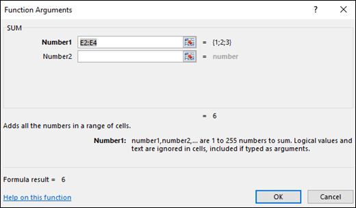
To make it easier to create and edit formulas and minimize typing and syntax errors, use Formula AutoComplete. After you type an = (equal sign) and beginning letters of a function, Excel displays a dynamic drop-down list of valid functions, arguments, and names that match those letters. You can then select one from the drop-down list and Excel will enter it for you.
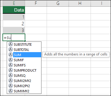
Nesting Excel functions
In certain cases, you may need to use a function as one of the arguments of another function. For example, the following formula uses a nested AVERAGE function and compares the result with the value 50.
1. The AVERAGE and SUM functions are nested within the IF function.
Valid returns When a nested function is used as an argument, the nested function must return the same type of value that the argument uses. For example, if the argument returns a TRUE or FALSE value, the nested function must return a TRUE or FALSE value. If the function doesn’t, Excel displays a #VALUE! error value.
Nesting level limits A formula can contain up to seven levels of nested functions. When one function (we’ll call this Function B) is used as an argument in another function (we’ll call this Function A), Function B acts as a second-level function. For example, the AVERAGE function and the SUM function are both second-level functions if they are used as arguments of the IF function. A function nested within the nested AVERAGE function is then a third-level function, and so on.
Источник
Using functions and nested functions in Excel formulas
Functions are predefined formulas that perform calculations by using specific values, called arguments, in a particular order, or structure. Functions can be used to perform simple or complex calculations. You can find all of Excel’s functions on the Formulas tab on the Ribbon:
Excel function syntax
The following example of the ROUND function rounding off a number in cell A10 illustrates a function’s syntax.
1. Structure. The structure of a function begins with an equal sign (=), followed by the function name, an opening parenthesis, the arguments for the function separated by commas, and a closing parenthesis.
2. Function name. For a list of available functions, click a cell and press SHIFT+F3, which will launch the Insert Function dialog.
3. Arguments. Arguments can be numbers, text, logical values such as TRUE or FALSE, arrays, error values such as #N/A, or cell references. The argument you designate must produce a valid value for that argument. Arguments can also be constants, formulas, or other functions.
4. Argument tooltip. A tooltip with the syntax and arguments appears as you type the function. For example, type =ROUND( and the tooltip appears. Tooltips appear only for built-in functions.
Note: You don’t need to type functions in all caps, like =ROUND, as Excel will automatically capitalize the function name for you once you press enter. If you misspell a function name, like =SUME(A1:A10) instead of =SUM(A1:A10), then Excel will return a #NAME? error.
Entering Excel functions
When you create a formula that contains a function, you can use the Insert Function dialog box to help you enter worksheet functions. Once you select a function from the Insert Function dialog Excel will launch a function wizard, which displays the name of the function, each of its arguments, a description of the function and each argument, the current result of the function, and the current result of the entire formula.
To make it easier to create and edit formulas and minimize typing and syntax errors, use Formula AutoComplete. After you type an = (equal sign) and beginning letters of a function, Excel displays a dynamic drop-down list of valid functions, arguments, and names that match those letters. You can then select one from the drop-down list and Excel will enter it for you.
Nesting Excel functions
In certain cases, you may need to use a function as one of the arguments of another function. For example, the following formula uses a nested AVERAGE function and compares the result with the value 50.
1. The AVERAGE and SUM functions are nested within the IF function.
Valid returns When a nested function is used as an argument, the nested function must return the same type of value that the argument uses. For example, if the argument returns a TRUE or FALSE value, the nested function must return a TRUE or FALSE value. If the function doesn’t, Excel displays a #VALUE! error value.
Nesting level limits A formula can contain up to seven levels of nested functions. When one function (we’ll call this Function B) is used as an argument in another function (we’ll call this Function A), Function B acts as a second-level function. For example, the AVERAGE function and the SUM function are both second-level functions if they are used as arguments of the IF function. A function nested within the nested AVERAGE function is then a third-level function, and so on.
Источник
101 Excel Functions you should know
Summary
Excel contains over 500 functions, with more functions added every year. That is a huge number, so where should you start? This guide provides a walkthrough of over 100 important functions in Excel with many examples and links. Click function names for details and more examples.
Below is a brief overview of about 100 important Excel functions you should know, with links to detailed examples. We also have a large list of example formulas, a more complete list of Excel functions, and video training. If you are new to Excel formulas, see this introduction.
Note: Excel now includes Dynamic Array formulas, which offer important new functions.
Date and Time Functions
Excel provides many functions to work with dates and times.
NOW and TODAY
You can get the current date with the TODAY function and the current date and time with the NOW Function. Technically, the NOW function returns the current date and time, but you can format as time only, as seen below:

Note: these are volatile functions and will recalculate with every worksheet change. If you want a static value, use date and time shortcuts.
DAY, MONTH, YEAR, and DATE
You can use the DAY, MONTH, and YEAR functions to disassemble any date into its raw components, and the DATE function to put things back together again.
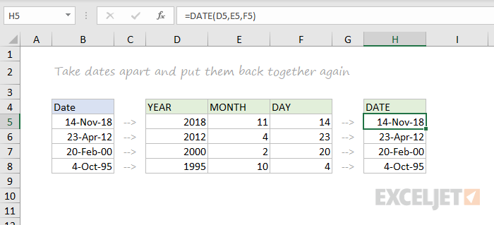
HOUR, MINUTE, SECOND, and TIME
Excel provides a set of parallel functions for times. You can use the HOUR, MINUTE, and SECOND functions to extract pieces of a time, and you can assemble a TIME from individual components with the TIME function.
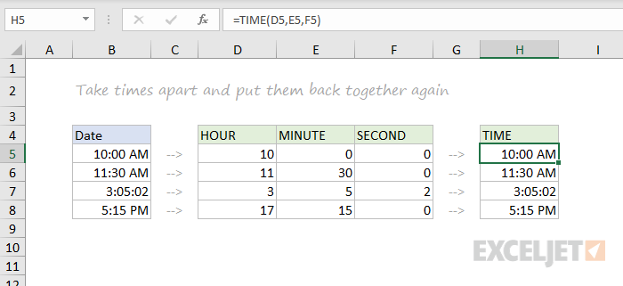
DATEDIF and YEARFRAC
You can use the DATEDIF function to get time between dates in years, months, or days. DATEDIF can also be configured to get total time in «normalized» denominations, i.e. «2 years and 6 months and 27 days».
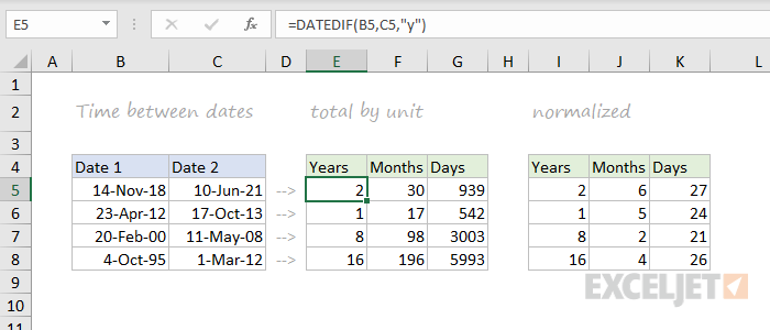
Use YEARFRAC to get fractional years:
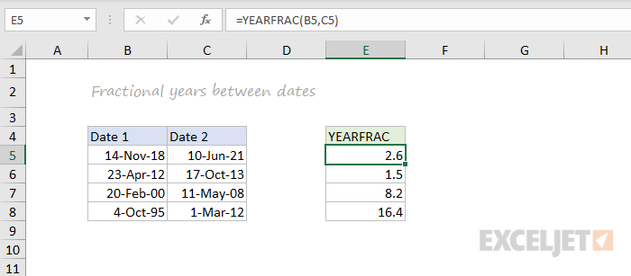
EDATE and EOMONTH
A common task with dates is to shift a date forward (or backward) by a given number of months. You can use the EDATE and EOMONTH functions for this. EDATE moves by month and retains the day. EOMONTH works the same way, but always returns the last day of the month.
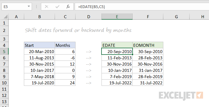
WORKDAY and NETWORKDAYS
To figure out a date n working days in the future, you can use the WORKDAY function. To calculate the number of workdays between two dates, you can use NETWORKDAYS.
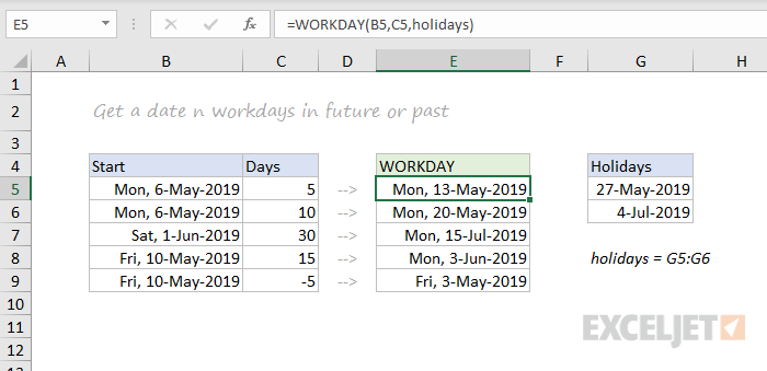
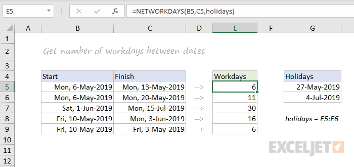
Note: Both functions automatically skip weekends (Saturday and Sunday) and will also skip holidays, if provided. If you need more flexibility on what days are considered weekends, see the WORKDAY.INTL function and NETWORKDAYS.INTL function.
WEEKDAY and WEEKNUM
To figure out the day of week from a date, Excel provides the WEEKDAY function. WEEKDAY returns a number between 1-7 that indicates Sunday, Monday, Tuesday, etc. Use the WEEKNUM function to get the week number in a given year.
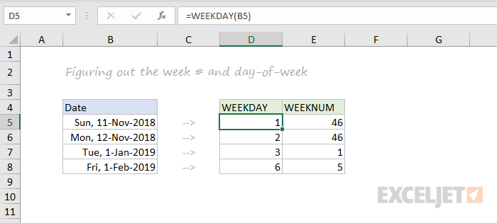
Engineering
CONVERT
Most Engineering functions are pretty technical. you’ll find a lot of functions for complex numbers in this section. However, the CONVERT function is quite useful for everyday unit conversions. You can use CONVERT to change units for distance, weight, temperature, and much more.
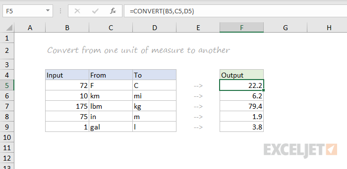
Information Functions
ISBLANK, ISERROR, ISNUMBER, and ISFORMULA
Excel provides many functions for checking the value in a cell, including ISNUMBER, ISTEXT, ISLOGICAL, ISBLANK, ISERROR, and ISFORMULA These functions are sometimes called the «IS» functions, and they all return TRUE or FALSE based on a cell’s contents.
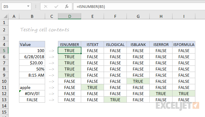
Excel also has ISODD and ISEVEN functions that will test a number to see if it’s even or odd.
By the way, the green fill in the screenshot above is applied automatically with a conditional formatting formula.
Logical Functions
Excel’s logical functions are a key building block of many advanced formulas. Logical functions return the boolean values TRUE or FALSE. If you need a primer on logical formulas, this video goes through many examples.
AND, OR and NOT
The core of Excel’s logical functions are the AND function, the OR function, and the NOT function. In the screen below, each of these function is used to run a simple test on the values in column B:
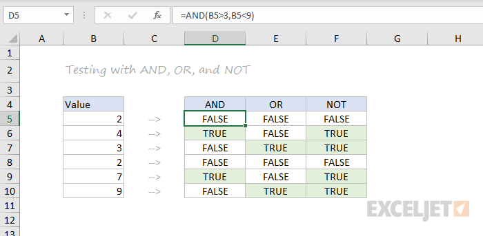
IFERROR and IFNA
The IFERROR function and IFNA function can be used as a simple way to trap and handle errors. In the screen below, VLOOKUP is used to retrieve cost from a menu item. Column F contains just a VLOOKUP function, with no error handling. Column G shows how to use IFNA with VLOOKUP to display a custom message when an unrecognized item is entered.
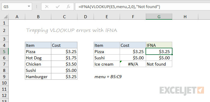
Whereas IFNA only catches an #N/A error, the IFERROR function will catch any formula error.
IF and IFS functions
The IF function is one of the most used functions in Excel. In the screen below, IF checks test scores and assigns «pass» or «fail»:
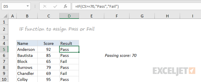
Multiple IF functions can be nested together to perform more complex logical tests.
New in Excel 2019 and Excel 365, the IFS function can run multiple logical tests without nesting IFs.
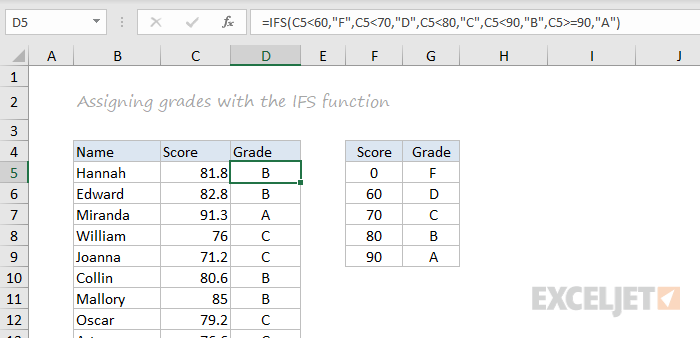
Lookup and Reference Functions
VLOOKUP and HLOOKUP
Excel offers a number of functions to lookup and retrieve data. Most famous of all is VLOOKUP:
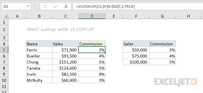
HLOOKUP works like VLOOKUP, but expects data arranged horizontally:
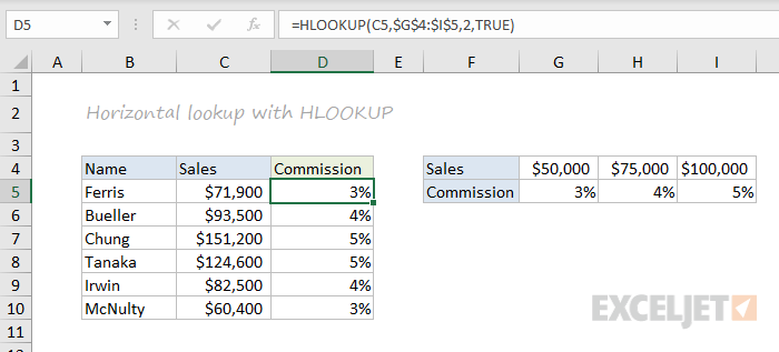
INDEX and MATCH
For more complicated lookups, INDEX and MATCH offers more flexibility and power:
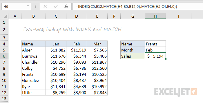
Both the INDEX function and the MATCH function are powerhouse functions that turn up in all kinds of formulas.
LOOKUP
The LOOKUP function has default behaviors that make it useful when solving certain problems. LOOKUP assumes values are sorted in ascending order and always performs an approximate match. When LOOKUP can’t find a match, it will match the next smallest value. In the example below we are using LOOKUP to find the last entry in a column:
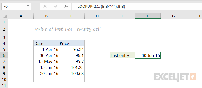
ROW and COLUMN
You can use the ROW function and COLUMN function to find row and column numbers on a worksheet. Notice both ROW and COLUMN return values for the current cell if no reference is supplied:
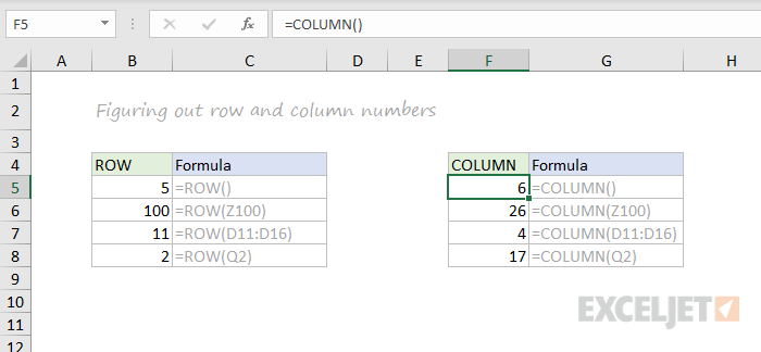
The row function also shows up often in advanced formulas that process data with relative row numbers.
ROWS and COLUMNS
The ROWS function and COLUMNS function provide a count of rows in a reference. In the screen below, we are counting rows and columns in an Excel Table named «Table1».
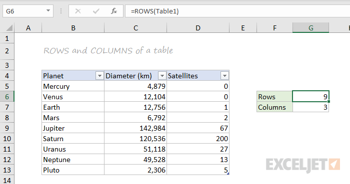
Note ROWS returns a count of data rows in a table, excluding the header row. By the way, here are 23 things to know about Excel Tables.
HYPERLINK
You can use the HYPERLINK function to construct a link with a formula. Note HYPERLINK lets you build both external links and internal links:
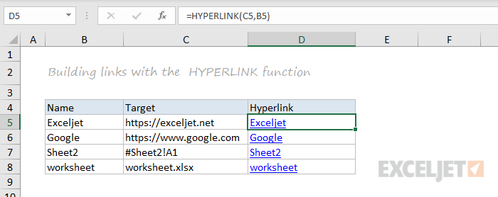
GETPIVOTDATA
The GETPIVOTDATA function is useful for retrieving information from existing pivot tables.
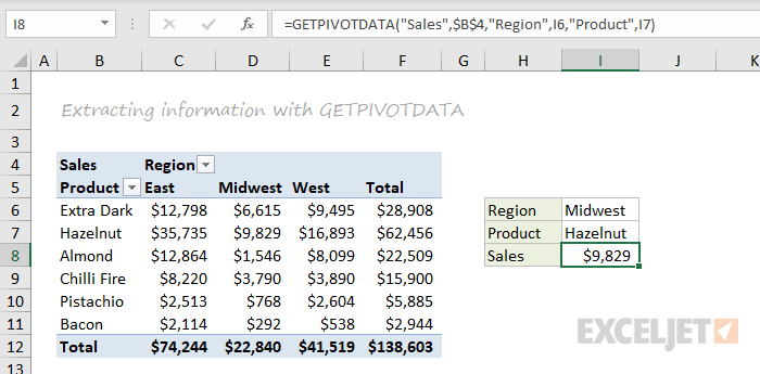
CHOOSE
The CHOOSE function is handy any time you need to make a choice based on a number:
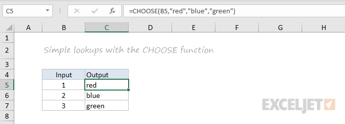
TRANSPOSE
The TRANSPOSE function gives you an easy way to transpose vertical data to horizontal, and vice versa.
![]()
Note: TRANSPOSE is a formula and is, therefore, dynamic. If you just need to do a one-time transpose operation, use Paste Special instead.
OFFSET
The OFFSET function is useful for all kinds of dynamic ranges. From a starting location, it lets you specify row and column offsets, and also the final row and column size. The result is a range that can respond dynamically to changing conditions and inputs. You can feed this range to other functions, as in the screen below, where OFFSET builds a range that is fed to the SUM function:
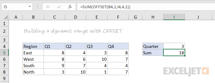
INDIRECT
The INDIRECT function allows you to build references as text. This concept is a bit tricky to understand at first, but it can be useful in many situations. Below, we are using INDIRECT to get values from cell A1 in 5 different worksheets. Each reference is dynamic. If a sheet name changes, the reference will update.
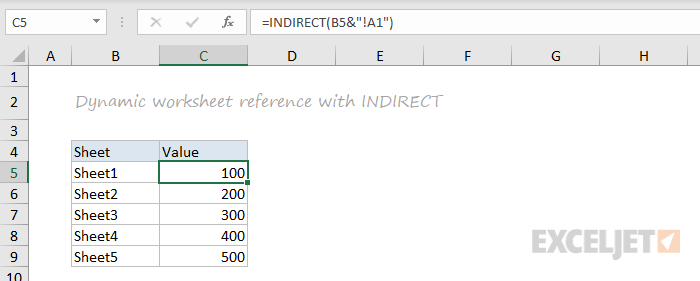
The INDIRECT function is also used to «lock» references so they won’t change, when rows or columns are added or deleted. For more details, see linked examples at the bottom of the INDIRECT function page.
Caution: both OFFSET and INDIRECT are volatile functions and can slow down large or complicated spreadsheets.
STATISTICAL Functions
COUNT and COUNTA
You can count numbers with the COUNT function and non-empty cells with COUNTA. You can count blank cells with COUNTBLANK, but in the screen below we are counting blank cells with COUNTIF, which is more generally useful.
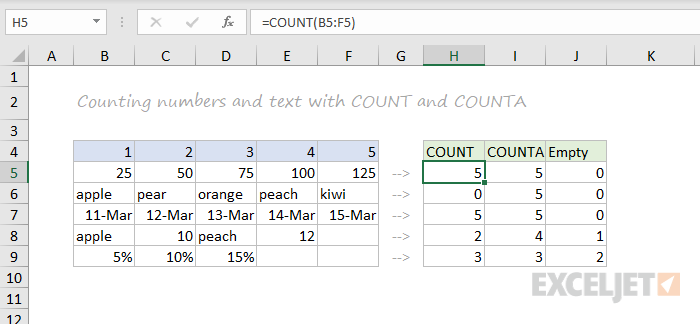
COUNTIF and COUNTIFS
For conditional counts, the COUNTIF function can apply one criteria. The COUNTIFS function can apply multiple criteria at the same time:
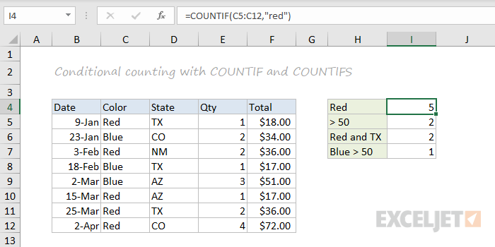
SUM, SUMIF, SUMIFS
To sum everything, use the SUM function. To sum conditionally, use SUMIF or SUMIFS. Following the same pattern as the counting functions, the SUMIF function can apply only one criteria while the SUMIFS function can apply multiple criteria.
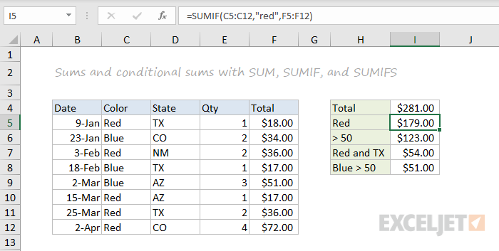
AVERAGE, AVERAGEIF, and AVERAGEIFS
Following the same pattern, you can calculate an average with AVERAGE, AVERAGEIF, and AVERAGEIFS.
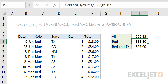
MIN, MAX, LARGE, SMALL
You can find largest and smallest values with MAX and MIN, and nth largest and smallest values with LARGE and SMALL. In the screen below, data is the named range C5:C13, used in all formulas.
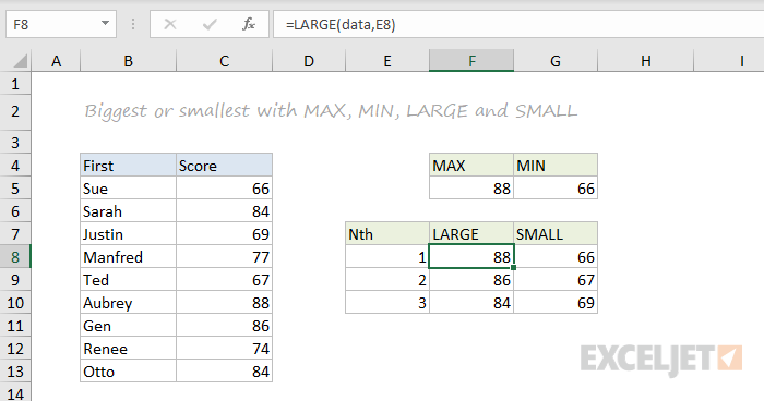
MINIFS, MAXIFS
The MINIFS and MAXIFS. These functions let you find minimum and maximum values with conditions:
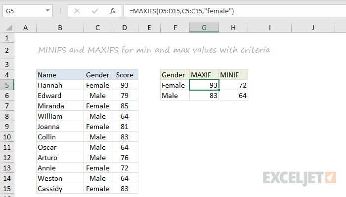
Note: MINIFS and MAXIFS are new in Excel via Office 365 and Excel 2019.
The MODE function returns the most commonly occurring number in a range:
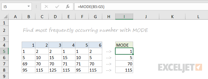
To rank values largest to smallest, or smallest to largest, use the RANK function:
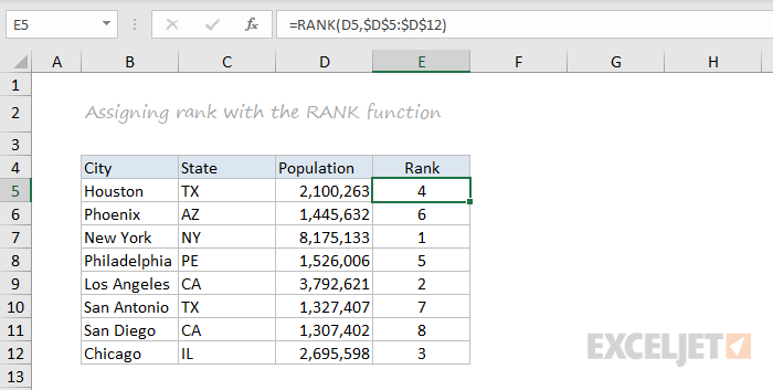
MATH Functions
To change negative values to positive use the ABS function.
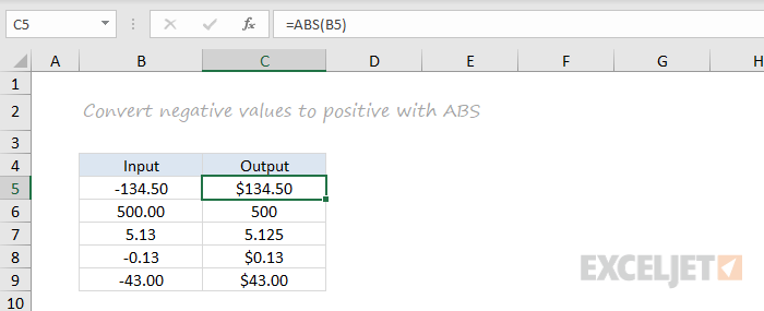
RAND and RANDBETWEEN
Both the RAND function and RANDBETWEEN function can generate random numbers on the fly. RAND creates long decimal numbers between zero and 1. RANDBETWEEN generates random integers between two given numbers.
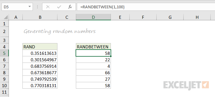
ROUND, ROUNDUP, ROUNDDOWN, INT
To round values up or down, use the ROUND function. To force rounding up to a given number of digits, use ROUNDUP. To force rounding down, use ROUNDDOWN. To discard the decimal part of a number altogether, use the INT function.
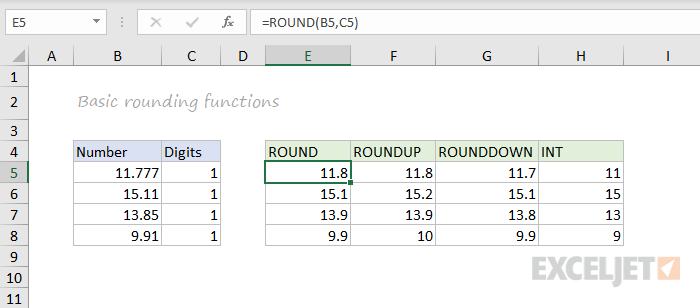
MROUND, CEILING, FLOOR
To round values to the nearest multiple use the MROUND function. The FLOOR function and CEILING function also round to a given multiple. FLOOR forces rounding down, and CEILING forces rounding up.
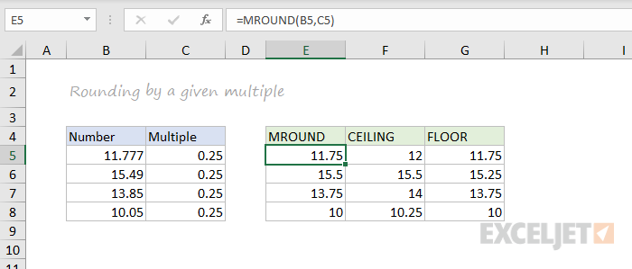
The MOD function returns the remainder after division. This sounds boring and geeky, but MOD turns up in all kinds of formulas, especially formulas that need to do something «every nth time». In the screen below, you can see how MOD returns zero every third number when the divisor is 3:
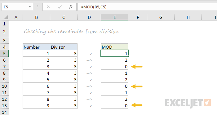
SUMPRODUCT
The SUMPRODUCT function is a powerful and versatile tool when dealing with all kinds of data. You can use SUMPRODUCT to easily count and sum based on criteria, and you can use it in elegant ways that just don’t work with COUNTIFS and SUMIFS. In the screen below, we are using SUMPRODUCT to count and sum orders in March. See the SUMPRODUCT page for details and links to many examples.
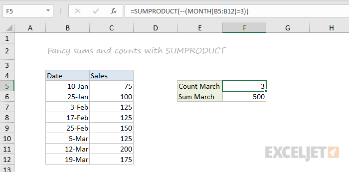
SUBTOTAL
The SUBTOTAL function is an «aggregate function» that can perform a number of operations on a set of data. All told, SUBTOTAL can perform 11 operations, including SUM, AVERAGE, COUNT, MAX, MIN, etc. (see this page for the full list). The key feature of SUBTOTAL is that it will ignore rows that have been «filtered out» of an Excel Table, and, optionally, rows that have been manually hidden. In the screen below, SUBTOTAL is used to count and sum only the 7 visible rows in the table:
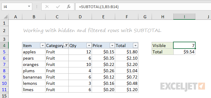
AGGREGATE
Like SUBTOTAL, the AGGREGATE function can also run a number of aggregate operations on a set of data and can optionally ignore hidden rows. The key differences are that AGGREGATE can run more operations (19 total) and can also ignore errors.
In the screen below, AGGREGATE is used to perform MIN, MAX, LARGE and SMALL operations while ignoring errors. Normally, the error in cell B9 would prevent these functions from returning a result. See this page for a full list of operations AGGREGATE can perform.
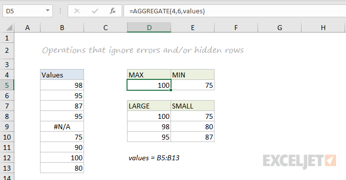
TEXT Functions
LEFT, RIGHT, MID
To extract characters from the left, right, or middle of text, use LEFT, RIGHT, and MID functions:
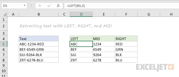
The LEN function will return the length of a text string. LEN shows up in a lot of formulas that count words or characters.
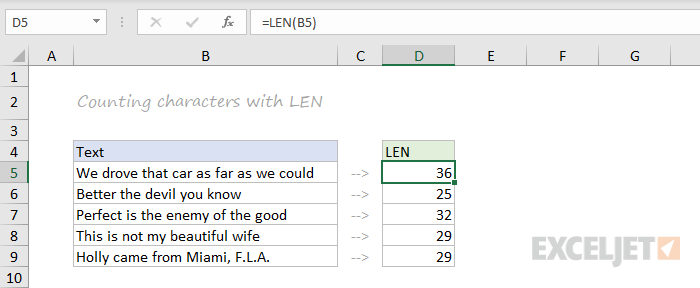
FIND, SEARCH
To look for specific text in a cell, use the FIND function or SEARCH function. These functions return the numeric position of matching text, but SEARCH allows wildcards and FIND is case-sensitive. Both functions will throw an error when text is not found, so wrap in the ISNUMBER function to return TRUE or FALSE (example here).
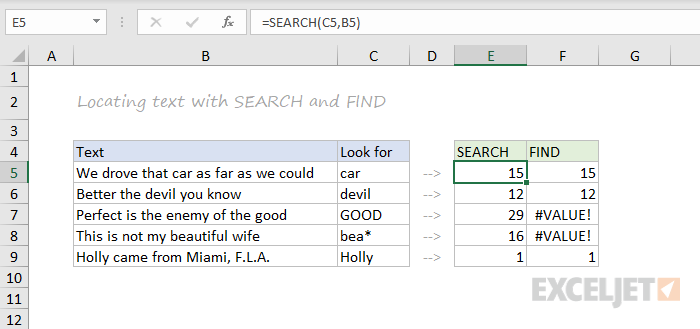
REPLACE, SUBSTITUTE
To replace text by position, use the REPLACE function. To replace text by matching, use the SUBSTITUTE function. In the first example, REPLACE removes the two asterisks (**) by replacing the first two characters with an empty string («»). In the second example, SUBSTITUTE removes all hash characters (#) by replacing «#» with «».
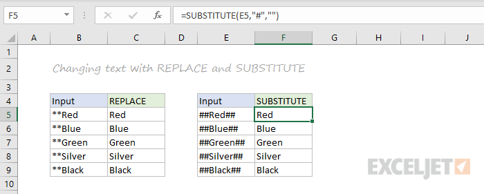
CODE, CHAR
To figure out the numeric code for a character, use the CODE function. To translate the numeric code back to a character, use the CHAR function. In the example below, CODE translates each character in column B to its corresponding code. In column F, CHAR translates the code back to a character.
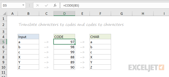
TRIM, CLEAN
To get rid of extra space in text, use the TRIM function. To remove line breaks and other non-printing characters, use CLEAN.
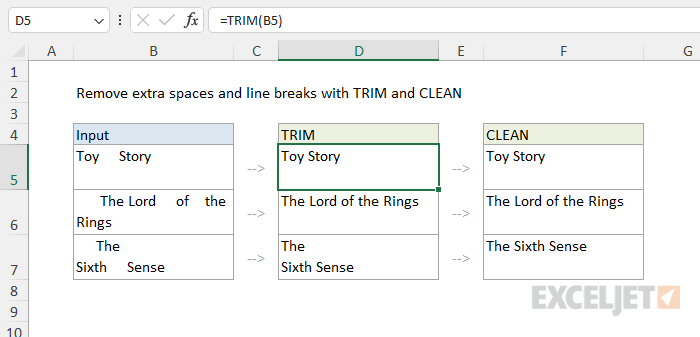
CONCAT, TEXTJOIN, CONCATENATE
New in Excel via Office 365 are CONCAT and TEXTJOIN. The CONCAT function lets you concatenate (join) multiple values, including a range of values without a delimiter. The TEXTJOIN function does the same thing, but allows you to specify a delimiter and can also ignore empty values.
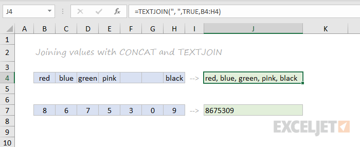
Excel also provides the CONCATENATE function, but it doesn’t offer special features. I wouldn’t bother with it and would instead concatenate directly with the ampersand (&) character in a formula.
EXACT
The EXACT function allows you to compare two text strings in a case-sensitive manner.
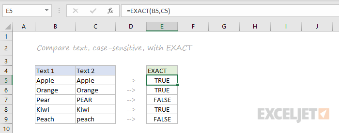
UPPER, LOWER, PROPER
To change the case of text, use the UPPER, LOWER, and PROPER function
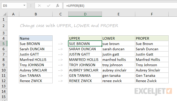
Last but definitely not least is the TEXT function. The text function lets you apply number formatting to numbers (including dates, times, etc.) as text. This is especially useful when you need to embed a formatted number in a message, like «Sale ends on [date]».
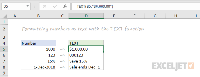
Dynamic Array functions
Dynamic arrays are new in Excel 365, and are a major upgrade to Excel’s formula engine. As part of the dynamic array update, Excel includes new functions which directly leverage dynamic arrays to solve problems that are traditionally hard to solve with conventional formulas. If you are using Excel 365, make sure you are aware of these new functions:
Источник