
Follow these steps to fill a formula and choose which options to apply:
-
Select the cell that has the formula you want to fill into adjacent cells.
-
Drag the fill handle
 across the cells that you want to fill.
If you don’t see the fill handle, it might be hidden. To display it again:
-
Click File > Options
-
Click Advanced.
-
Under Editing Options, check the Enable fill handle and cell drag-and-drop box.
-
-
To change how you want to fill the selection, click the small Auto Fill Options icon
that appears after you finish dragging, and choose the option that want.
 across the cells that you want to fill.
 that appears after you finish dragging, and choose the option that want.
For more information about copying formulas, see Copy and paste a formula to another cell or worksheet.
Fill formulas into adjacent cells
You can use the Fill command to fill a formula into an adjacent range of cells. Simply do the following:
-
Select the cell with the formula and the adjacent cells you want to fill.
-
Click Home > Fill, and choose either Down, Right, Up, or Left.
Keyboard shortcut: You can also press Ctrl+D to fill the formula down in a column, or Ctrl+R to fill the formula to the right in a row.
Turn workbook calculation on
Formulas won’t recalculate when you fill cells if automatic workbook calculation isn’t enabled.
Here’s how you can enable it:
-
Click File > Options.
-
Click Formulas.
-
Under Workbook Calculation, choose Automatic.
-
Select the cell that has the formula you want to fill into adjacent cells.
-
Drag the fill handle
down or to the right of the column you want to fill.
 down or to the right of the column you want to fill.
Keyboard shortcut: You can also press Ctrl+D to fill the formula down a cell in a column, or Ctrl+R to fill the formula to the right in a row.
Copying and Pasting a cell or a range of cells is one of the most common tasks users do in Excel.
A proper understanding of how to copy-paste multiple cells (that are adjacent or non-adjacent) would really help you be a lot more efficient while working with Microsoft Excel.
In this tutorial, I will show you different scenarios where you can copy and paste multiple cells in Excel.
If you have been using Excel for some time now, I’m quite sure you would know some of these already, but there’s a good chance you’d end up learning something new.
So let’s get started!
Copy and Paste Multiple Adjacent Cells
Let’s start with the easy scenario.
Suppose you have a range of cells (that are adjacent) as shown below and you want to copy it to some other location in the same worksheet or some other worksheet/workbook.

Below are the steps to do this:
- Select the range of cells that you want to copy

- Right-click on the selection
- Click on Copy

- Right-click on the destination cell (E1 in this example)
- Click on the Paste icon
The above steps would copy all the cells in the selected range and paste them into the destination range.

In case you already have something in the destination range, it would be overwritten.
Excel also gives you the flexibility to choose what you want to paste. For example, you can choose to only copy and paste the values, or the formatting, or the formulas, etc.
These options are available to you when you right-click on the destination cell (the icons below the paste special option).
Or you can click on the Paste Special option and then choose what you want to paste using the options in the dialog box.
Useful Keyboard Shortcuts for Copy Paste
In case you prefer using the keyboard while working with Excel, you can use the below shortcut:
- Control + C (Windows) or Command + C (Mac) – to copy range of cells
- Control + V (Windows) or Command + V (Mac) – to paste in the destination cells
And below are some advanced copy-paste shortcuts (using the paste special dialog box).
To use this, first copy the cells, then select the destination cell, and then use the below keyboard shortcuts.
- To paste only the Values – Control + E + S + V + Enter
- To paste only the Formulas – Control + E + S + F + Enter
- To paste only the Formatting – Control + E + S + T + Enter
- To paste only the Column Width – Control + E + S + W + Enter
- To paste only the Comments and notes – Control + E + S + C + Enter
In case you’re using Mac, use Command instead of Control.
Also read: How to Cut a Cell Value in Excel (Keyboard Shortcuts)
Mouse Shortcut for Copy Paste
If you prefer using the mouse instead of the keyboard shortcuts, here is another way you can quickly copy and paste multiple cells in Excel.
- Select the cells that you want to copy
- Hold the Control key
- Place the mouse cursor at the edge of the selection (you will notice that the cursor changes into an arrow with a plus sign)
- Left-click and then drag the selection where you want the cells to be pasted

This method is also quite fast but is only useful in case you want to copy and paste the range of cells in the same worksheet somewhere nearby.
If the destination cell is a little far off, you’re better off using the keyboard shortcuts.
Copy and Paste Multiple Non-Adjacent Cells
Copy-pasting multiple cells that are nonadjacent is a bit tricky.
If you select multiple cells that are not adjacent to each other, and you copy these cells, you’ll see a prompt as shown below.

This is Excel’s way of telling you that you cannot copy multiple cells that are non-adjacent.
Unfortunately, there’s nothing that you can do about it.
There’s no hack or a workaround, and if you want to copy and paste these nonadjacent cells, you will have to do this one by one.
But there are a few scenarios where you can actually copy and paste non-adjacent cells in Excel.
Let’s have a look at these.
Copy and Paste Multiple Non-Adjacent Cells (that are in the same row/column)
While you can not copy non-adjacent cells in different rows and columns, if you have non-adjacent cells in the same row or column, Excel allows you to copy these.
For example, you can copy cells in the same row (even if these are non-adjacent). Just select the cells and then use Control + C (or Command + C for Mac). You will see the outline (the dancing ants outline).

Once you have copied these cells, go to the destination cell and paste these (Control + V or Command + V)
Excel will paste all the copied cells in the destination cell but make these adjacents.
Similarly, you can select multiple nonadjacent cells in one column, copy them, and then paste it into the destination cells.
Copy and Paste Multiple Non-Adjacent Rows/Columns (but adjacent cells)
Another thing Excel allows is to select non-adjacent rows or non-adjacent columns and then copy them.

Now when you paste these in the destination cell, these would be pasted as adjacent rows or columns.

Below is an example where I copied multiple non-adjacent rows from the dataset and pasted these in a different location.
Copy Value From Above in Non-Adjacent Cells
One practical scenario where you may have to copy and paste multiple cells would be when you have gaps in a data set and you want to copy the value from the cell above.
Below I have some dates in column A, and there are some blank cells as well. I want to fill these blank cells with the date in the last filed cell above them.

To do this, I would need to do two things:
- Select all the blank cells
- Copy the date from the above-filled cell and paste it into these blank cells
Let me show you how to do this.
Select All Blank Cells in the Dataset
Below are the steps to select all the blank cells in column A:
- Select the dates in column A, including the blank ones that you want to fill

- Press the F5 key on your keyboard. This will open the Go To dialog box.
- Click the Special button. This will open the Go To Special dialog box.

- In the Go To Special dialog box, select Blanks

- Click OK
The above steps would select all the blank cells in column A.

Now, we want to somehow copy the value in the above field cell in these blank cells. This cannot be done using any copy-paste method so we will have to use a formula (a very simple one).
Fill Blank Cells with Value Above
This part is really easy.
- With the blank cell selected, first hit the equal to key on your keyboard

- Now hit the Up arrow key. This will automatically enter the cell reference of the cell that is above the active cell.

- Hold the Control key and press the Enter key
The above steps would enter the same formula in all the selected blank cells – which is to refer to the cell above it.

While this is a formula, the end result is that you have the blank cells filled with the above-filled date in the data set.
Once you have the desired result, you can convert the formula into values if you want (so that the formula doesn’t update the cells in case you change any value in a cell that is being referenced in the formula).
So these are a couple of methods you can use to copy and paste multiple cells (adjacent and non-adjacent cells) in Excel. I am sure using these methods will help you save tons of time in your day-to-day work.
I hope you found this tutorial useful!
Other Excel tutorials you may also like:
- How to Copy and Paste Column in Excel? 3 Easy Ways!
- How to Copy Excel Table to MS Word (4 Easy Ways)
- How to Copy Conditional Formatting to Another Cell in Excel
- How to Copy and Paste Formulas in Excel without Changing Cell References
- How to Edit Cells in Excel?
To select a range, select a cell, then with the left mouse button pressed, drag over the other cells. Or use the Shift + arrow keys to select the range. To select non-adjacent cells and cell ranges, hold Ctrl and select the cells.
Contents
- 1 How do you select multiple cells individually?
- 2 How do you select two columns in Excel that are not next to each other on Mac?
- 3 How do you select multiple cells in Excel without dragging?
- 4 How do I select only certain cells in Excel?
- 5 Why can’t I select multiple cells in Excel?
- 6 How do I select two columns in another worksheet?
- 7 How do I highlight two non adjacent cells in Excel?
- 8 How do I copy multiple non adjacent cells in Excel?
- 9 How do you delete multiple columns in Excel not next to each other?
- 10 When should you use Ctrl key method for selecting multiple cells?
- 11 How do I select a large range of cells in Excel without scrolling?
- 12 What is an Xlookup in Excel?
- 13 How do I select multiple cells in Excel to copy and paste?
- 14 How do you group multiple selections in Excel?
- 15 How do I select multiple cells in sheets?
- 16 How do I select certain cells in sheets?
- 17 How do I paste into multiple cells in sheets?
- 18 How do you select two non-adjacent columns in sheets?
- 19 How do you copy multiple cells into one cell?
- 20 How do you copy consecutive cells in Excel?
How do you select multiple cells individually?
Hold the Control key on the keyboard. One by one, select all the non-contiguous cells (or range of cells) that you want to remain selected. When done, leave the Control key.
How do you select two columns in Excel that are not next to each other on Mac?
Select multiple adjacent rows or columns: Click the number or letter for the first row or column, then drag a white dot across the adjacent rows or columns. Select nonadjacent rows or columns: Command-click any row numbers or column letters.
How do you select multiple cells in Excel without dragging?
Select a Large Range of Cells With the Shift Key
Click the first cell in the range you want to select. Scroll your sheet until you find the last cell in the range you want to select. Hold down your Shift key, and then click that cell. All the cells in the range are now selected.
How do I select only certain cells in Excel?
Select one or more cells
- Click on a cell to select it. Or use the keyboard to navigate to it and select it.
- To select a range, select a cell, then with the left mouse button pressed, drag over the other cells.
- To select non-adjacent cells and cell ranges, hold Ctrl and select the cells.
Why can’t I select multiple cells in Excel?
Extend Selection Mode
If you notice some weird selection behavior going on with your mouse in Excel, take a look at the Status Bar — you might see something toward the left end that says “Extend Selection.” Even if you don’t, turning the selection mode off is easy. Just press F8.
How do I select two columns in another worksheet?
To select multiple columns or rows that are contiguous:
- Click on the first column or row in the group.
- Hold down the Shift key.
- Click the last column or row in the group.
How do I highlight two non adjacent cells in Excel?
Select Non-Adjacent Cells with Keyboard and Mouse
- With your mouse, click the first cell you want to highlight.
- Press and hold the Ctrl key on the keyboard.
- Click the rest of the cells you want to highlight.
- Once the desired cells are highlighted, release the Ctrl key.
How do I copy multiple non adjacent cells in Excel?
(2) Copy and paste multiple non adjacent rows (or columns) which contain the same columns (or rows) 1. Holding the Ctrl key, and select multiple nonadjacent rows (or columns) which contain the same columns (or rows).
How do you delete multiple columns in Excel not next to each other?
Hold down the Command key, and select each of the other rows of the group. After all rows are selected, right-click or control-click, and click Delete from the popup menu. Or, after all rows are selected, choose Edit from the main menu, and click Delete.
When should you use Ctrl key method for selecting multiple cells?
When should you use the Ctrl key method for selecting multiple cells? When the cells are scattered and spread around the spreadsheet.
How do I select a large range of cells in Excel without scrolling?
You can do this two ways:
- Click into the cell in the upper left corner of the range.
- Click into the Name Box and type the cell in the lower right corner of the range.
- Press SHIFT + Enter.
- Excel will select the entire range.
What is an Xlookup in Excel?
Use the XLOOKUP function to find things in a table or range by row.With XLOOKUP, you can look in one column for a search term, and return a result from the same row in another column, regardless of which side the return column is on.
How do I select multiple cells in Excel to copy and paste?
After selecting the range of cells press Ctrl + C together to copy the range of cells. Again, select a range of cells where you want to paste it and press on to Ctrl + V together to paste it. This is the easiest way of copying and pasting multiple cells altogether.
How do you group multiple selections in Excel?
To group rows or columns:
- Select the rows or columns you want to group. In this example, we’ll select columns A, B, and C.
- Select the Data tab on the Ribbon, then click the Group command. Clicking the Group command.
- The selected rows or columns will be grouped. In our example, columns A, B, and C are grouped together.
How do I select multiple cells in sheets?
To select more than one row in the data view, click one row, then hold the Control (Windows) or Command (Mac) key and select each of the other rows you wish to edit or remove. To select a continuous list, click one row, then hold the Shift key and click the last row.
How do I select certain cells in sheets?
To select non-adjacent cells, simply hold down the command key (for Mac users, PC users hold down the CTRL key) while making your selections.
How do I paste into multiple cells in sheets?
To include multiple cells, click on one, and without releasing the click, drag your mouse around adjacent cells to highlight them before copying. To paste to a cell, single-click on the cell where you’d like to paste in the information and press Ctrl + V (or right-click on the destination cell and select Paste).
How do you select two non-adjacent columns in sheets?
Holding down the CTRL key on the keyboard and dragging over the required cells with the mouse is the only way that non-adjacent columns and cells can be selected in Google Sheets.
How do you copy multiple cells into one cell?
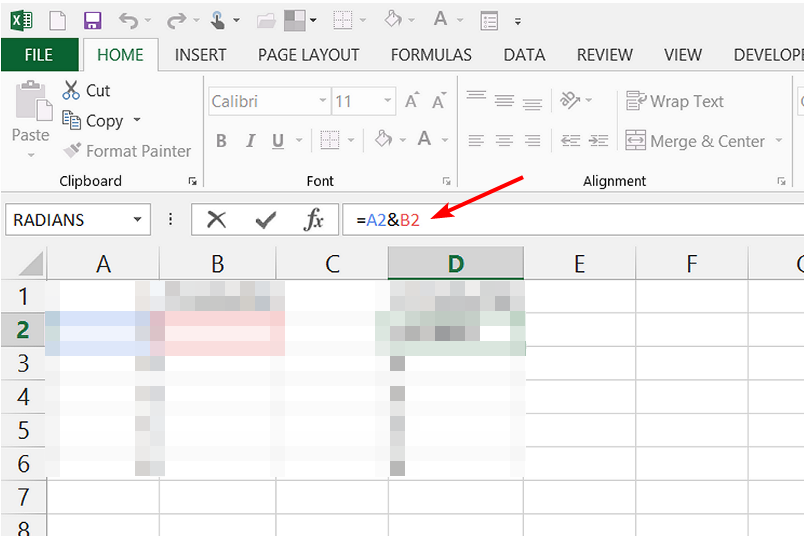
Combine text from two or more cells into one cell
- Select the cell where you want to put the combined data.
- Type = and select the first cell you want to combine.
- Type & and use quotation marks with a space enclosed.
- Select the next cell you want to combine and press enter. An example formula might be =A2&” “&B2.
How do you copy consecutive cells in Excel?
Simply select the cell containing the formula you want to fill into adjacent cells and drag the fill handle down the cells in the column or across the cells in the row that you want to fill. The formula is copied to the other cells.
This post will guide you how to merge adjacent cells in columns with same value or data with VBA Macro in Excel. How do I merge cells when adjacent value is the same in one column in Excel.
Assuming that you have a list of data in range A1:B4, and you only want to merge adjacent cells in column A. How to do it. You can use an Excel VBA Macro to quickly merge adjacent cells with same data or value in a specific column or range. Just do the following steps:
#1 open your excel workbook and then click on “Visual Basic” command under DEVELOPER Tab, or just press “ALT+F11” shortcut.

#2 then the “Visual Basic Editor” window will appear.
#3 click “Insert” ->”Module” to create a new module.

#4 paste the below VBA code into the code window. Then clicking “Save” button.
 Sub MergeAdjacentCells()

    Application.ScreenUpdating = False
    Application.DisplayAlerts = False

    Set myRange = Application.Selection
    Set myRange = Application.InputBox("Select one Range that you want to merge cells with same data in one column:", "MergeAdjacentCells", myRange.Address, Type:=8)

    MergeAgain:
    For Each myCell In myRange
       If myCell.Value = myCell.Offset(1, 0).Value And IsEmpty(myCell) = False Then
           Range(myCell, myCell.Offset(1, 0)).Merge
           GoTo MergeAgain
       End If
    Next
    Application.DisplayAlerts = True
    Application.ScreenUpdating = True
End Sub
#5 back to the current worksheet, then run the above excel macro. Click Run button.
#6 Select one Range that you want to merge cells with same data in one column. Click Ok button.
#7 let’s see the result:
Содержание
- How to Get Rid of the Green Triangle in Excel
- Switch Off Background Error Checking
- Error Checking Rules
- Ignore Error
- Use the Trace Error Drop Down
- Common Errors in Excel
- Cell Reference Error
- Value Error
- Adjacent Cells Error
- Excel Formula Omits Adjacent Cells Error
- How to get rid of this error?
- Getting rid of this error permanently
- Formula Omits Adjacent Cells Error in Excel: How to Fix It
- Ignore the Excel error or update your formula to include the cells
- What does the error formula omits adjacent cells mean in excel?
- What can I do if the Excel error formula omits adjacent cells?
- 1. Uncheck formulas that omit cells
- 2. Switch from absolute to relative reference
- 3. Update the formula to include the cells
- Adjacent cells omitted warning, why?
- Adjacent cells omitted warning, why?
- Re: Adjacent cells omitted warning, why?
- Re: Adjacent cells omitted warning, why?
- Re: Adjacent cells omitted warning, why?
- Re: Adjacent cells omitted warning, why?
- Re: [SOLVED] Adjacent cells omitted warning, why?
- Re: Adjacent cells omitted warning, why?
- Re: [SOLVED] Adjacent cells omitted warning, why?
- Re: [SOLVED] Adjacent cells omitted warning, why?
How to Get Rid of the Green Triangle in Excel
This tutorial demonstrates how to get rid of the green (trace error) triangle in Excel.
If the data contained in a cell has an error as defined by Excel, and background error checking is switched on, then a small green triangle is displayed in the top-left corner of a cell. If you click in the cell, you get a list of suggested fixes. On some occasions, you may not want to change the data in your cell, but just to hide the green triangle and ignore the error.
Switch Off Background Error Checking
To stop the green triangle error from showing, you can switch off background error checking in Excel.
- In the Ribbon, go to File > Options > Formulas > Error Checking.
- Remove the tick from the Enable background error checking option, and then click OK.
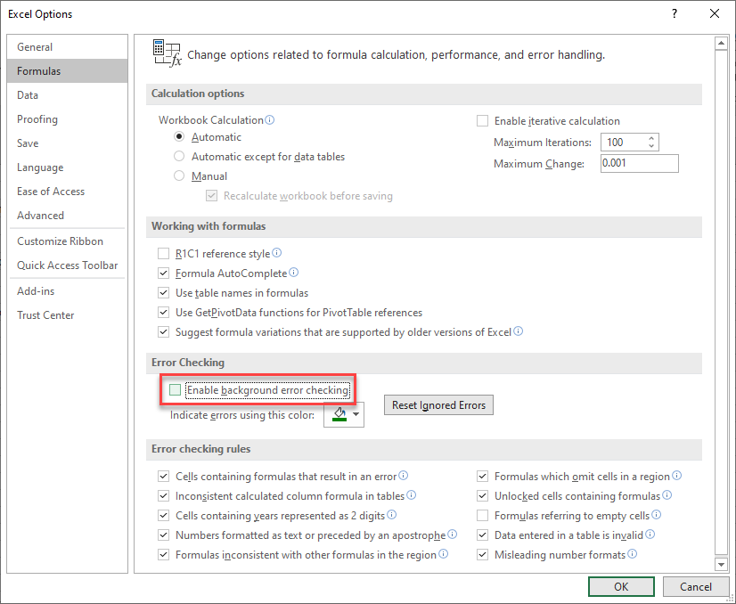
Note: This removes background error checking for the active workbook and any workbooks opened in the future.
Error Checking Rules
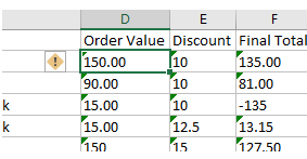
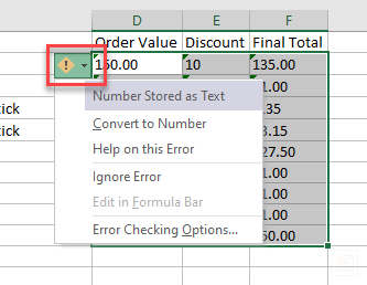
Instead of turning background error checking completely off, you can switch off individual rules that are switched on by default in Excel. For example, in the data above, the numbers are formatted as text and therefore cannot be used in calculation formulas. The green triangle alerts to this and provides a list of possible solutions. You can switch off this specific error check.
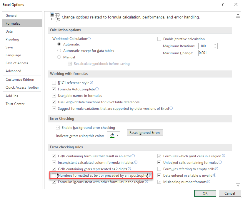
- In the Ribbon, select File > Options > Formulas > Error Checking.
- In the Error checking rules section, remove the check mark from Numbers formatted as text or preceded by an apostrophe to stop Excel from checking for this specific error, and then click OK.
Ignore Error
It’s generally best to keep the background error checking switched on, as it is very useful in showing you if you have an error in the data or in a formula.
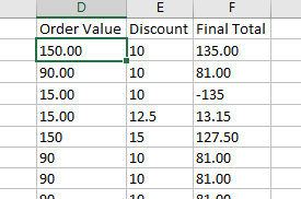
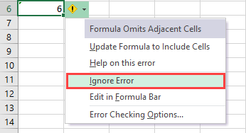
- To remove the green triangles from cells where you are aware of the error – but do not want to see the triangle – select the cells, and then click on the little yellow exclamation mark icon.
- Click Ignore Error to remove the green triangles, or if you want to solve the error, click Convert to Number, making the cell values suitable for use in calculations.
Use the Trace Error Drop Down
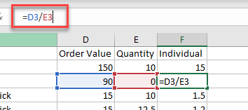
If your error has a different reason, for example a divide by zero formula error, then a different set of options is shown.
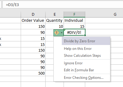
You can also ignore the error, or you can click Show Calculation Steps to resolve the error. If you click Edit in Formula Bar, Excel puts the formula into editing mode and place your mouse pointer in the formula bar so you can make changes to the formula.
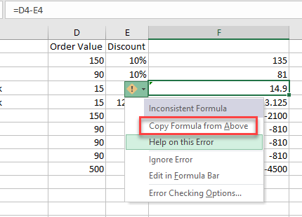
Another reason for the error could be an inconsistent formula. This occurs when the formula in the cell is different to the formula that is in the cell above. If this is the case, a different set of options appears.
To solve this problem and remove the green triangle, you can click Copy Formula from Above or, if you do not want to change the formula, you can, once again, click Ignore Error.
Common Errors in Excel
A few more common Excel errors can cause the green triangle to show in a cell – all of which can be removed using the Ignore Error option, or can be solved using Excel’s error checking options.
Cell Reference Error
#REF – this error normally occurs when a formula is referring to a range that is cannot find – or if rows/columns have been removed.
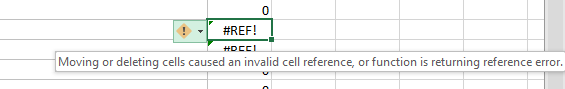
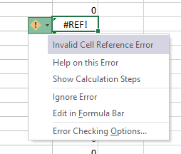
Resting your mouse on the exclamation mark icon shows you the reason for error, while clicking on the drop down shows you a list of possible solutions.
Value Error
#VALUE – this error normally occurs when you are trying to include a cell that has text in it, in a calculation.
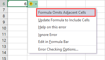
Adjacent Cells Error
Formula Omits Adjacent Cells – this error normally occurs when you have a function like the SUM Function and are not including all the possible cells in the calculation.
Источник
Excel Formula Omits Adjacent Cells Error
The Excel formula omits adjacent cell errors that can occur with mathematical or statistical functions, such as SUM, AVERAGE, COUNT, MIN, and MAX.
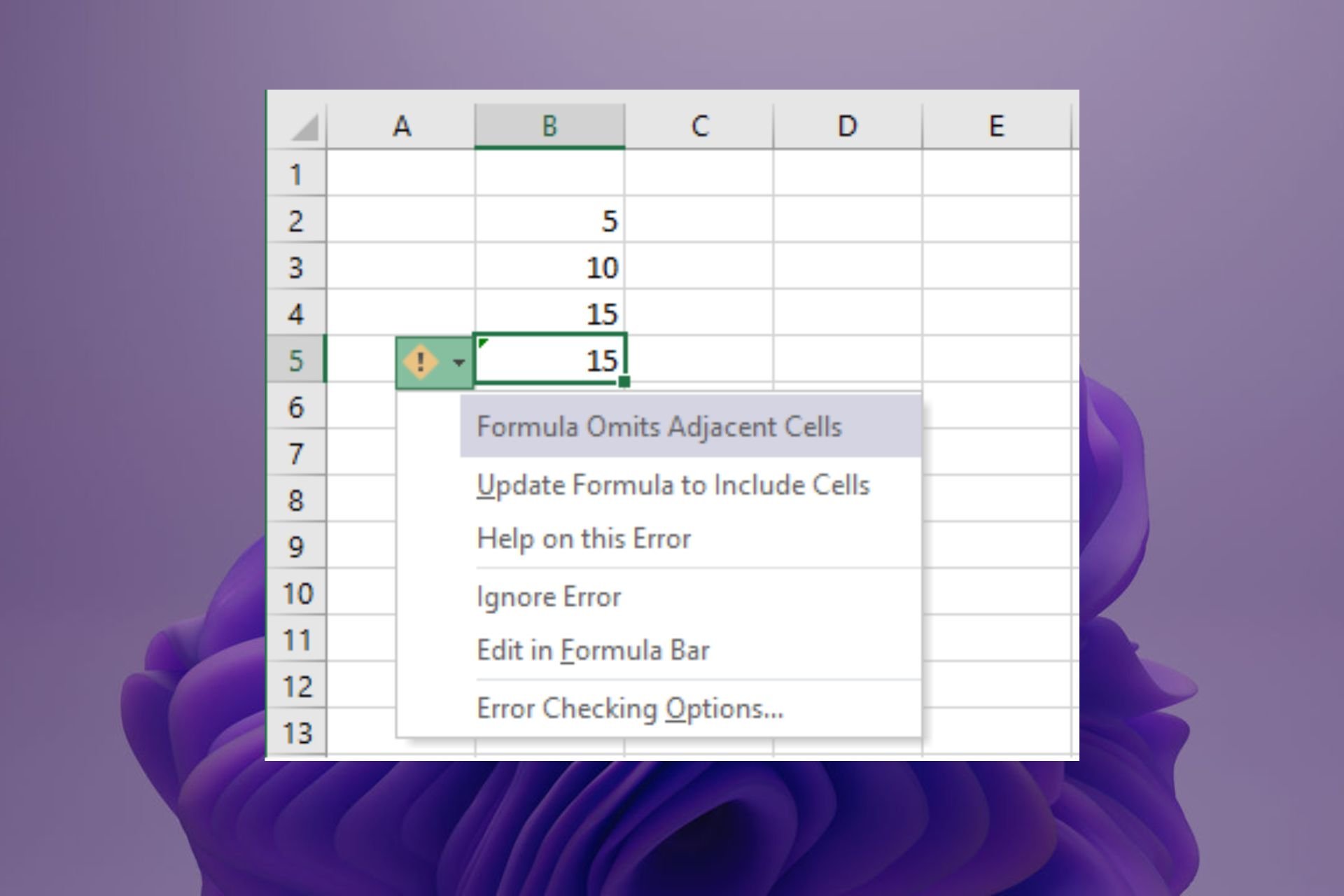
This error appears when there are cells with similar values to the one you chose that are not selected. Excel recognizes it as an error and symbolizes it with a little triangle.
I will illustrate it using the following example.
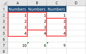
In cells A7, B7, and C7 you have the SUM function, summing cells in each column. Notice, that in the B and C columns, not all similar values are selected. In the A column, you also don’t have all cells selected (A1). But this is not the number type, so Excel understands it.
How to get rid of this error?
There are a few ways to make this error disappear.
- Change formulas to have B5 and C2 cells included.
- Remove values from cellsB5 and C2.
- Click the ignore error option. You have to do it for each formula.
Getting rid of this error permanently
So far this error will appear until we tweak or work or click each example to ignore this error. But if you want to do this permanently and you don’t want Excel to inform you about this type of error, you can change it inside the options.
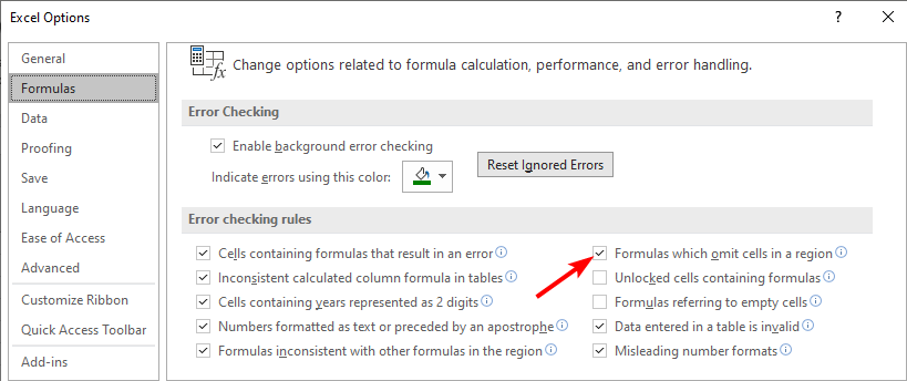
To do it, go to File >> Options >> Formulas.
On the right side, under Error checking rules uncheck the field called Formulas which omit cells in a region.
After you make this change, Excel will stop irritating you with this error message.
Источник
Formula Omits Adjacent Cells Error in Excel: How to Fix It
Ignore the Excel error or update your formula to include the cells

- The error formula omits adjacent cells means that Excel cannot calculate the formula because it is missing something.
- Excel tries to calculate a formula but only takes into account the values from one cell, ignoring other cells with values needed for the calculation.
- If this happens, it means that you have left out a cell on one side of your formula and need to clean up your sheet.
- Download Restoro PC Repair Tool that comes with Patented Technologies (patent available here) .
- Click Start Scan to find Windows issues that could be causing PC problems.
- Click Repair All to fix issues affecting your computer’s security and performance
- Restoro has been downloaded by 0 readers this month.
If you get an error message saying that your formula omits adjacent cells when you try to enter it, your Excel spreadsheet has probably been modified.
The problem is that when such an error occurs, it can mess up your entire worksheet. You may have to redo all of your calculations from scratch or worse, start over, especially if Excel fails to respond when saving.
What does the error formula omits adjacent cells mean in excel?
The error formula omits adjacent cells means that there is an error in the formula in the cell. When you have an array of formulas, Excel assumes that the data for all are continuous and not separated by other data.
If your data is separated by other data or if some cells contain blank values, then Excel will not be able to evaluate the formula correctly. But why does this happen? Below are some possible reasons:
- Cell has no data – The error function in Excel only calculates values for cells where there is data present. If a cell has no data, then it will not be included in the calculation process.
- The cell no longer exists – It is possible that the formula you may be referencing belongs to a cell that has been deleted or renamed.
- Range has been changed – The formula may be referencing a dynamic range that no longer exists due to changes in the spreadsheet.
- Blank cells in between – This error occurs when there are empty cells between each cell that you want to include in your formula.
What can I do if the Excel error formula omits adjacent cells?
Check off the following first before you proceed:
- First, check to make sure that your formula includes all of the necessary parts.
- If you are working with a small data set, try to identify any empty cells and delete them.
1. Uncheck formulas that omit cells
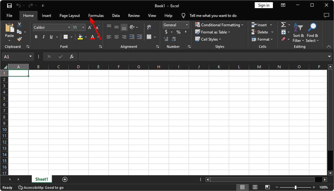
- Launch your Excel sheet and then click on File.
- Navigate to Options and then select Formulas.
- Look for Error checking rules and uncheck Formulas which omit cells in a region.
- Click OK.
2. Switch from absolute to relative reference
- Open the Excel sheet and select the cell that contains the formula.
- Navigate to the formula bar at the top and press F4 until you get the relative reference option.
Absolute and relative references in Excel formulas are two ways to refer to cells in your spreadsheet. They both have their purpose, and sometimes you may find yourself using them interchangeably.
Absolute cell references are the default in Excel. However, there are times when using an absolute reference is not the best option. This type of notation is not always intuitive because it does not take into account the position of the cell that contains the formula.
Read more about this topic
3. Update the formula to include the cells
When you update the formula to include the cells that you want to reference, Excel can properly evaluate it and display its result properly.
The caveat to this method is that if you have a very large spreadsheet with many formulas, then it can be difficult to track down which cell is causing the problem.
If nothing seems to work, you can opt to ignore the error or seek help from the help task pane in Excel. The built-in tool diagnoses some problems and may be able to recommend a solution.
Excel errors are in no shortage as you can expect to encounter a few hiccups when you’re working with sheets and formulas. We have crafted a dedicated article to help you in case you want to recover a corrupted Excel file so that you don’t have to lose all your work.
In other instances, you may be unable to type in Excel, but we know what you can do to keep things moving as you shall see in our expert guide.
Let us know of any other tricks you used if you were in a similar predicament in the comment section below.
Still having issues? Fix them with this tool:
Источник
Adjacent cells omitted warning, why?
LinkBack
Thread Tools
Rate This Thread
Display
Adjacent cells omitted warning, why?
I’m getting the “Formula Omits Adjacent Cells” warning for the following formula on some cells but not others; however everything is working as it should. Why is excel complaining about omitted adjacent cells? It all looks good to me.
I have attached the file I am working on with the hidden rows unhidden so you can see whats going on. It is a weekly football picks spreadsheet that allows you to mark a 1 above the winning teams to get the number of incorrect picks in the left column. If no 1 marks the winning team then the above formula should count the blanks total for that team as 3 and simply assign a 0 incorrect picks for that game. If there is a 1, then the main if formula will tabulate a correct or incorrect pick accordingly.
Last edited by AliGW; 11-18-2019 at 01:58 PM . Reason: Solved tag added — no need to edit thread title or add solved to post. Thanks.
Re: Adjacent cells omitted warning, why?
if you click on the error and select update formula to include cells, it will get rid of the error while keeping the correct value.
You can also fix the first row and then drag down and it will clear the error mark out of the cells.
Last edited by liz5818; 09-11-2013 at 12:31 PM .
Re: Adjacent cells omitted warning, why?
That won’t work because then it tries to add another cell in the calculation that I don’t wan’t. My formula is exactly what I want to do but excel doesn’t like it for some buggy reason.
Last edited by simusphere; 09-11-2013 at 01:29 PM .
Re: Adjacent cells omitted warning, why?
Go to File, Options, Formulas — In the Error Checking rules remove check from «Formulas which omits cells in a region»
If you like my answer please click on * Add Reputation
Don’t forget to mark threads as «Solved» if your problem has been resolved
«Nothing is so firmly believed as what we least know.»
—Michel de Montaigne
Re: Adjacent cells omitted warning, why?
That did the trick AlKey, I’ll mark this as fixed.
Re: [SOLVED] Adjacent cells omitted warning, why?
You’re Welcome. Don’t forget to thank those who helped by clicking on Add Reputation *
Re: Adjacent cells omitted warning, why?
Thank you so much for your answer. I have been living with this annoyance for more years than I want to admit to :/) Like many things in life, we put up with small things that aren’t so big to take the time to fix, but once we do we are overjoyed at the difference. I never thought that there would be anything that could prevent the problem you addressed and today for some reason, I looked it up and got your answer from 3 years ago, and you made my whole day ! ! ! For me I had to go to Tools to get to Options instead of File, Options, but that may be because I’m using a different or older version. Only wanted to point that out in case someone had a similar version as mine. Thank you so much again. In our busy society people could go about their own business and not be concerned about other people’s questions. I have been grateful so many times for those that have cared and answered a question about something I was struggling with, and today I am very grateful for yours.
Thank you again.
Re: [SOLVED] Adjacent cells omitted warning, why?
Big Bird, welcome to the forum and thank you for your feedback

1. Use code tags for VBA. [code] Your Code [/code] (or use the # button)
2. If your question is resolved, mark it SOLVED using the thread tools
3. Click on the star if you think someone helped you
Re: [SOLVED] Adjacent cells omitted warning, why?
I had this problem and realized my formula was using relative referencing (A1) so it was incrementing in each lower cell which was giving me the error in all but the first cell. Once I made the Column static ($A1) and copied it down, the error went away.
I don’t like the idea of shutting off the error checking globally which is, if I understood it correctly, what was suggested.
Источник