
In column A, I have a list of random words, separated by «; «(semicolon & space),
and randomly having 1 to 3 words in each cell.
For example, A1 — A5 would contain the following:
apple
banana; carrot
durian; eggplant
fig
grape; honeydew; icecream
I am trying to surround each word with a specified string. For example, «I eat » before the word,
» everyday.», after the word, which should look like the following in column B.
I eat apple everday.
I eat banana everday.;I eat carrot everday.
I eat durian everday.; I eat eggplant everday.
I eat fig everday.
I eat grape everday.; I eat honeydew everday.; I eat icecream everday.
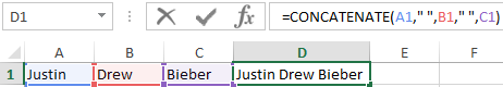
If each cell contains only one word, it would be a simple process of just concatenating:
=CONCATENATE("I eat ",A1," everyday.")
But then when the number of words are random, it starts to get confusing. Of course there is a solution by separating by the semicolons into different columns, add the new string, and add everything together, but I was going for doing it in a single cell.
For the convenience of working with text in Excel, there are text functions. They make it easy to process hundreds of lines at once. Let’s consider some of them on examples.
Examples with TEXT function in Excel
This function converts numbers to string in Excel. Syntax: value (numeric or reference to a cell with a formula that gives a number as a result); Format (to display the number in the form of text).
The most useful feature of the TEXT function is the formatting of numeric data for merging with text data. Excel «doesn’t understand» how to display numbers without using the function. The program just converts them to a basic format.
Let’s see an example. Let’s say you need to combine text in string with numeric values:
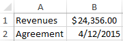
Using an ampersand without a function TEXT produces an inadequate result:
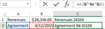
Excel returned the sequence number for the date and the general format instead of the monetary. The TEXT function is used to avoid this. It formats the values according to the user’s request.
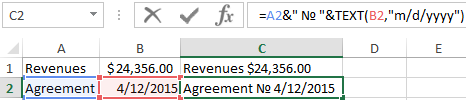
The formula «for a date» now looks like this:
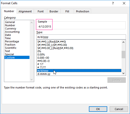
The second argument to the function is the format. Where to take the format line? Right-click on the cell with the value. Click on «Format Cells». In the opened window select «Custom». Copy the required «Type:» in the line. We paste the copied value in the formula.
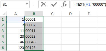
Let’s consider another example where this function can be useful. Add zeros at the beginning of the number. Excel will delete them if you enter it manually. Therefore, we introduce the formula:
If you want to return the old numeric values (without zeros), then use the «—» operator:
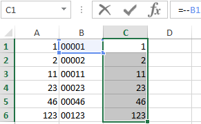
Note that the values are now displayed in numerical format.
Text splitting function in Excel
Individual functions and their combinations allow you to distribute words from one cell to separate cells:
- LEFT (Text, number of characters) displays the specified number of characters from the beginning of the cell;
- RIGHT (Text, number of characters) returns a specified number of characters from the end of the cell;
- SEARCH (Search text, range to search, start position) shows the position of the first occurrence of the searched character or line while viewing from left to right.
The line takes into account the position of each character when dividing the text. Spaces show the beginning or the end of the name you are looking for.
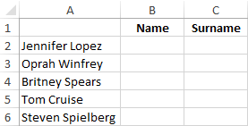
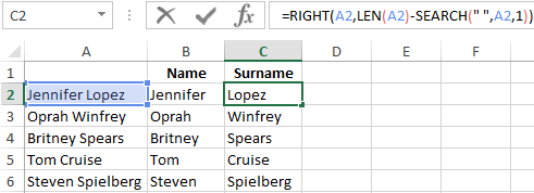
We will split the name, surname and patronymic name into different columns using the functions.
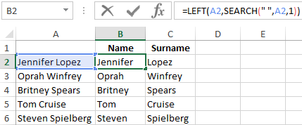
The first line contains only the first and last names separated by a space. Formula for retrieving the name:
The function SEARCH is used to determine the second argument of the LEFT function (the number of characters). It finds a space in cell A2 starting from the left.
For a name, we use the same formula:
Excel determines the number of characters for the RIGHT function using the SEARCH function. The LEN function «counts» the total length of the text. Then the number of characters up to the first space (found by SEARCH) is subtracted.
The formula for extracting the surname:
Next formulas for extracting the surname is a bit different:
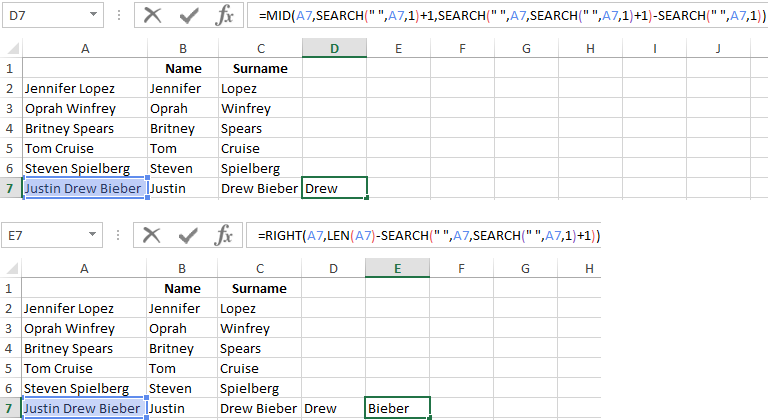
These are five signs on the right. Embedded SEARCH functions search for the second and third spaces in a string. SEARCH («»;A7;1) finds the first space on the left (before the patronymic name). Add one (+1) to the result. We get the position with which we will search for the second space.
Part of the formula SEARCH(» «;A7;SEARCH(» «;A7;1)+1) finds the second space. This will be the final position of the patronymic.
Then the number of characters from the beginning of the line to the second space is subtracted from the total length of the line. The result is the number of characters to the right that you need to return.
Function for merging text in Excel
Use the ampersand (&) operator or the CONCATENATE function to combine values from several cells into one line.
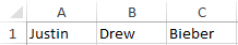
For example, the values are located in different columns (cells):
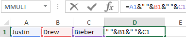
Put the cursor in the cell where the combined three values will be. Enter «=». Select the first cell and click on the keyboard «&» sign. Then enter the space character enclosed in quotation marks (» «). Enter again «&». Therefore, sequentially connect cells with symbols and spaces.
We get the combined values in one cell:
Using the CONCATENATE function:
You can add any sign or string to the final expression using quotation marks in the formula.
Text SEARCH function in Excel
The SEARCH function returns the starting position of the searched text (not case sensitive). For example:
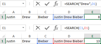
The SEARCH returned to position 8 because the word «Drew» begins with the tenth character in the line. Where can this be useful?
The SEARCH function determines the position of the character in the string line. And the MID function returns symbols values (see the example above). Alternatively, you can replace the found text with the REPLACE.
Download example TEXT functions
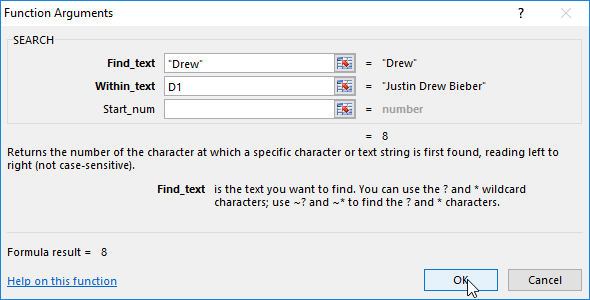
The syntax of the SEARCH function:
- «Find_text» is what you need to find;
- «Withing_text» is where to look;
- «Start_num» is from which position to start searching (by default it is 1).
Use the FIND if you need to take into account the case (lower and upper).
Содержание
- Add text strings at the beginning, at the end, or at another position in Excel cells
- Before you begin, add Add Characters to Excel
- How to add characters at the beginning of cells
- How to add characters at the end of cells
- How to add characters in the middle of cells
- How to add characters before or after specific text in cells
- Set options for adding characters to cells
- How to add text or character to every cell in Excel
- Excel formulas to add text/character to cell
- Concatenation operator
- CONCATENATE function
- CONCAT function
- How to add text to the beginning of cells
- How to add text to the end of cells in Excel
- Add characters to beginning and end of a string
- Combine text from two or more cells
- How to add special character to cell in Excel
- How to add text to formula in Excel
- How to insert text after Nth character
- How to add text before/after a specific character
- Add text after specific character
- Insert text before specific character
- How to add space between text in Excel cell
- How to add the same text to existing cells with VBA
- Prepend text to beginning
- Append text to end
- Add text or character to multiple cells with Ultimate Suite
Add text strings at the beginning, at the end, or at another position in Excel cells
When you need to insert some text into each Excel cell, creating functions or using VBA can be quite time consuming. It gets even more complicated if you need, for example, to add text into a specific position in a cell or before specific text.
The Add Characters feature helps add custom substrings (letters, numbers, spaces, commas or any other characters) to cells in seconds:
Before you begin, add Add Characters to Excel
Add Characters is one of the 20+ features within XLTools Add-in for Excel. Works in Excel 2019, 2016, 2013, 2010, desktop Office 365.

How to add characters at the beginning of cells
Click the Data Cleaning button on XLTools ribbon ![]() Select Add characters from the drop-down list
Select Add characters from the drop-down list ![]() A dialogue box will open.
A dialogue box will open.
Select the range where you want to add characters.

Type the substring you want to add to each cell.
Choose the position in a cell: at the beginning .
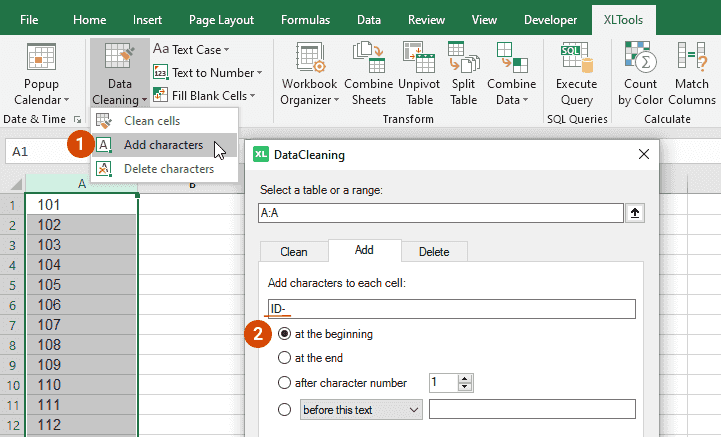
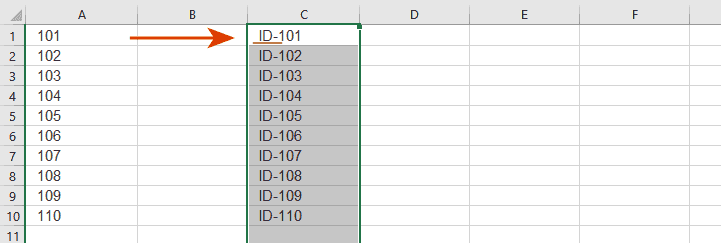
Click OK ![]() Done, the text string is added at the beginning of each cell.
Done, the text string is added at the beginning of each cell.
How to add characters at the end of cells
Click the Data Cleaning button on XLTools ribbon ![]() Select Add characters from the drop-down list
Select Add characters from the drop-down list ![]() A dialogue box will open.
A dialogue box will open.
Select the range where you want to add characters.
Type the substring you want to add to each cell.
Choose the position in a cell: at the end .
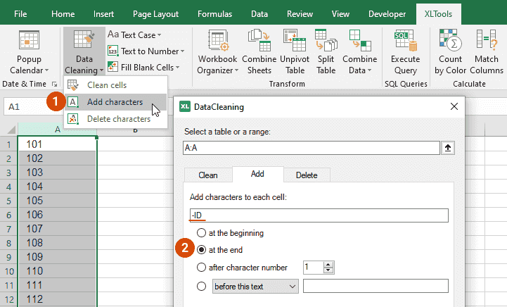
Click OK ![]() Done, the text string is added at the end of each cell.
Done, the text string is added at the end of each cell.
How to add characters in the middle of cells
Click the Data Cleaning button on XLTools ribbon ![]() Select Add characters from the drop-down list
Select Add characters from the drop-down list ![]() A dialogue box will open.
A dialogue box will open.
Select the range where you want to add characters.
Type the substring you want to add to each cell.
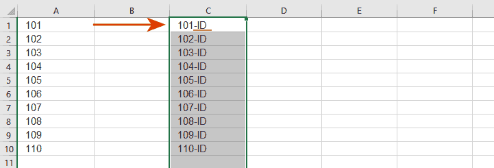
Choose the position in a cell: after character number N ![]() Specify the number of characters from the beginning, where you want to insert the text string.
Specify the number of characters from the beginning, where you want to insert the text string.
Click OK ![]() Done, the text string is added in the middle of each cell.
Done, the text string is added in the middle of each cell.
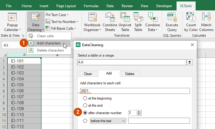
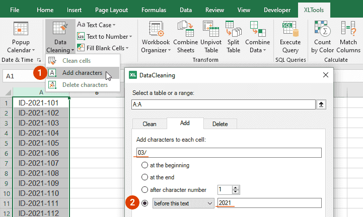
How to add characters before or after specific text in cells
Click the Data Cleaning button on XLTools ribbon ![]() Select Add characters from the drop-down list
Select Add characters from the drop-down list ![]() A dialogue box will open.
A dialogue box will open.
Select the range where you want to add characters.
Type the substring you want to add to each cell.
Choose the position in a cell: before this tex t or after this text ![]() Type the text string to search for (case sensitive by default).
Type the text string to search for (case sensitive by default).
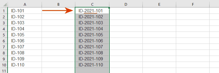
Click OK ![]() Done, the text string is added before or after the specified text in those cells, where it was found.
Done, the text string is added before or after the specified text in those cells, where it was found.
Set options for adding characters to cells
By default, the Add Characters feature does not process cells that contain formulas, not to interfere with calculations. You can specify additional data processing options:
Check the Skip empty cells option
Select this option, if you don’t want to add the characters into empty (blank) cells.
Check the Skip non-text cells option
Select this option, if you want to process only cells with text. All cells that have number, date, currency or other format will be ignored.
Check the Skip header row option
Select this option, if you want to ignore the first row with the table header.
Источник
How to add text or character to every cell in Excel
 by Svetlana Cheusheva, updated on March 10, 2023
Wondering how to add text to an existing cell in Excel? In this article, you will learn a few really simple ways to insert characters in any position in a cell.
When working with text data in Excel, you may sometimes need to add the same text to existing cells to make things clearer. For example, you might want to put some prefix at the beginning of each cell, insert a special symbol at the end, or place certain text before a formula.
I guess everyone knows how to do this manually. This tutorial will teach you how to quickly add strings to multiple cells using formulas and automate the work with VBA or a special Add Text tool.
Excel formulas to add text/character to cell
To add a specific character or text to an Excel cell, simply concatenate a string and a cell reference by using one of the following methods.
Concatenation operator
The easiest way to add a text string to a cell is to use an ampersand character (&), which is the concatenation operator in Excel.
This works in all versions of Excel 2007 — Excel 365.
CONCATENATE function
The same result can be achieved with the help of the CONCATENATE function:
The function is available in Excel for Microsoft 365, Excel 2019 — 2007.
CONCAT function
To add text to cells in Excel 365, Excel 2019, and Excel Online, you can use the CONCAT function, which is a modern replacement of CONCATENATE:
Note. Please pay attention that, in all formulas, text should be enclosed in quotation marks.
These are the general approaches, and the below examples show how to apply them in practice.
How to add text to the beginning of cells
To add certain text or character to the beginning of a cell, here’s what you need to do:
- In the cell where you want to output the result, type the equals sign (=).
- Type the desired text inside the quotation marks.
- Type an ampersand symbol (&).
- Select the cell to which the text shall be added, and press Enter .
Alternatively, you can supply your text string and cell reference as input parameters to the CONCATENATE or CONCAT function.
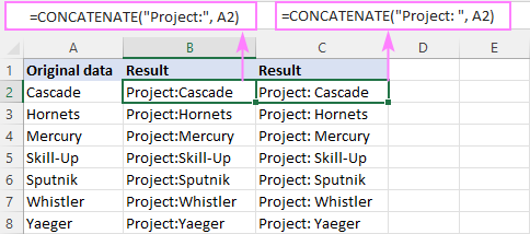
For example, to prepend the text «Project:» to a project name in A2, any of the below formulas will work.
In all Excel versions:
In Excel 365 and Excel 2019:
Enter the formula in B2, drag it down the column, and you will have the same text inserted in all cells.
Tip. The above formulas join two strings without spaces. To separate values with a whitespace, type a space character at the end of the prepended text (e.g. «Project: «).
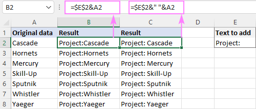
For convenience, you can input the target text in a predefined cell (E2) and add two text cells together:
Please notice that the address of the cell containing the prepended text is locked with the $ sign, so that it won’t shift when copying the formula down.
With this approach, you can easily change the added text in one place, without having to update every formula.
How to add text to the end of cells in Excel
To append text or specific character to an existing cell, make use of the concatenation method again. The difference is in the order of the concatenated values: a cell reference is followed by a text string.
For instance, to add the string «-US» to the end of cell A2, these are the formulas to use:
Alternatively, you can enter the text in some cell, and then join two cells with text together:
Please remember to use an absolute reference for the appended text ($D$2) for the formula to copy correctly across the column.

Add characters to beginning and end of a string
Knowing how to prepend and append text to an existing cell, there is nothing that would prevent you from using both techniques within one formula.
As an example, let’s add the string «Project:» to the beginning and «-US» to the end of the existing text in A2.
=CONCATENATE(«Project:», A2, «-US»)
=CONCAT(«Project:», A2, «-US»)
With the strings input in separate cells, this works equally well:

Combine text from two or more cells
To place values from multiple cells into one cell, concatenate the original cells by using the already familiar techniques: an ampersand symbol, CONCATENATE or CONCAT function.
For example, to combine values from columns A and B using a comma and a space («, «) for the delimiter, enter one of the below formulas in B2, and then drag it down the column.
Add text from two cells with an ampersand:
Combine text from two cells with CONCAT or CONCATENATE:
When adding text from two columns, be sure to use relative cell references (like A2), so they adjust correctly for each row where the formula is copied.

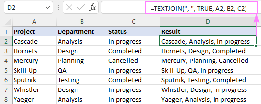
To combine text from multiple cells in Excel 365 and Excel 2019, you can leverage the TEXTJOIN function. Its syntax provides for a delimiter (the first argument), which makes the formular more compact and easier to manage.
For example, to add strings from three columns (A, B and C), separating the values with a comma and a space, the formula is:
=TEXTJOIN(«, «, TRUE, A2, B2, C2)
How to add special character to cell in Excel
To insert a special character in an Excel cell, you need to know its code in the ASCII system. Once the code is established, supply it to the CHAR function to return a corresponding character. The CHAR function accepts any number from 1 to 255. A list of printable character codes (values from 32 to 255) can be found here.
To add a special character to an existing value or a formula result, you can apply any concatenation method that you like best.
For example, to add the trademark symbol (в„ў) to text in A2, any of the following formulas will work:

How to add text to formula in Excel
To add a certain character or text to a formula result, just concatenate a string with the formula itself.
Let’s say, you are using this formula to return the current time:
=TEXT(NOW(), «h:mm AM/PM»)
To explain to your users what time that is, you can place some text before and/or after the formula.
Insert text before formula:
=»Current time: «&TEXT(NOW(), «h:mm AM/PM»)
=CONCATENATE(«Current time: «, TEXT(NOW(), «h:mm AM/PM»))
=CONCAT(«Current time: «, TEXT(NOW(), «h:mm AM/PM»))

Add text after formula:
=TEXT(NOW(), «h:mm AM/PM»)&» — current time»
=CONCATENATE(TEXT(NOW(), «h:mm AM/PM»), » — current time»)
=CONCAT(TEXT(NOW(), «h:mm AM/PM»), » — current time»)

Add text to formula on both sides:
=»It’s » &TEXT(NOW(), «h:mm AM/PM»)& » here in Gomel»
=CONCATENATE(«It’s «, TEXT(NOW(), «h:mm AM/PM»), » here in Gomel»)
=CONCAT(«It’s «, TEXT(NOW(), «h:mm AM/PM»), » here in Gomel»)

How to insert text after Nth character
To add a certain text or character at a certain position in a cell, you need to split the original string into two parts and place the text in between. Here’s how:
- Extract a substring preceding the inserted text with the help of the LEFT function:
LEFT(cell, n) - Extract a substring following the text using the combination of RIGHT and LEN:
RIGHT(cell, LEN(cell) -n) - Concatenate the two substrings and the text/character using an ampersand symbol.
The complete formula takes this form:
The same parts can be joined together by using the CONCATENATE or CONCAT function:
The task can also be accomplished by using the REPLACE function:
The trick is that the num_chars argument that defines how many characters to replace is set to 0, so the formula actually inserts text at the specified position in a cell without replacing anything. The position (start_num argument) is calculated using this expression: n+1. We add 1 to the position of the nth character because the text should be inserted after it.
For example, to insert a hyphen (-) after the 2 nd character in A2, the formula in B2 is:
=LEFT(A2, 2) &»-«& RIGHT(A2, LEN(A2) -2)
=CONCATENATE(LEFT(A2, 2), «-«, RIGHT(A2, LEN(A2) -2))
Drag the formula down, and you will have the same character inserted in all the cells:

How to add text before/after a specific character
To insert certain text before or after a particular character, you need to determine the position of that character in a string. This can be done with the help of the SEARCH function:
Once the position is determined, you can add a string exactly at that place by using the approaches discussed in the above example.
Add text after specific character
To insert some text after a given character, the generic formula is:
For instance, to insert the text (US) after a hyphen in A2, the formula is:
=LEFT(A2, SEARCH(«-«, A2)) &»(US)»& RIGHT(A2, LEN(A2) — SEARCH(«-«, A2))
=CONCATENATE(LEFT(A2, SEARCH(«-«, A2)), «(US)», RIGHT(A2, LEN(A2) -SEARCH(«-«, A2)))

Insert text before specific character
To add some text before a certain character, the formula is:
As you see, the formulas are very similar to those that insert text after a character. The difference is that we subtract 1 from the result of the first SEARCH to force the LEFT function to leave out the character after which the text is added. To the result of the second SEARCH, we add 1, so that the RIGHT function will fetch that character.
For example, to place the text (US) before a hyphen in A2, this is the formula to use:
=LEFT(A2, SEARCH(«-«, A2) -1) &»(US)»& RIGHT(A2, LEN(A2) -SEARCH(«-«, A2) +1)
=CONCATENATE(LEFT(A2, SEARCH(«-«, A2) -1), «(US)», RIGHT(A2, LEN(A2) -SEARCH(«-«, A2) +1))

- If the original cell contains multiple occurrences of a character, the text will be inserted before/after the first occurrence.
- The SEARCH function is case-insensitive and cannot distinguish lowercase and uppercase characters. If you aim to add text before/after a lowercase or uppercase letter, then use the case-sensitive FIND function to locate that letter.
How to add space between text in Excel cell
In fact, it is just a specific case of the two previous examples.
To add space at the same position in all cells, use the formula to insert text after nth character, where text is the space character (» «).
For example, to insert a space after the 10 th character in cells A2:A7, enter the below formula in B2 and drag it through B7:
=LEFT(A2, 10) &» «& RIGHT(A2, LEN(A2) -10)
=CONCATENATE(LEFT(A2, 10), » «, RIGHT(A2, LEN(A2) -10))
In all the original cells, the 10 th character is a colon (:), so a space is inserted exactly where we need it:

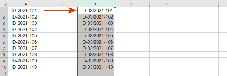
To insert space at a different position in each cell, adjust the formula that adds text before/after a specific character.
In the sample table below, a colon (:) is positioned after the project number, which may contain a variable number of characters. As we wish to add a space after the colon, we locate its position using the SEARCH function:
=LEFT(A2, SEARCH(«:», A2)) &» «& RIGHT(A2, LEN(A2)-SEARCH(«:», A2))
=CONCATENATE(LEFT(A2, SEARCH(«:», A2)), » «, RIGHT(A2, LEN(A2)-SEARCH(«:», A2)))

How to add the same text to existing cells with VBA
If you often need to insert the same text in multiple cells, you can automate the task with VBA.
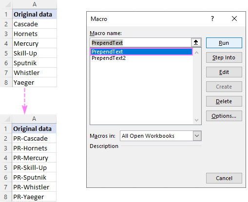
Prepend text to beginning
The below macros add text or a specific character to the beginning of all selected cells. Both codes rely on the same logic: check each cell in the selected range and if the cell is not empty, prepend the specified text. The difference is where the result is placed: the first code makes changes to the original data while the second one places the results in a column to the right of the selected range.
If you have little experience with VBA, this step-by-step guide will walk you through the process: How to insert and run VBA code in Excel.
Macro 1: adds text to the original cells
This code inserts the substring «PR-» to the left of an existing text. Before using the code in your worksheet, be sure to replace our sample text with the one you really need.
Macro 2: places the results in the adjacent column
Before running this macro, make sure there is an empty column to the right of the selected range, otherwise the existing data will be overwritten.

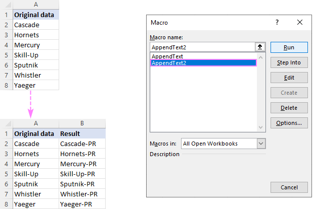
Append text to end
If you are looking to add a specific string/character to the end of all selected cells, these codes will help you get the work done quickly.
Macro 1: appends text to the original cells
Our sample code inserts the substring «-PR» to the right of an existing text. Naturally, you can change it to whatever text/character you need.

Macro 2: places the results in another column
This code places the results in a neighboring column. So, before you run it, make certain you have at least one empty column to the right of the selected range, otherwise your existing data will be overwritten.
Add text or character to multiple cells with Ultimate Suite
In the first part of this tutorial, you’ve learned a handful of different formulas to add text to Excel cells. Now, let’s me show you how to accomplish the task with a few clicks 🙂
With Ultimate Suite installed in your Excel, here are the steps to follow:
- Select your source data.
- On the Ablebits tab, in the Text group, click Add.
- On the Add Text pane, type the character/text you wish to add to the selected cells, and specify where it should be inserted:
- At the beginning
- At the end
- Before specific text/character
- After specific text/character
- After Nth character from the beginning or end
- Click the Add Text button. Done!
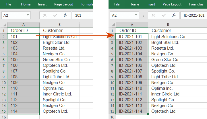
As an example, let’s insert the string «PR-» after the «-» character in cells A2:A7. For this, we configure the following settings:
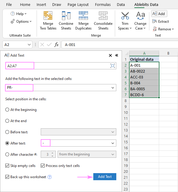
A moment later, we get the desired result:

These are the best ways to add characters and text strings in Excel. I thank you for reading and hope to see you on our blog next week!
Источник
1st option:
="The next to die will be "& A2 & ' '& B2 & ". Cheers!"
2nd option:
(for hardcore users)
Create your own function:
Function myString(ParamArray Vals() As Variant)
    Separator1 = "{"
    Separator2 = "}"
    finalString = ""
    initialString = Vals(0)
    found = True
    firstpos = 1
    While found = True
        pos = InStr(firstpos, initialString, Separator1)
        If pos = 0 Then
            found = False
            endpartval = Mid(initialString, firstpos)
            finalString = finalString + endpartval
        Else
            stringParts = Mid(initialString, firstpos, pos - firstpos)
            pos1 = InStr(pos, initialString, Separator2)
            firstpos = pos1 + 1
            varNumber = Mid(initialString, pos + 1, pos1 - pos - 1)
            finalString = finalString + stringParts + Vals(varNumber + 1)
        End If
    Wend
    myString = finalString
End Function
To make it work you have to open VBA/Macros with ALT+ F11, then under ThisWorkbook insert a new module and paste the code.
Now, in any cell you can put
=mystring("The next to die will be {0} {1}. Cheers!",A2,B2)
or whatever. Keep in mind that the string must go first and then the cell references.
This is valid:
=mystring("The next to die will be {0}, {3} and {2}. Cheers!",A2,B2,B3)
This isn’t:
=mystring(A2,"The next to die will be {0}, {3} and {2}. Cheers!",B2,B3)
In Excel, there are multiple string (text) functions that can help you to deal with textual data. These functions can help you to change a text, change the case, find a string, count the length of the string, etc. In this post, we have covered top text functions. (Sample Files)
1. LEN Function
LEN function returns the count of characters in the value. In simple words, with the LEN function, you can count how many characters are there in value. You can refer to a cell or insert the value in the function directly.
Syntax
LEN(text)
Arguments
- text: A string for which you want to count the characters.
Example
In the below example, we have used the LEN to count letters in a cell. “Hello, World” has 10 characters with a space between and we have got 11 in the result.

In the below example, “22-Jan-2016” has 11 characters, but LEN returns 5.

The reason behind it is that the LEN function counts the characters in the value of a cell and is not concerned with formatting.
Related: How to COUNT Words in Excel
2. FIND Function
FIND function returns a number which is the starting position of a substring in a string. In simple words, by using the find function you can find (case sensitive) a string’s starting position from another string.
Syntax
FIND(find_text,within_text,[start_num])
Arguments
- find_text: The text which you want to find from another text.
- within_text: The text from which you want to locate the text.
- [start_num]: The number represents the starting position of the search.
Example
In the below example, we have used the FIND to locate the “:” and then with the help of MID and LEN, we have extracted the name from the cell.
3. SEARCH Function
SEARCH function returns a number which is the starting position of a substring in a string. In simple words, with the SEARCH function, you can search (non-case sensitive) for a text string’s starting position from another string.
Syntax
SEARCH(find_text,within_text,[start_num])
Arguments
- find_text: A text which you want to find from another text.
- within_text: A text from which you want to locate the text. You can refer to a cell, or you can input a text in your function.
Example
In the below example, we are searching for the alphabet “P” and we have specified start_num as 1 to start our search. Our formula returns 1 as the position of the text.

But, if you look at the word, we also have a “P” in the 6th position. That means the SEARCH function can only return the position of the first occurrence of a text, or if you specify the start position accordingly.
4. LEFT Function
LEFT Functions return sequential characters from a string starting from the left side (starting). In simple words, with the LEFT function, you can extract characters from a string from its left side.
Syntax
LEFT(text,num_chars)
Arguments
- text: A text or number from which you want to extract characters.
- [num_char]: The number of characters you want to extract.
Example
In the below example, we have extracted the first five digits from a text string using LEFT by specifying the number of characters to extract.

In the below example, we have used LEN and FIND along with the LEFT to create a formula that extracts the name from the cell.

5. RIGHT Function
The RIGHT function returns sequential characters from a string starting from the right side (ending). In simple words, with the RIGHT function, you can extract characters from a string from its left side.
Syntax
RIGHT(text,num_chars)
Arguments
- text: A text or number from which you want to extract characters.
- [num_char]: A number of characters you want to extract.
Example
In the below example, we have extracted 6 characters using the right function. If you know, how many characters you need to extract from the string, you can simply extract them by using a number.

Now, if you look at the below example, where we have to extract the last name from the cell, but we are not confirmed about the number of characters in the last name.

So, we are using LEN and FIND to get the name. Let me show you how we have done this.
First of all, we have used the LEN to get the length of that entire text string, then we used the FIND to get the position number of space between first and last names. And in the end, we have used both the figures to get the last name.
Arguments
- value1: A cell reference, an array, or a number that is directly entered into the function.
- [value2]: A cell reference, an array, or a number that is directly entered into the function.
6. MID Function
MID returns a substring from a string using a specific position and number of characters. In simple words, with MID, you can extract a substring from a string by specifying the starting character and number of characters you want to extract.
Syntax
MID(text,start_num,num_chars)
Arguments
- text: A text or a number from which you want to extract characters.
- start_char: A number for the position of the character from where you want to extract characters.
- num_chars: The number of characters you want to extract from the start_char.
Example
In the below example, we have used different values:
- From the 6th character to the next 6 characters.
- From the 6th character to the next 10 characters.
- We have used starting a character in negative and it has returned an error.
- By using 0 for the number of characters to extract and it has returned a blank.
- With a negative number for the number of characters to extract and it has returned an error.
- The starting number is zero and it has returned an error.
- Text string directly into the function.

7. LOWER Function
LOWER returns the string after converting all the letters in small. In simple words, it converts a text string where all the letters you have are in small letters, numbers will stay intact.
Syntax
LOWER(text)
Arguments
- text: The text which you want to convert to the lowercase.
Example
In the below example, we have compared the lower case, upper case, proper case, and sentence case with each other.

A lower case text has all the letters in a small case compared to others.
8. PROPER Function
The PROPER function returns the text string into a proper case. In simple words, with a PROPER function where the first letter of the word is in capital and rest in small (proper case).
Syntax
PROPER(text)
Arguments
- text: The text which you want to convert to the proper case.
Example
In the below example, we have a proper case that has the first letter in the capital case in a word and the rest of the letters are in the lower case compared to the other two cases lowercase and uppercase.

In the below example, we have used the PROPER function to streamline first name and last name into the proper case.

9. UPPER Function
The UPPER function returns the string after converting all the letters in the capital. In simple words, it converts a text string where all the letters you have are in capital form and numbers will stay intact.
Syntax
UPPER(text)
Arguments
- text: The text which you want to convert into uppercase.
Example
In the below example, we have used the UPPER to convert name text to capital letters from the text in which characters are in different cases.

10. REPT Function
REPT function returns a text value several times. In simple words, with the REPT function, you can specify a text, and a number to repeat that text.
Syntax
REPT(value1, [value2], …)
Example
In the below example, we have used different type of text for repetition using REPT. It can repeat any type of text or numbers and even symbols that you specify in function and the main use of the REPT function is for creating in-cell charts.
