
In this article, we will learn How to add cells in Excel.
Scenario :
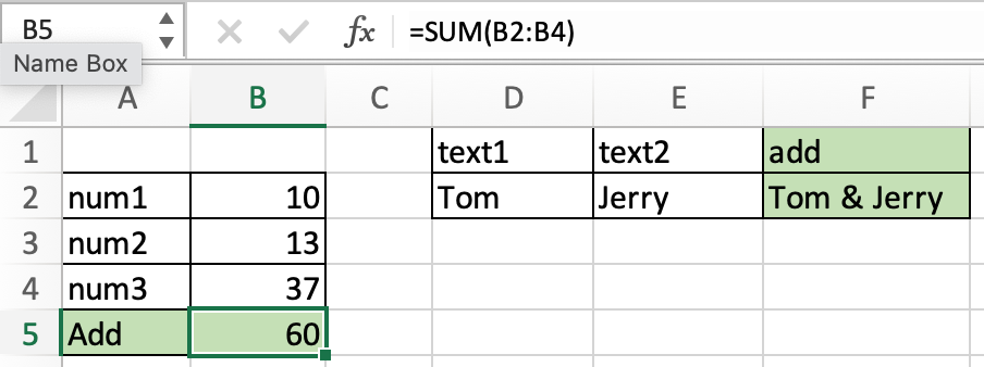
Excel Add cells. Adding means two different things in excel either adding number values or joining text values. For example finding the sum of sales of a product. To add numbers we use the SUM function to directly add values or use + operator with numbers or cell references. For example Joining the First name and Last name into one cell with space. To join or combine two texts we use CONCATENATE function or & operator with text values or cell references. Let’s learn how to add cells in excel using both methods and sample data calculation to illustrate the usage.
Add number cells in Excel
To add numbers cells in excel using cell references you can use either of the two methods mentioned below.
- =SUM(A1, A2, A3) or =SUM(A1:A3).
- =A1 + A2 + A3
Add text cells in Excel
To add text cells in excel using cell references you can use either of the two methods mentioned below.
- =CONCATENATE(A2, B2, C2)
- =A2 & B2 & C2
Example :
All of these might be confusing to understand. Let’s understand how to use the function using an example. Here we have sample data to sum. And we need to add D2, D3, D4 cells. Just go to any cell and use the formula for the required cells.
Use the formula:
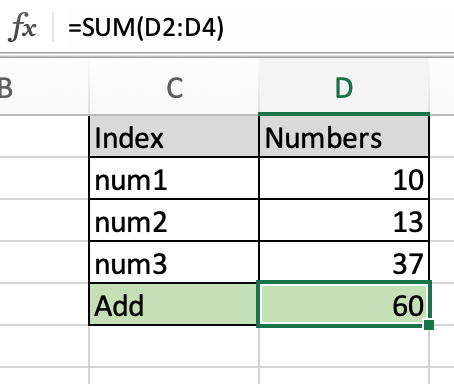
As you can see the sum of values in the D5 cell. You can use conditional summing using SUMIF or SUMIFS function.
Add two text cells in Excel
Here we are given two names and we need to add them to make a name out of it. Here the result expected is Tom & Jerry. To combine the two values
Use the formula:
=CONCATENATE(D2,» & «,E2) or =D2&» & «&E2
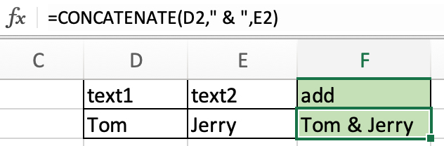
As you can see clearly the two cells are added in the new cell. Using the cell reference in excel. Use the TEXTJOIN function in Excel 365 (newer version) to add texts in excel directly.
Here are all the observational notes using the formula in Excel.
Notes :
- + and & are operators to add numbers or cells.
- Use cell reference wherever possible inplace of giving manual input in a formula.
Hope this article about How to add cells in Excel is explanatory. Find more articles on calculating values and related Excel formulas here. If you liked our blogs, share it with your friends on Facebook. And also you can follow us on Twitter and Facebook. We would love to hear from you, do let us know how we can improve, complement or innovate our work and make it better for you. Write to us at info@exceltip.com.
Related Articles :
Relative and Absolute Reference in Excel : Understanding of Relative and Absolute Reference in Excel is very important to work effectively on Excel. Relative and Absolute referencing of cells and ranges.
How to use the SUMPRODUCT function in Excel : Returns the SUM after multiplication of values in multiple arrays in excel.
SUM if date is between : Returns the SUM of values between given dates or period in excel.
Sum if date is greater than given date : Returns the SUM of values after the given date or period in excel.
2 Ways to Sum by Month in Excel : Returns the SUM of values within a given specific month in excel.
How to Sum Multiple Columns with Condition : Returns the SUM of values across multiple columns having condition in excel.
How to use wildcards in excel : Count cells matching phrases using the wildcards in excel.
How to Insert Row Shortcut in Excel : Use Ctrl + Shift + = to open the Insert dialog box where you can insert row, column or cells in Excel.
Popular Articles :
50 Excel Shortcuts to Increase Your Productivity : Get faster at your tasks in Excel. These shortcuts will help you increase your work efficiency in Excel.
How to use the IF Function in Excel : The IF statement in Excel checks the condition and returns a specific value if the condition is TRUE or returns another specific value if FALSE.
How to use the VLOOKUP Function in Excel : This is one of the most used and popular functions of excel that is used to lookup value from different ranges and sheets.
How to use the SUMIF Function in Excel : This is another dashboard essential function. This helps you sum up values on specific conditions.
How to use the COUNTIF Function in Excel : Count values with conditions using this amazing function. You don’t need to filter your data to count specific values. Countif function is essential to prepare your dashboard.
There may be instances where you need to add the same text to all cells in a column. You might need to add a particular title before names in a list, or a particular symbol at the end of the text in every cell.
The good thing is you don’t need to do this manually.
Excel provides some really simple ways in which you can add text to the beginning and/ or end of the text in a range of cells.
In this tutorial we will see 4 ways to do this:
- Using the ampersand operator (&)
- Using the CONCATENATE function
- Using the Flash Fill feature
- Using VBA
So let’s get started!
Method 1: Using the ampersand Operator
An ampersand (&) can be used to easily combine text strings in Excel. Let’s see how you use it to add text at the beginning or end or both in Excel.
Using the ampersand Operator to Add Text to the Beginning of all Cells
The ampersand (&) is an operator that is mainly used to join several text strings into one.
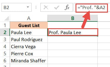
Here’s how you can use it to add text to the beginning of all cells in a range. Let us assume you have the following list of names and want to add the title “Prof.” before every name:

Below are the steps to add a text before a text string in Excel:
- Click on the first cell of the column where you want the converted names to appear (B2).
- Type equal sign (=), followed by the text “Prof. “, followed by an ampersand (&).
- Select the cell containing the first name (A2).
- Press the Return Key.
- You will notice that the title “Prof.” is added before the first name in the list.

- It’s now time to copy this formula to the rest of the cells in the column. Simply double click the fill handle (located at the bottom right of cell B2). Alternatively, you can drag down the fill handle to achieve the same effect.
That’s it, all your cells in column B should now contain the title “Prof.” preceding each name.

Using the ampersand Operator to Add Text to the End of all Cells
Now let us see how to add some text to the end of every name in the dataset. Let us say you want to add the text “(MD)” at the end of every name. In that case, here are the steps you need to follow:
- Click on the first cell of the column where you want the converted names to appear (C2 in our case).
- Type equal sign (=)
- Select the cell containing the first name (B2 in our case).
- Next, insert an ampersand (&), followed by the text “ (MD)”.
- Press the Return Key.
- You will notice that the text “(MD).” added after the first name in the list.

- It’s now time to copy this formula to the rest of the cells in the column. Simply double click the fill handle (located at the bottom right of cell C2). Alternatively, you can drag down the fill handle to achieve the same effect.

All your cells in column C should now contain the text “(MD”) at the end of each name.

Method 2: Using the CONCATENATE Function
CONCATENATE is an Excel function that you can use to add text at the beginning and end of the text string.
Let’s see how to use CONCATENATE to do this.
Using CONCATENATE to Add Text to the Beginning of all Cells
The CONCATENATE() function provides the same functionality as the ampersand (&) operator. The only difference is in the way both are used.
The general syntax for the CONCATENATE function is:
=CONCATENATE(text1, [text2], …)
Where text1, text2, etc. are substrings that you want to combine together.
Let’s apply the CONCATENATE function to the same dataset as above:
- Click on the first cell of the column where you want the converted names to appear (B2).
- Type equal sign (=).
- Enter the function CONCATENATE, followed by an opening bracket (.
- Type the title “Prof. ” in double-quotes, followed by a comma (,).
- Select the cell containing the first name (A2)
- Place a closing bracket. In our example, your formula should now be: =CONCATENATE(“Prof. “,A2).
- Press the Return Key.
- You will notice that the title “Prof.” is added before the first name on the list.

- It’s now time to copy this formula to the rest of the cells in the column. Simply double click the fill handle (located at the bottom right of cell B2). Alternatively, you can drag down the fill handle to achieve the same effect.

That’s it, all your cells in column B should now contain the title “Prof.” preceding each name.

Using CONCATENATE to Add Text to the End of all Cells
Now let us see how to add some text to the end of every name in the dataset. Let us say you want to add the text “(MD)” at the end of every name. In that case, here are the steps you need to follow:
- Click on the first cell of the column where you want the converted names to appear (C2 in our example).
- Type equal sign (=).
- Enter the function CONCATENATE, followed by an opening bracket (.
- Select the cell containing the first name (B2 in our example).
- Next, insert a comma, followed by the text “ (MD)”.
- Place a closing bracket. In our example, your formula should now be: =CONCATENATE(B2,” (MD)”).
- Press the Return Key.
- You will notice that the text “(MD).” added after the first name in the list.

- It’s now time to copy this formula to the rest of the cells in the column. Simply double click the fill handle (located at the bottom right of cell C2).

All your cells in column C should now contain the text “(MD”) at the end of each name.

Notice that since you’re using a formula, your column C depends on columns A and B. So if you make any changes to the original values in column A, they get reflected in column C.
If you decide to only retain the converted names and delete columns A and B, you will get an error, as shown below:

To make sure that this does not happen, it’s best to first convert the formula results to permanent values copying them and pasting them as values in the same column (Right-click and select Paste Options->Values from the Popup menu).

Now you can go ahead and delete columns A and B if you need to.
Also read: How to Remove First Character in Excel?
Method 3: Using the Flash Fill Feature
Flash fill is a relatively new feature that looks at the pattern of what you are trying to achieve and then does it for all the cells in a column.
You can also use Flash fill to so text manipulation as we will see in the following examples.
Using Flash Fill to Add Text to the Beginning of all Cells
The Excel flash fill feature is like a magical button. It is available if you’re on any Excel version from 2013 onwards.
The feature takes advantage of Excel’s pattern recognition capabilities. It basically recognizes a pattern in your data and automatically fills in the other cells of the column with the same pattern for you.
Here’s how you can use Flash Fill to add text to the beginning of all cells in a column:
- Click on the first cell of the column where you want the converted names to appear (B2).
- Manually type in the text Prof. , followed by the first name of your list.

- Press the Return Key.
- Click on cell B2 again.
- Under the Data tab, click on the Flash Fill button (in the ‘Data Tools’ group). Alternatively, you can just press CTRL+E on your keyboard (Command+E if you’re on a Mac).


This will copy the same pattern to the rest of the cells in the column… in a flash!

Using Flash Fill to Add Text to the End of all Cells in a Column
If you want to add the text “ (MD)” to the end of the names, follow the same steps:
- Click on the first cell of the column where you want the converted names to appear (C2).
- Manually type in or copy the text from column B2 into C2.
- Add the text “(MD)” after that.

- Under the Data tab, click on the Flash Fill or press CTRL+E on your keyboard (Command+E if you’re on a Mac).

That’s all, you get every cell filled in with the same pattern!

We especially like this method because it is simple, quick, and easy. Moreover, since it’s formula-free, the results do not depend on the original columns.
So they remain unchanged even if you delete rows A and B!

Method 4: Using VBA Code
And of course, if you’re comfortable with VBA, you can also add text before or after a text string using it.
Using VBA to Add Text to the Beginning of all Cells in a Column
If coding with VBA does not intimidate you then this method can help get your work done quickly too.
Here’s the code we will be using to add the title “Prof. “ to the beginning of all cells in a range. You can select and copy it:
Sub add_text_to_beginning()
Dim rng As Range
Dim cell As Range
Set rng = Application.Selection
For Each cell In rng
cell.Offset(0, 1).Value = "Prof. " & cell.Value
Next cell
End Sub
Follow these steps to use the above code:
- From the Developer Menu Ribbon, select Visual Basic.
- Once your VBA window opens, Click Insert->Module. Now you can start coding. Type or copy-paste the above lines of code into the module window. Your code is now ready to run.
- Select the range of cells containing the text you want to convert. Make sure the column next to it is blank because this is where the code will display the results.
- Navigate to Developer->Macros-> add_text_to_beginning->Run.
You will now see the converted text next to your selected range of cells.
Note: You can change the text in line 6 from “Prof. ” to whatever text you need to add to the beginning of all cells.
Using VBA to Add Text to the End of all Cells in a Column
Now, what if you want to add text to the end of all the cells, instead of the beginning? This only involves making a tweak to line 6 of the above code. So if you want to add the text “ (MD)” to the end of all cells, change line 6 to:
cell.Offset(0, 1).Value = cell.Value & “ (MD)”
So your full code should now be:
Sub add_text_to_end()
Dim rng As Range
Dim cell As Range
Set rng = Application.Selection
For Each cell In rng
cell.Offset(0, 1).Value = cell.Value & " (MD)"
Next cell
End Sub
Here’s the final result:
You can now delete the first two columns if you need to. Do remember to keep a backup of your sheet, because the results of VBA code are usually irreversible.
Note: You can change the text in line 6 from “ (MD)” to whatever text you need to add to the end of all cells in the range.
In this tutorial, we showed you four ways in which you can add text to the beginning and/ or end of all cells in a range.
There are plenty of other methods that you can find online too, and all of them work just as well as the ones shown here.
You may feel free to choose whatever method suits you, your requirement, and your version of Excel. In the end, what matters is getting what you need to be done quickly and effectively.
Other Excel tutorials you may like:
- How to Remove Text after a Specific Character in Excel
- How to Reverse a Text String in Excel
- How to Count How Many Times a Word Appears in Excel
- How to Remove Commas in Excel (from Numbers or Text String)
- How to Remove a Specific Character from a String in Excel
- How to Change Uppercase to Lowercase in Excel
- How to Separate Address in Excel?
- How to Concatenate with Line Breaks in Excel?
- How to Separate Names in Excel
This post will guide you how to insert character or text in middle of cells in Excel. How do I add text string or character to each cell of a column or range with a formula in Excel. How to add text to the beginning of all selected cells in Excel. How to add character after the first character of cells in Excel.
Assuming that you have a list of data in range B1:B5 that contain string values and you want to add one character “E” after the first character of string in Cells. You can refer to the following two methods.
Table of Contents
- 1. Insert Character or Text to Cells with a Formula
- 2. Insert Character or Text to Cells with VBA
- 3. Video: Insert Character or Text to Cells
- 4. Related Functions
1. Insert Character or Text to Cells with a Formula
To insert the character to cells in Excel, you can use a formula based on the LEFT function and the MID function. Like this:
=LEFT(B1,1) & "E" & MID(B1,2,299)Type this formula into a blank cell, such as: Cell C1, and press Enter key. And then drag the AutoFill Handle down to other cells to apply this formula.
This formula will inert the character “E” after the first character of string in Cells. And if you want to insert the character or text string after the second or third or N position of the string in Cells, you just need to replace the number 1 in Left function and the number 2 in MID function as 2 and 3. Like below:
=LEFT(B1,2) & "E" & MID(B1,3,299)You can also use an Excel VBA Macro to insert one character or text after the first position of the text string in Cells. Just do the following steps:
Step1: open your excel workbook and then click on “Visual Basic” command under DEVELOPER Tab, or just press “ALT+F11” shortcut.

Step2: then the “Visual Basic Editor” window will appear.
Step3: click “Insert” ->”Module” to create a new module.

Step4: paste the below VBA code into the code window. Then clicking “Save” button.
Sub AddCharToCells()
    Dim cel As Range
    Dim curR As Range
    Set curR = Application.Selection
    Set curR = Application.InputBox("select one Range that you want to insert one
    character", "add character to cells", curR.Address, Type: = 8)
    For Each cel In curR
        cel.Value = VBA.Left(cel.Value, 1) & "E" & VBA.Mid(cel.Value, 2,
        VBA.Len(cel.Value) - 1)
    Next
End Sub
Step5: back to the current worksheet, then run the above excel macro. Click Run button.
Step6: select one Range that you want to insert one character.
Step7: lets see the result.
3. Video: Insert Character or Text to Cells
This video will demonstrate how to insert character or text in middle of cells in Excel using both formulas and VBA code.
- Excel MID function
The Excel MID function returns a substring from a text string at the position that you specify.The syntax of the MID function is as below:= MID (text, start_num, num_chars)… - Excel LEFT function
The Excel LEFT function returns a substring (a specified number of the characters) from a text string, starting from the leftmost character.The LEFT function is a build-in function in Microsoft Excel and it is categorized as a Text Function.The syntax of the LEFT function is as below:= LEFT(text,[num_chars])…
You have a couple (or many) cells with text in it. Now, you want to insert more text to them. Either at the beginning, in the middle or at the end. Here is how to easily do that!
Method 1: The fastest way to bulk insert text
Because it is the fastest and most convenient way, we go with this method first.
- Select all the cell in which you want to insert text.
- Click on “Insert Text” on the Professor Excel ribbon.
- Type your text and select further options (for example, you can specify the position (add the text in the beginning of the existing text, at the end or at a character position). Also, choose if you want o insert it as normal text, subscript or superscript.
- Click on Insert.
Click here to learn more about Professor Excel Tools. Or click here to start the download.

This function is included in our Excel Add-In ‘Professor Excel Tools’
(No sign-up, download starts directly)
Method 2: Use a string formula to combine two text parts
The second method is based on formulas. You can combine two text strings with the & sign (actually, there are four different ways to concatenate text, but using the & sign is usually the fastest).
So, let’s see how it works:
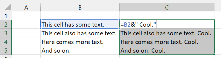
In this example, you have existing in cells B2 to B5. You want to add the word “Cool.” to it. So, the formula in cell C2 is:
=B2&" Cool."Please note that I have added a space before the word cool (on purpose…). The reason is that between the previous full stops and the word cool should have a space.
You can now copy the new cell (range C2 to C5). Paste it using paste special on top of the existing cells as values if you want to fully replace the original text cells.
Method 3: Try a workaround to insert text with the Find & Replace function
Admittedly, this method is a little bit trial and error. If it works depends on your existing cells. The main idea is to replace text from the original cells with new text.
Let’s go back to our original example. You again want to add the word “Cool.” to your existing cells:
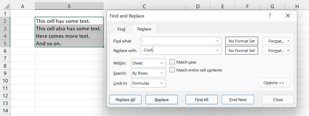
In this case, we are lucky that all existing cells end with a full stop. We can use this to replace it the following way:
- Select all original cells.
- Press Ctrl + H on the keyboard so that the Find and Replace window opens.
- As “Find what:”, enter “.”
- Because we still want to keep the full stop, we also use this in the “Replace with:” field: “. Cool.”
- Click on Replace All.
If the result is not as expected, you can simply undo the replace process (press Ctrl + Z on the keyboard).
Method 4: Bulk insert text with a VBA macro
If you feel comfortable to use a short VBA macro, you can copy and paste the following code into a new VBA module. Please refer to this article for help.
Replace the word ” Cool.” with your text to add at the end. Also, you can set a text to insert in the beginning. Then, place the cursor within these lines of code and press F5 on the keyboard.
Sub bulkInsertText()
    Dim textToInsertAtTheEnd As String, textToInsertAtTheBeginning As String

    'Replace "Cool" with your text to insert at the end
    textToInsertAtTheEnd = " Cool."
    textToInsertAtTheBeginning = ""

    For Each cell In Selection
        If cell.HasFormula = False Then
            cell.Value = textToInsertAtTheBeginning & cell.Value & textToInsertAtTheEnd
        End If
    Next

End Sub
Image by Gerd Altmann from Pixabay

Henrik Schiffner is a freelance business consultant and software developer. He lives and works in Hamburg, Germany. Besides being an Excel enthusiast he loves photography and sports.
I’ve been working with SQL and Excel Macros, but I don’t know how to add text to a cell.
I wish to add the text "01/01/13 00:00" to cell A1. I can’t just write it in the cell because the macro clears the contents of the sheet first and adds the information afterwards.
How do I do that in VBA?
![]()
asked Dec 16, 2013 at 13:43
![]()
2
Range("$A$1").Value = "'01/01/13 00:00" will do it.
Note the single quote; this will defeat automatic conversion to a number type. But is that what you really want? An alternative would be to format the cell to take a date-time value. Then drop the single quote from the string.
answered Dec 16, 2013 at 13:44
![]()
BathshebaBathsheba
231k33 gold badges359 silver badges477 bronze badges
3
You could do
[A1].Value = "'O1/01/13 00:00"
if you really mean to add it as text (note the apostrophe as the first character).
The [A1].Value is VBA shorthand for Range("A1").Value.
If you want to enter a date, you could instead do (edited order with thanks to @SiddharthRout):
[A1].NumberFormat = "mm/dd/yyyy hh:mm;@"
[A1].Value = DateValue("01/01/2013 00:00")
answered Dec 16, 2013 at 13:47
![]()
FlorisFloris
45.7k6 gold badges70 silver badges122 bronze badges
7
You need to use Range and Value functions.
Range would be the cell where you want the text you want
Value would be the text that you want in that Cell
Range("A1").Value="whatever text"
![]()
answered Mar 7, 2016 at 10:21
![]()
GarryGarry
611 silver badge1 bronze badge
You can also use the cell property.
Cells(1, 1).Value = "Hey, what's up?"
Make sure to use a . before Cells(1,1).Value as in .Cells(1,1).Value, if you are using it within With function. If you are selecting some sheet.
![]()
enamoria
8762 gold badges11 silver badges29 bronze badges
answered Dec 19, 2018 at 6:40
![]()