

Try it!
Use filters to temporarily hide some of the data in a table, so you can focus on the data you want to see.
Filter a range of data
-
Select any cell within the range.
-
Select Data > Filter.

-
Select the column header arrow
. -
Select Text Filters or Number Filters, and then select a comparison, like Between.
-
Enter the filter criteria and select OK.

 .
.

Filter data in a table
When you Create and format tables, filter controls are automatically added to the table headers.

-
Select the column header arrow
for the column you want to filter. -
Uncheck (Select All) and select the boxes you want to show.
-
Click OK.

The column header arrow  changes to a
  Filter icon. Select this icon to change or clear the filter.
Want more?
Filter data in a range or table
Filter data in a PivotTable
Need more help?
Want more options?
Explore subscription benefits, browse training courses, learn how to secure your device, and more.
Communities help you ask and answer questions, give feedback, and hear from experts with rich knowledge.
What is Filter in Excel?
The filter in excel helps display relevant data by eliminating the irrelevant entries temporarily from the view. The data is filtered as per the given criteria. The purpose of filtering is to focus on the crucial areas of a dataset. For example, the city-wise sales data of an organization can be filtered by the location. Hence, the user can view the sales of selected cities at a given time.
A filter is necessarily required when working with a huge database. Being a widely used tool, the filter converts a comprehensive view into an easy-to-understand one. To apply filters, the dataset must contain a header row which specifies the name of every column.
Table of contents
- What is Filter in Excel?
- How to Filter in Excel?
- Method 1: With Filter Option Under the Home tab
- Method 2: With Filter Option Under the Data tab
- Method 3: With the Shortcut key
- How to Add Filters in Excel?
- Example #1–“Number Filters” Option
- Example #2–“Search Box” Option
- Option while you Drop Down the Filter Function
- The Techniques of Filtering in Excel
- Frequently Asked Questions
- Recommended Articles
- How to Filter in Excel?
How to Filter in Excel?
You can download this Filter Column Excel Template here – Filter Column Excel Template
It is good to work with filters because they fit our needs the way we want to. In order to filter data, select the entries to be visible and deselect the rest of the items.
The three methods to add filters in excel are listed as follows:
- With filter option under the Home tab
- With filter option under the Data tab
- With the shortcut key
Let us consider a dataset to go through the three methods of adding filters.
The following table shows the invoices issued to the buyers of different cities. We want to filter the data using different methods.

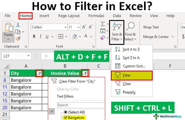
Method 1: With Filter Option Under the Home tab
In the Home tab, there is a “filter” option under the “sort and filter” drop-down of the “editing” section, as shown in the following image.
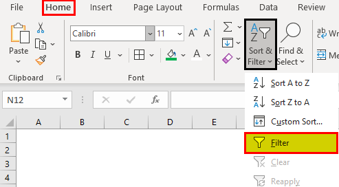
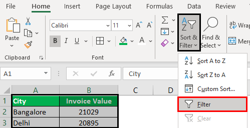
Step 1: Select the data and click “filter” under the “sort and filter” drop-down.
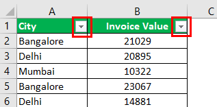
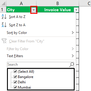
Step 2: The filters are added to the selected data range. The drop-down arrows, shown within the red boxes in the following image, are filters.
Step 3: Click the drop-down arrow of the column “city” to view the different names of the cities.
Step 4: To see the invoice values of “Delhi” only, select “Delhi” and uncheck all the remaining boxes.
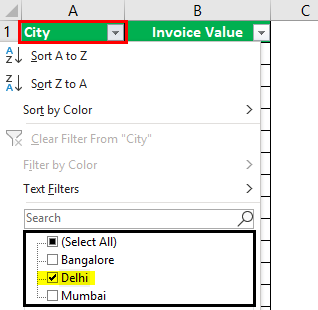
Step 5: The data for the city “Delhi” is filtered and displayed in the following image.

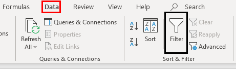
Method 2: With Filter Option Under the Data tab
In the Data tab, there is a “filter” option under the “sort and filter” section, as shown in the following image.
Method 3: With the Shortcut key
The keyboard shortcutsAn Excel shortcut is a technique of performing a manual task in a quicker way.read more are a good way to speed up the daily tasks. Select the data and add the filter using either of the following shortcuts:
- Press the keys “Shift+Ctrl+L” together.

- Press the keys “Alt+D+F+F” together.

Note: The preceding shortcuts for adding filtersUsing sorting and filtering, we can see the data category wise. With filtering data quickly you can easily navigate through menus or clicking through a mouse in less time.read more are toggle keys. Repetitive pressing helps to turn on and turn off the filters.
How to Add Filters in Excel?
We can filter numbers using advanced techniques. Let us consider some examples to understand the working of filters in Excel.
Example #1–“Number Filters” Option
Working on the data under the preceding heading (methods of filtering in Excel), we want to apply the following filters:
a. To filter column B (invoice value) for numbers greater than 10000
b. To filter column B for numbers greater than 10000 but less than 20000
Let us go through the two cases one by one.
a. Filter numbers greater than 10000
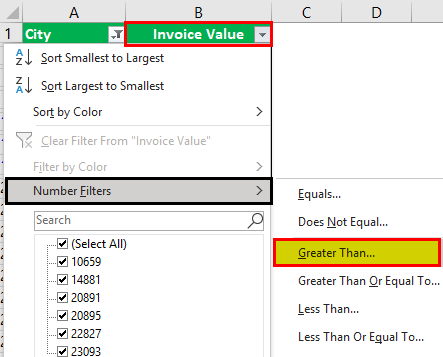
Step 1: Open the filter in column B (invoice value) by clicking on the filter symbol.
Step 2: In “number filters,” choose the “greater than” option, as shown in the following image.
Step 3: The “custom autofilter” box appears.
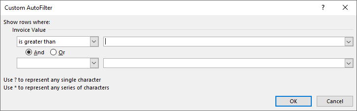
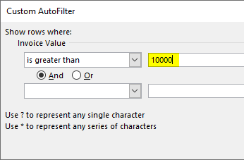
Step 4: Enter the number 10000 in the box to the right of “is greater than.”
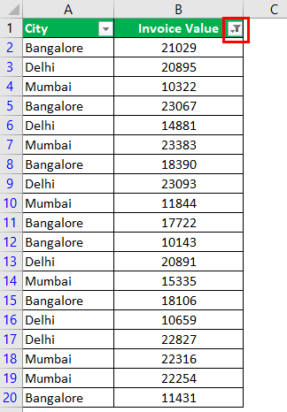
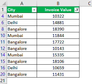
Step 5: The output displays the invoice values greater than 10000. The symbol within the red box is the filter icon. It indicates that the filter has been applied to column B.
b. Filter numbers greater than 10000 but less than 20000
Step 1: In “number filters,” choose the “greater than” option.
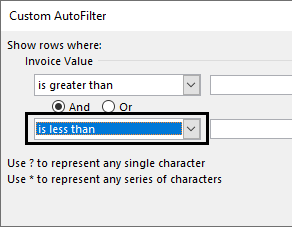
Step 2: In the “custom autofilter” box, select “is less than” in the second box to the left-hand side. This is shown in the following image.
Step 3: Enter the number 10000 in the box to the right of “is greater than.” Enter the number 20000 in the box to the right of “is less than.”
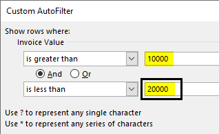
Step 4: The output displays the invoice values greater than 10000 but less than 20000.
Example #2–“Search Box” Option
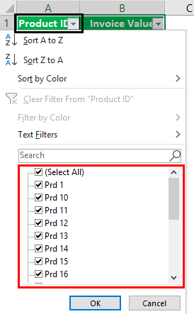
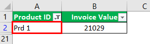
Working on the data under the preceding heading (methods of filtering in Excel), we have replaced the first column (city) with product IDs.
We want to filter the details of product ID “prd 1.”
The steps are listed as follows:
Step 1: Add filters to the columns “product ID” and “invoice value.”
Step 2: In the search boxA search box in Excel finds the needed data by typing into it, then filters the data and displays only that much info. When working with large datasheets, this simple tool may save a lot of time.read more, enter the value that is to be filtered. So, enter “prd 1.”
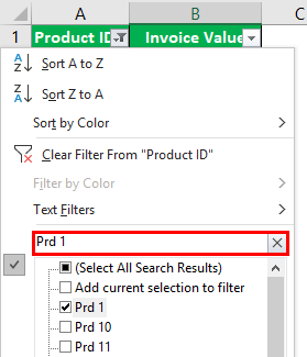
Step 3: The output displays only the filtered value from the list, as shown in the following image. Hence, we can see the invoice value of the product ID “prd 1.”
Option while you Drop Down the Filter Function
- Sort A to Z and Sort Z to A: If you wish to arrange your data ascending or descending order.
- Sort by Color: If you want to filter the data by color if a cell is filled by color.
- Text filter: When you want to filter a column with some exact text or number.
- Filter cells that begin with or end with an exact character or the text
- Filter cells that contain or do not contain a given character or word anywhere in the text.
- Filter cells that are exactly equal or not equal to a detailed character.
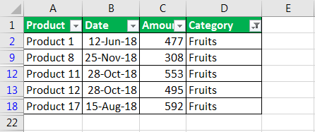
For example:
- Suppose you want to use the filter for a specific item. Click on to text filter and choose equals.
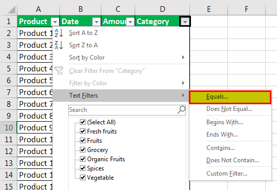
- It enables you the one dialogue, which includes a Custom Auto-Filter dialogue box.
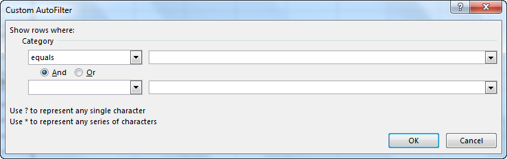
- Enter fruits under category and click Ok.
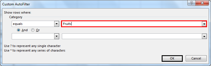
- Now you will get the data of fruits category only as shown below.
The Techniques of Filtering in Excel
The following techniques must be followed while filtering data:
- If the dataset is large, type the value to be filtered. This filters all the possible matches.
- If numerical data has to be filtered by specifying the greater than or the less than number, use the “number filters” option.
- If data has to be filtered by the color of specific rows, use the “filter by color” option.
Frequently Asked Questions
1. What are filters and how to add them in Excel?
Filtering is a technique which displays the required information and removes the unwanted data from the view. It helps the user focus on the relevant data at a given time.
The steps to add filters in Excel are listed as follows:
• Ensure that a header row appears on top of the data, specifying the column labels.
• Select the data on which filters are to be added.
• Add filters by any of the three given methods.
o Click the “filter” option under the “sort and filter” (editing section) drop-down of the Home tab.
o Click the “filter” option under the “sort and filter” section of the Data tab.
o Press the keys “Shift+Ctrl+L” or “Alt+D+F+F.”
Note: As soon as the filters are added, a drop-down arrow appears on the particular column header.
2. How to apply filters to one or more columns?
The steps to apply filters to one or more columns are listed as follows:
• Click the drop-down arrow of the column to be filtered.
• Uncheck the “select all” option which helps deselect all data.
• Select the boxes to be displayed.
• Click “Ok.”
The drop-down arrow changes to the filter icon as soon as a filter is applied. When filters are applied to multiple columns, the filter icon appears on each one of them. Hovering over the filter icon shows the filters that have been applied.
Note: The drop-down arrow on a column header indicates a filter is added. The filter icon indicates a filter has been applied.
3. How to use filters in Excel?
The filters can be applied to numbers, text values, and dates. These cases are discussed as follows:
Filter numbers
• Click on the “number filters.”
• Select any of the options like “equals,” “does not equals,” “greater than,” “less than,” “between,” “above average,” and so on.
• Specify the required fields in the dialog box that appears. This box may or may not be displayed.
For instance, in “equals,” enter the number against which the values should be compared. The filtered results show the matching numerical values.
Filter text and date values
• To filter text and date values, select “text filters” and “date filters” from the respective drop-down arrows.
• The “text filters” allow filtering text strings which contain specific characters or words. The “date filters” allow filtering dates for a particular year, month, week, and so on.
Note: The “plus” and the “minus” sign of the date filters are used for expanding and collapsing the various levels respectively.
Recommended Articles
This has been a guide to Filter in Excel. Here we discuss how to use/add filters in excel along with step by step examples and a downloadable template. You may learn more about Excel from the following articles –
- VBA FilterThe VBA Filter tool is used to sort out or fetch the desired data. However, this function accepts optional arguments, and the only required argument is an expression that covers the range, such as worksheets(«Sheet1»). Range(“A1”).read more
- How to Filter Pivot Table?By right-clicking on the pivot table, we can access the pivot table filter option. Another approach is to use the filter options available in the pivot table fields.read more
- Advanced Filter in ExcelThe advanced filter is different from the auto filter in Excel. This feature is not like a button that one can use with a single click of the mouse. To use an advanced filter, we have to define criteria for the auto filter and then click on the “Data” tab. Then, in the advanced section for the advanced filter, we will fill our criteria for the data.read more
- Types of Filters in Power BIThe filter function in Power BI is more commonly used to read data or reports based on multiple criteria. Visual level filters, page-level filters, report-level filters, drill-through filters, and so on are all available filters in Power Bi.read more
#Руководства
- 5 авг 2022
-
0
Как из сотен строк отобразить только необходимые? Как отфильтровать таблицу сразу по нескольким условиям и столбцам? Разбираемся на примерах.
Иллюстрация: Meery Mary для Skillbox Media

Рассказывает просто о сложных вещах из мира бизнеса и управления. До редактуры — пять лет в банке и три — в оценке имущества. Разбирается в Excel, финансах и корпоративной жизни.
Фильтры в Excel — инструмент, с помощью которого из большого объёма информации выбирают и показывают только нужную в данный момент. После фильтрации в таблице отображаются данные, которые соответствуют условиям пользователя. Данные, которые им не соответствуют, скрыты.
В статье разберёмся:
- как установить фильтр по одному критерию;
- как установить несколько фильтров одновременно и отфильтровать таблицу по заданному условию;
- для чего нужен расширенный фильтр и как им пользоваться;
- как очистить фильтры.
Фильтрация данных хорошо знакома пользователям интернет-магазинов. В них не обязательно листать весь ассортимент, чтобы найти нужный товар. Можно заполнить критерии фильтра, и платформа скроет неподходящие позиции.
Фильтры в Excel работают по тому же принципу. Пользователь выбирает параметры данных, которые ему нужно отобразить, — и Excel убирает из таблицы всё лишнее.
Разберёмся, как это сделать.
Для примера воспользуемся отчётностью небольшого автосалона. В таблице собрана информация о продажах: характеристики авто, цены, даты продажи и ответственные менеджеры.
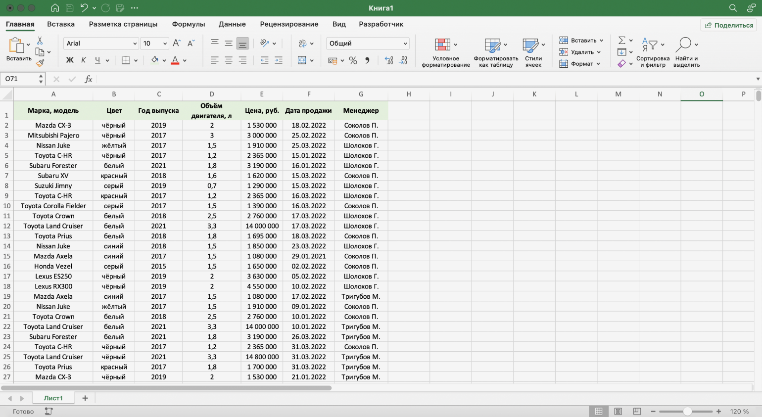
Скриншот: Excel / Skillbox Media
Допустим, нужно показать продажи только одного менеджера — Соколова П. Воспользуемся фильтрацией.
Шаг 1. Выделяем ячейку внутри таблицы — не обязательно ячейку столбца «Менеджер», любую.
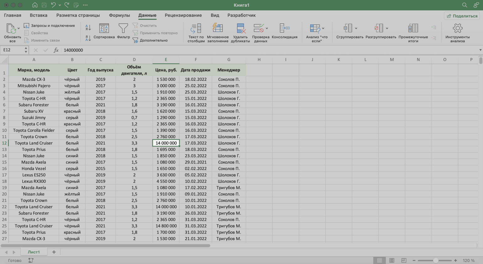
Скриншот: Excel / Skillbox Media
Шаг 2. На вкладке «Главная» нажимаем кнопку «Сортировка и фильтр».
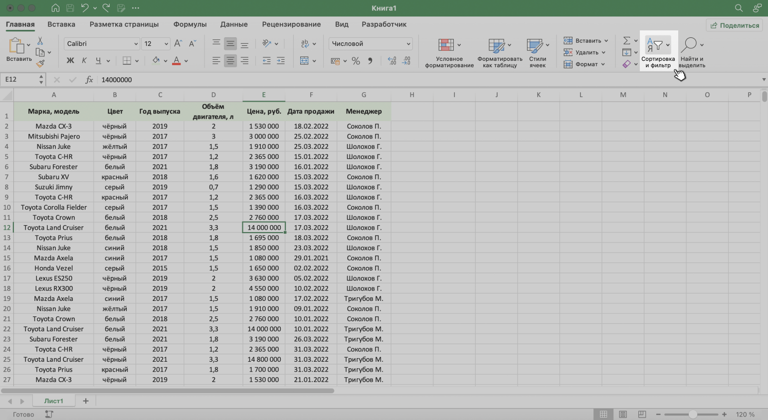
Скриншот: Excel / Skillbox Media
Шаг 3. В появившемся меню выбираем пункт «Фильтр».
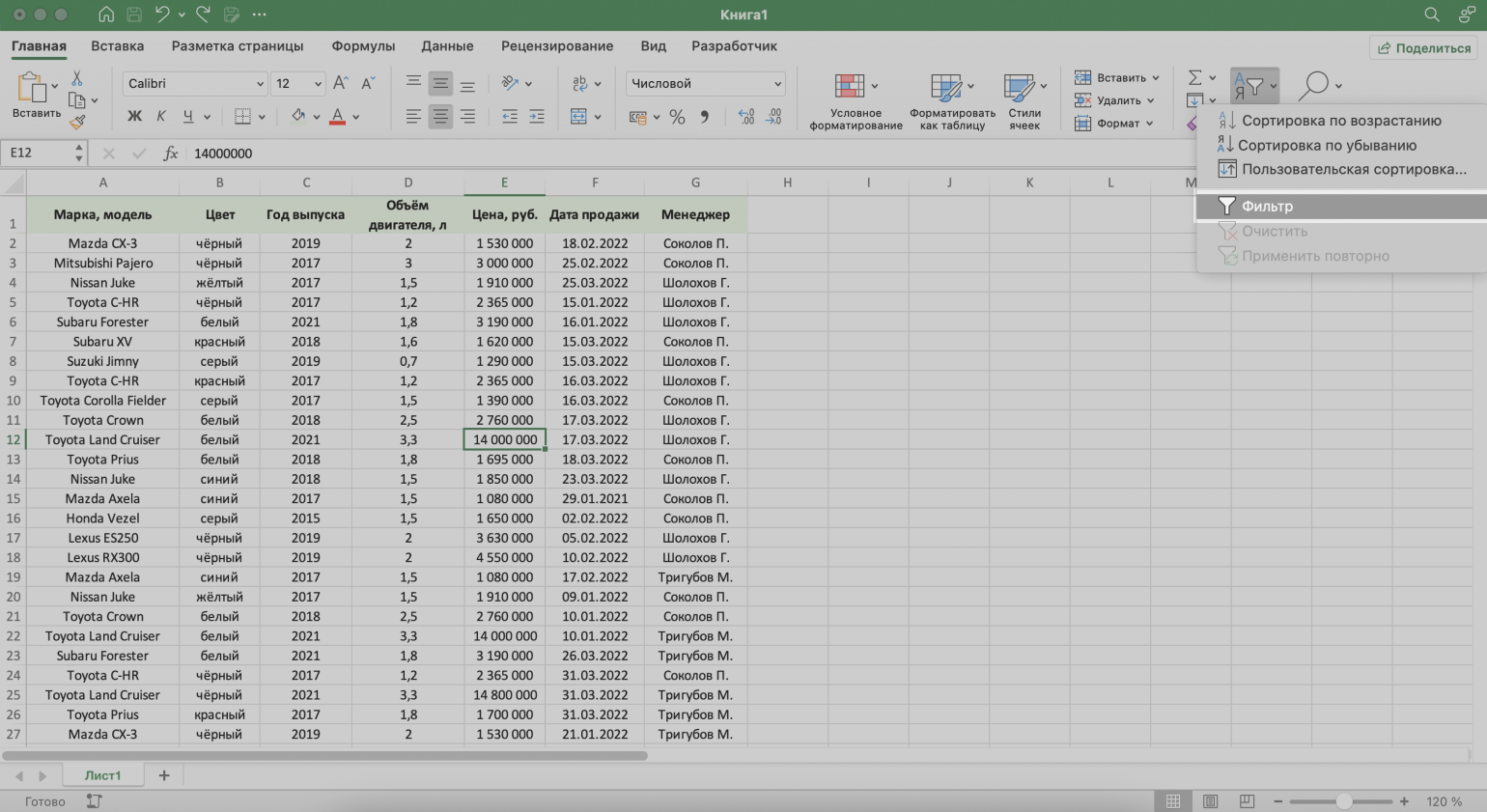
Скриншот: Excel / Skillbox Media
То же самое можно сделать через кнопку «Фильтр» на вкладке «Данные».
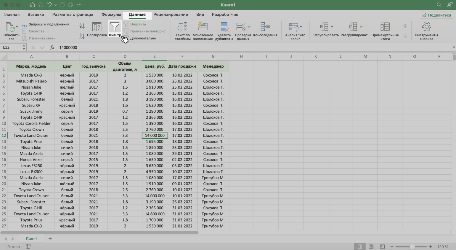
Скриншот: Excel / Skillbox Media
Шаг 4. В каждой ячейке шапки таблицы появились кнопки со стрелками — нажимаем на кнопку столбца, который нужно отфильтровать. В нашем случае это столбец «Менеджер».
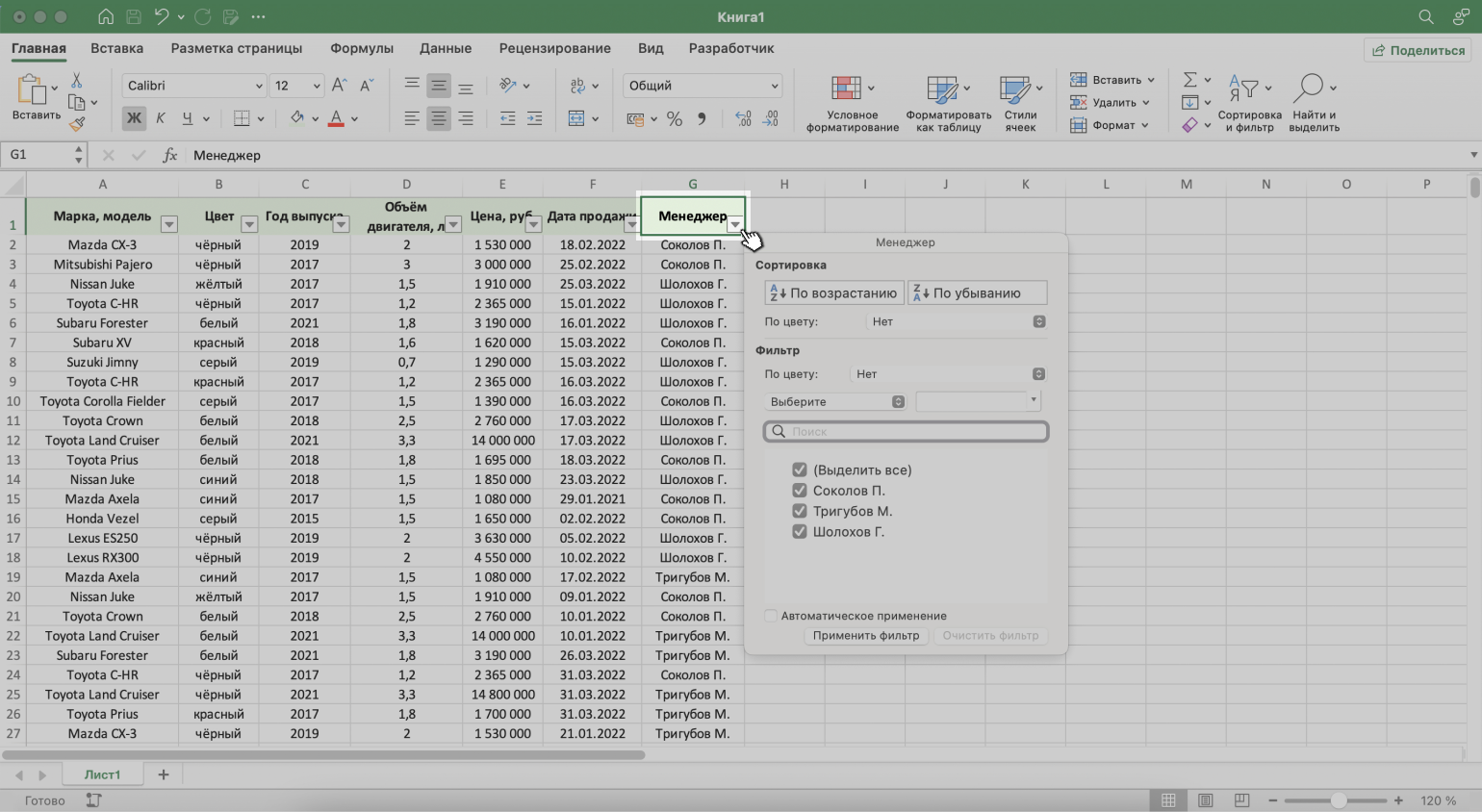
Скриншот: Excel / Skillbox Media
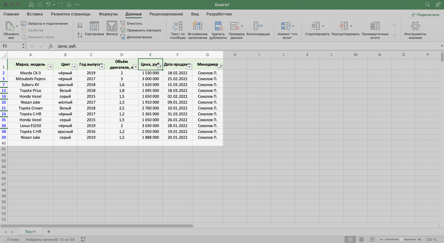
Шаг 5. В появившемся меню флажком выбираем данные, которые нужно оставить в таблице, — в нашем случае данные менеджера Соколова П., — и нажимаем кнопку «Применить фильтр».
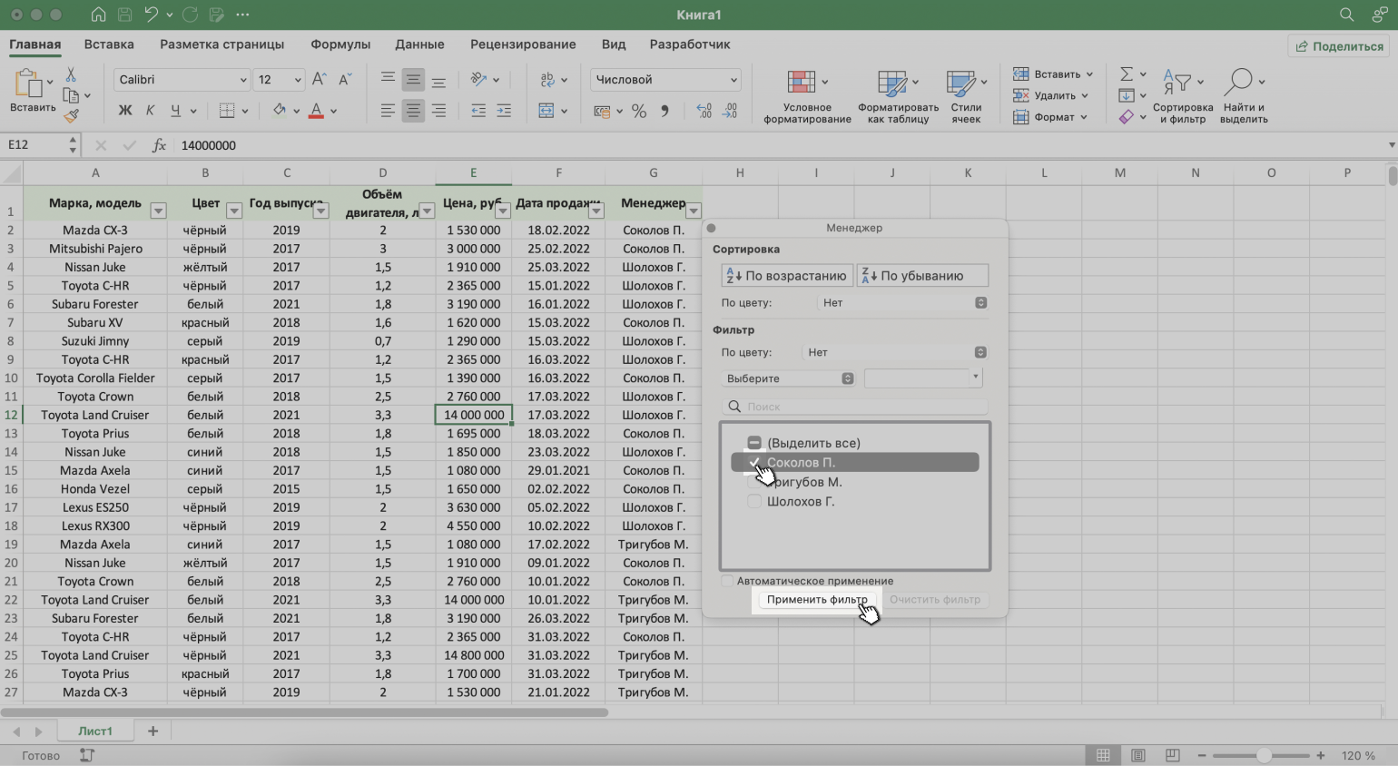
Скриншот: Excel / Skillbox Media
Готово — таблица показывает данные о продажах только одного менеджера. На кнопке со стрелкой появился дополнительный значок. Он означает, что в этом столбце настроена фильтрация.
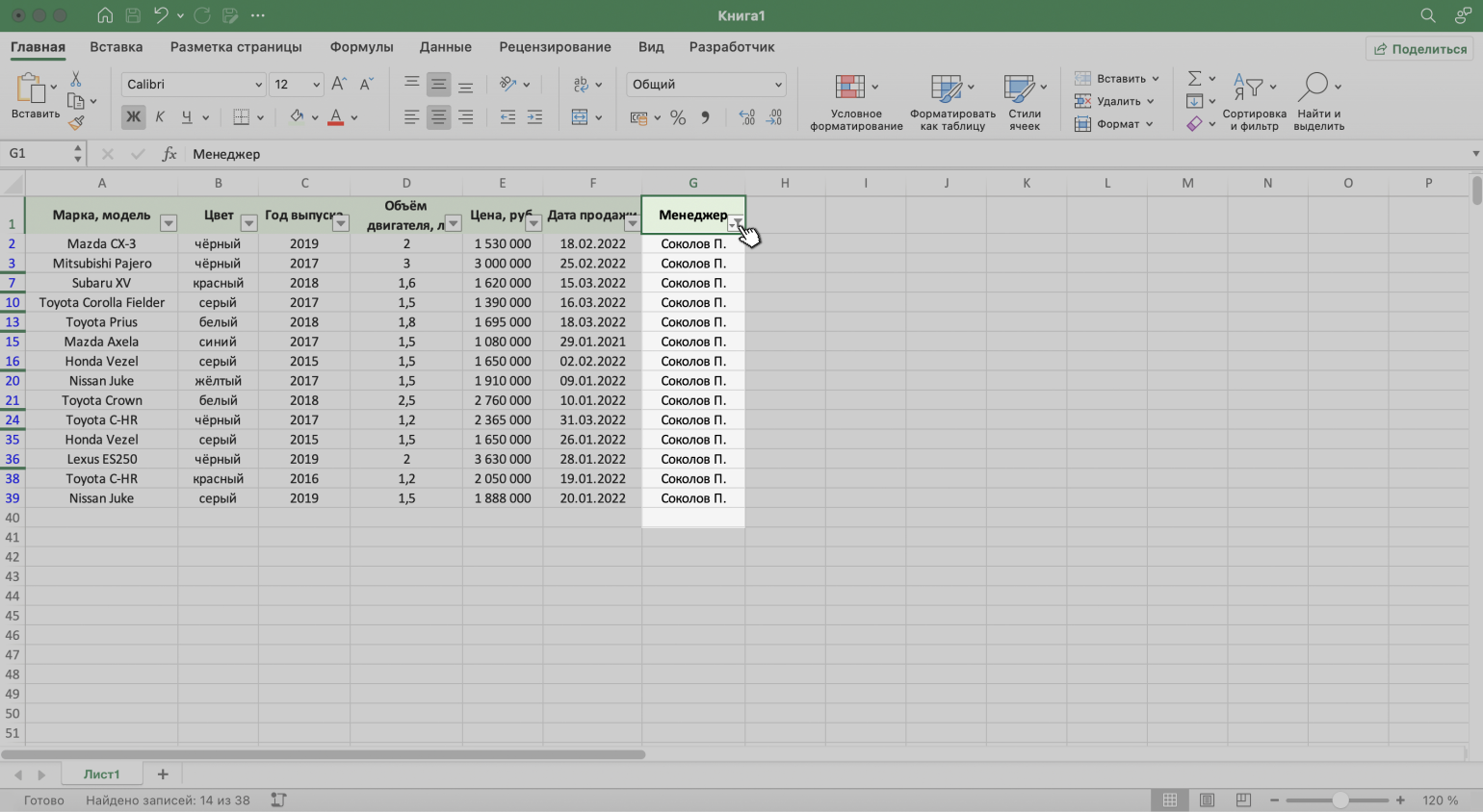
Скриншот: Excel / Skillbox Media
Чтобы ещё уменьшить количество отображаемых в таблице данных, можно применять несколько фильтров одновременно. При этом как фильтр можно задавать не только точное значение ячеек, но и условие, которому отфильтрованные ячейки должны соответствовать.
Разберём на примере.
Выше мы уже отфильтровали таблицу по одному параметру — оставили в ней продажи только менеджера Соколова П. Добавим второй параметр — среди продаж Соколова П. покажем автомобили дороже 1,5 млн рублей.
Шаг 1. Открываем меню фильтра для столбца «Цена, руб.» и нажимаем на параметр «Выберите».
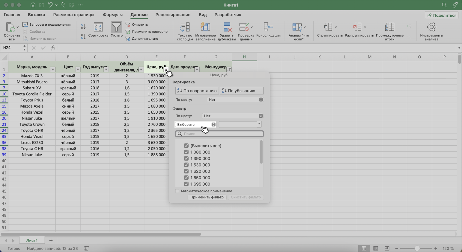
Скриншот: Excel / Skillbox Media
Шаг 2. Выбираем критерий, которому должны соответствовать отфильтрованные ячейки.
В нашем случае нужно показать автомобили дороже 1,5 млн рублей — выбираем критерий «Больше».
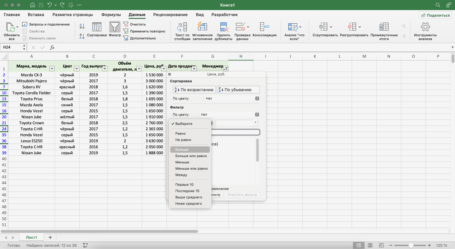
Скриншот: Excel / Skillbox Media
Шаг 3. Дополняем условие фильтрации — в нашем случае «Больше 1500000» — и нажимаем «Применить фильтр».
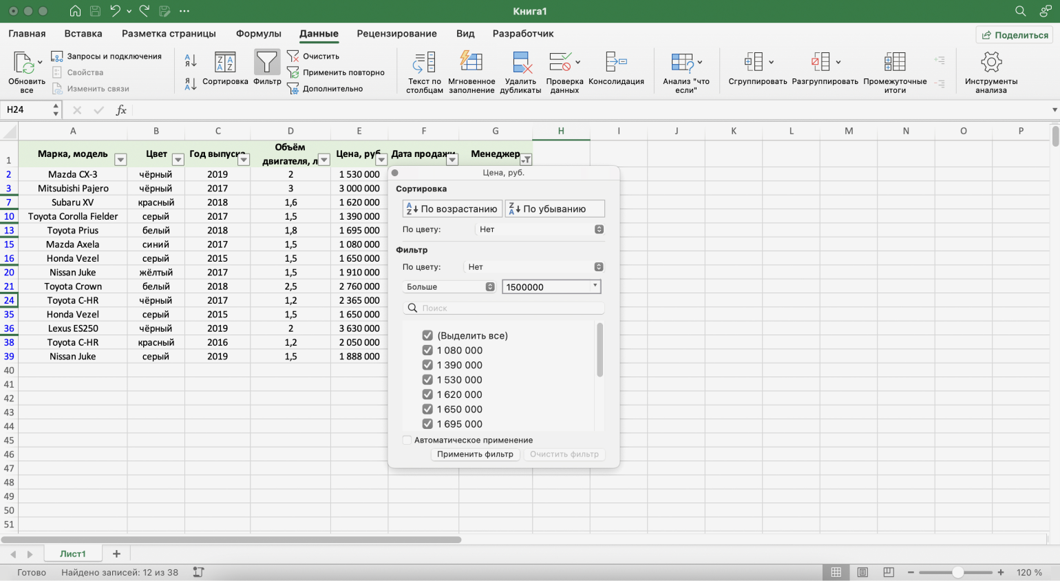
Скриншот: Excel / Skillbox Media
Готово — фильтрация сработала по двум параметрам. Теперь таблица показывает только те проданные менеджером авто, цена которых была выше 1,5 млн рублей.
Скриншот: Excel / Skillbox Media
Расширенный фильтр позволяет фильтровать таблицу по сложным критериям сразу в нескольких столбцах.
Это можно сделать способом, который мы описали выше: поочерёдно установить несколько стандартных фильтров или фильтров с условиями пользователя. Но в случае с объёмными таблицами этот способ может быть неудобным и трудозатратным. Для экономии времени применяют расширенный фильтр.
Принцип работы расширенного фильтра следующий:
- Копируют шапку исходной таблицы и создают отдельную таблицу для условий фильтрации.
- Вводят условия.
- Запускают фильтрацию.
Разберём на примере. Отфильтруем отчётность автосалона по трём критериям:
- менеджер — Шолохов Г.;
- год выпуска автомобиля — 2019-й или раньше;
- цена — до 2 млн рублей.
Шаг 1. Создаём таблицу для условий фильтрации — для этого копируем шапку исходной таблицы и вставляем её выше.
Важное условие — между таблицей с условиями и исходной таблицей обязательно должна быть пустая строка.
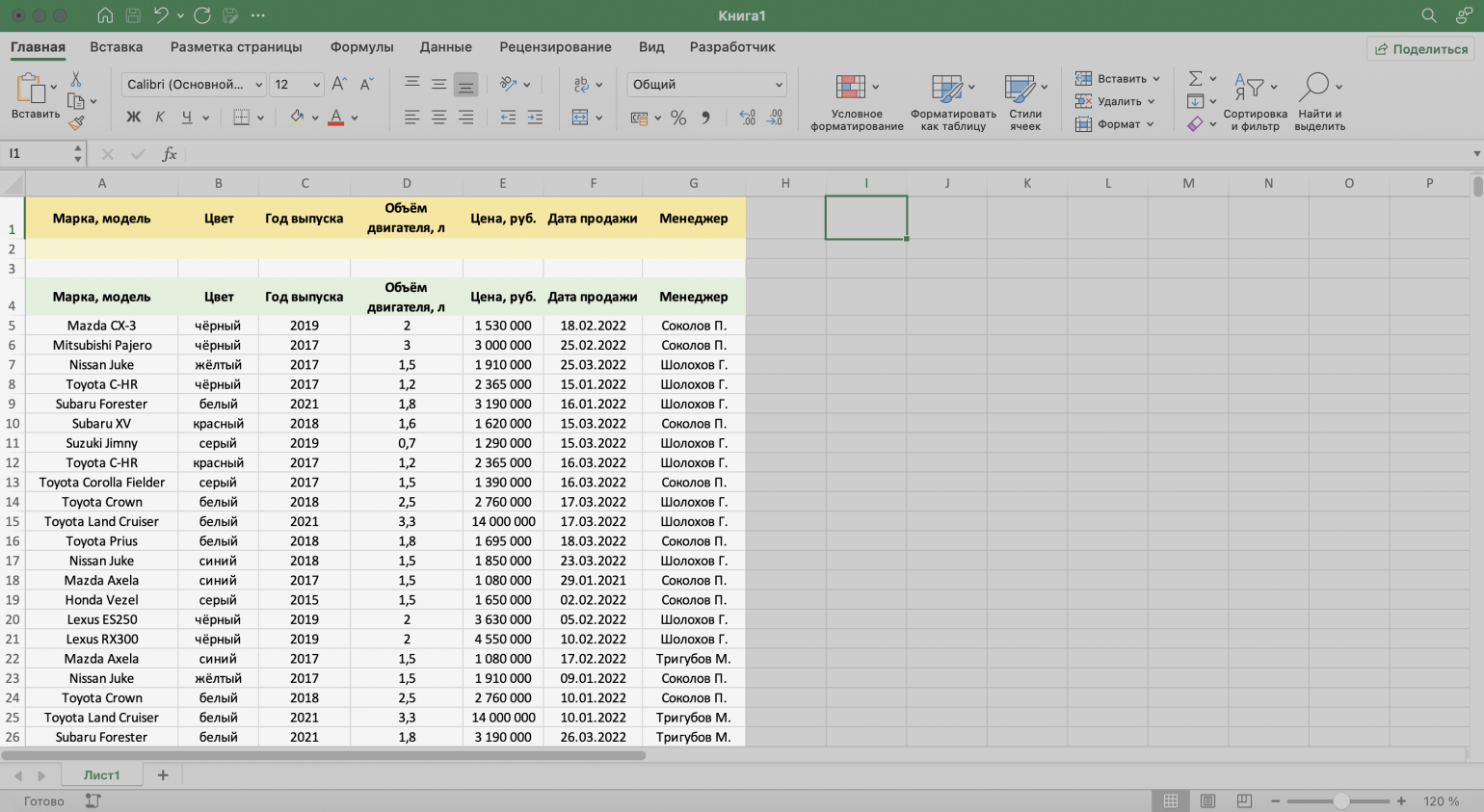
Скриншот: Excel / Skillbox Media
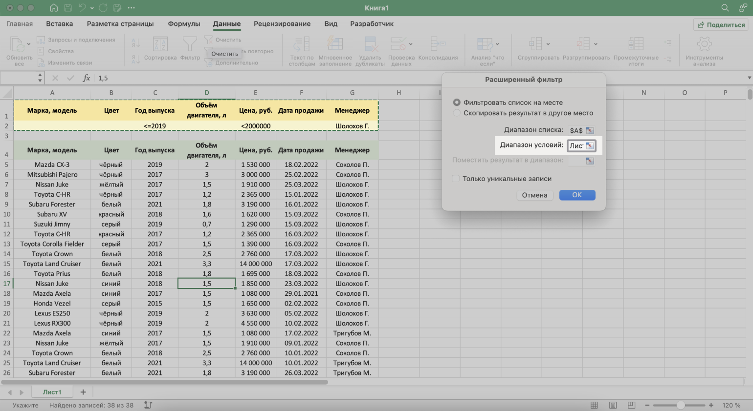
Шаг 2. В созданной таблице вводим критерии фильтрации:
- «Год выпуска» → <=2019.
- «Цена, руб.» → <2000000.
- «Менеджер» → Шолохов Г.
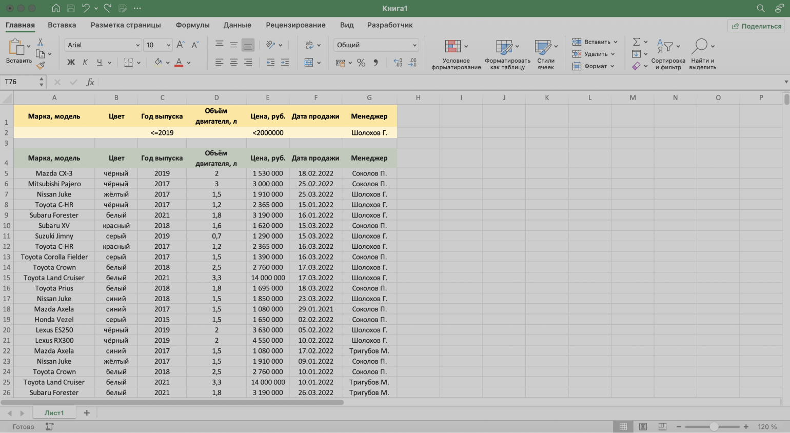
Скриншот: Excel / Skillbox Media
Шаг 3. Выделяем любую ячейку исходной таблицы и на вкладке «Данные» нажимаем кнопку «Дополнительно».
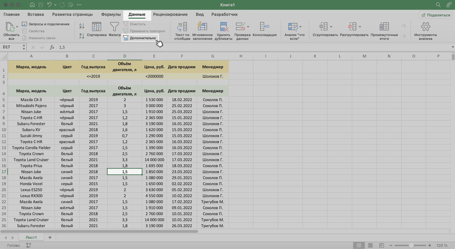
Скриншот: Excel / Skillbox Media
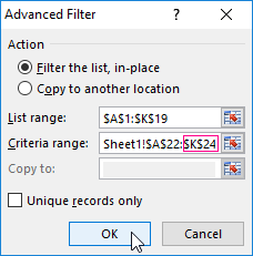
Шаг 4. В появившемся окне заполняем параметры расширенного фильтра:
- Выбираем, где отобразятся результаты фильтрации: в исходной таблице или в другом месте. В нашем случае выберем первый вариант — «Фильтровать список на месте».
- Диапазон списка — диапазон таблицы, для которой нужно применить фильтр. Он заполнен автоматически, для этого мы выделяли ячейку исходной таблицы перед тем, как вызвать меню.
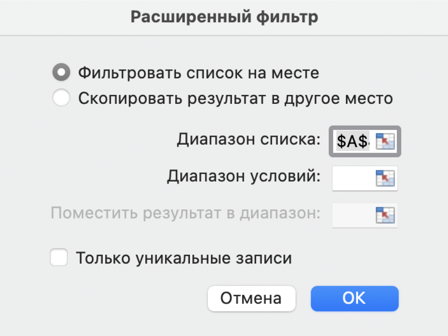
Скриншот: Excel / Skillbox Media
- Диапазон условий — диапазон таблицы с условиями фильтрации. Ставим курсор в пустое окно параметра и выделяем диапазон: шапку таблицы и строку с критериями. Данные диапазона автоматически появляются в окне параметров расширенного фильтра.
Скриншот: Excel / Skillbox Media
Шаг 5. Нажимаем «ОК» в меню расширенного фильтра.
Готово — исходная таблица отфильтрована по трём заданным параметрам.
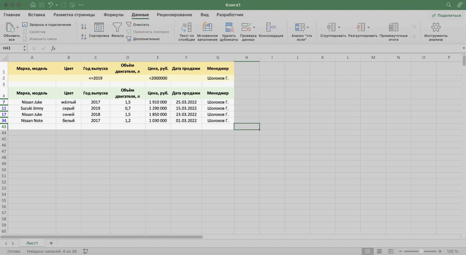
Скриншот: Excel / Skillbox Media
Отменить фильтрацию можно тремя способами:
1. Вызвать меню отфильтрованного столбца и нажать на кнопку «Очистить фильтр».
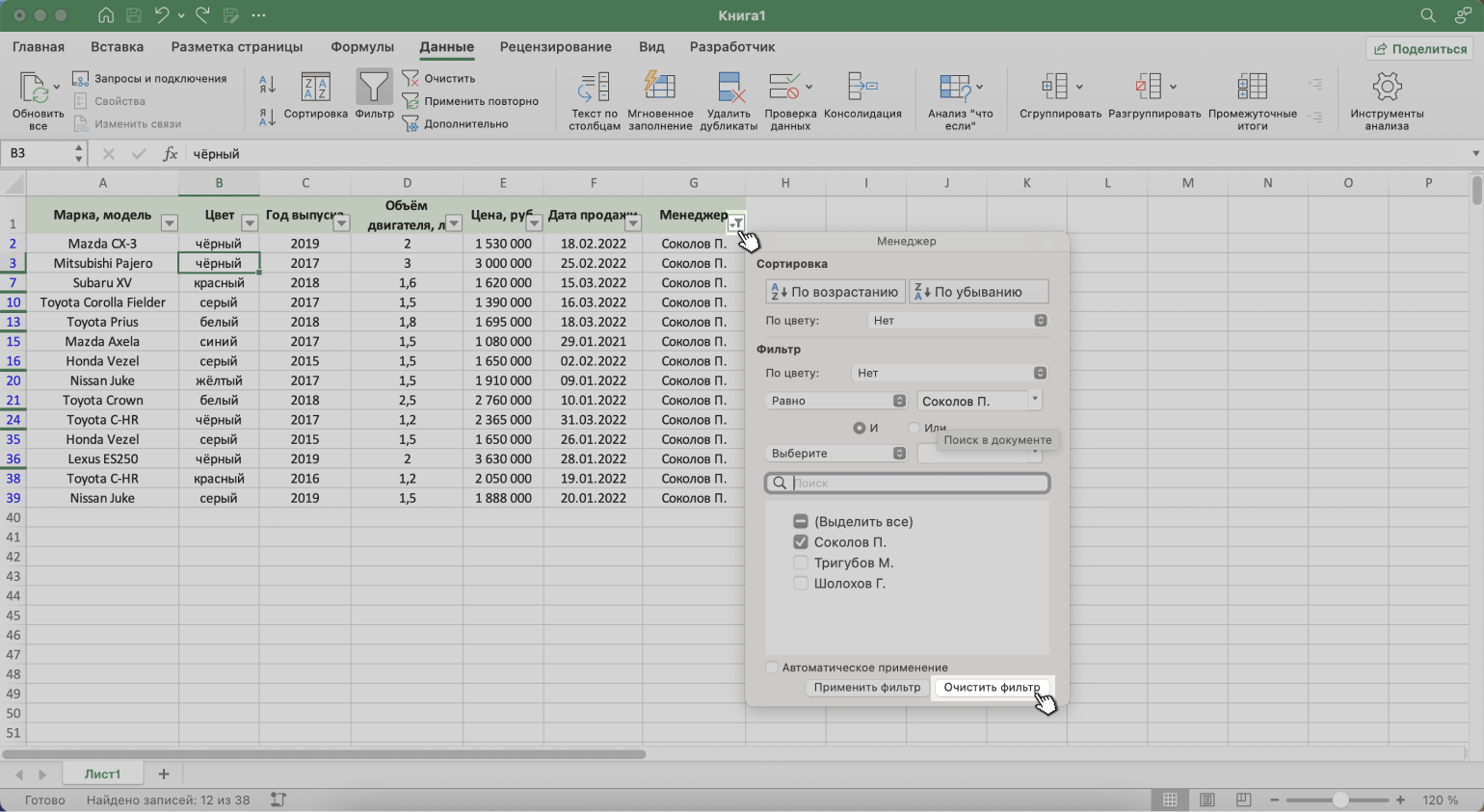
Скриншот: Excel / Skillbox Media
2. Нажать на кнопку «Сортировка и фильтр» на вкладке «Главная». Затем — либо снять галочку напротив пункта «Фильтр», либо нажать «Очистить фильтр».
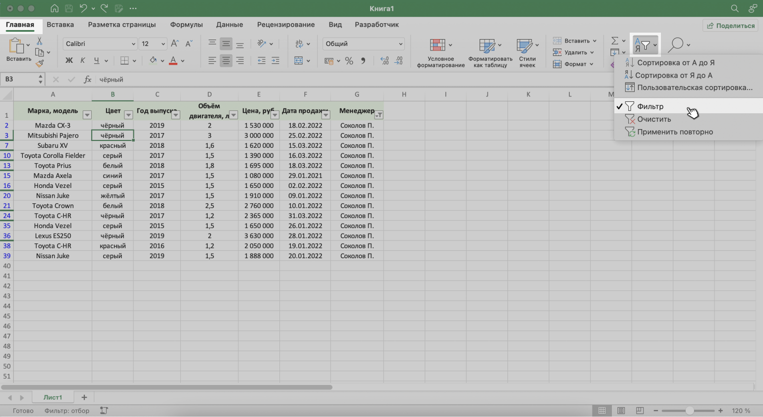
Скриншот: Excel / Skillbox Media
3. Нажать на кнопку «Очистить» на вкладке «Данные».
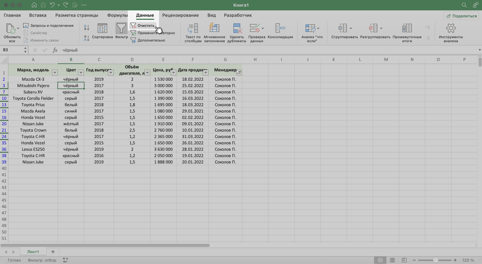
Скриншот: Excel / Skillbox Media

Научитесь: Excel + Google Таблицы с нуля до PRO
Узнать больше
Advanced filter in Excel provides more opportunities for managing on data management spreadsheets. It is more complex in settings, but much more effective in action.
Using a standard filter, a Microsoft Excel user can solve not all of the tasks that are set. There is no visual display of the applied filtering conditions. It is not possible to apply more than two selection criteria. You can not filter the duplicate values to leave only unique records. And the criteria themselves are schematic and simple. The functionality of the extended filter is much richer. Let’s take a closer look at its possibilities.
How to make the advanced filter in Excel?
The advanced filter allows you to analysis data on an unlimited set of conditions. With this tool, the user can:
- to specify more than two selection criteria;
- to copy the result of filtering to another sheet;
- to set the condition of any complexity with the helping of formulas;
- to extract the unique values.
The algorithm for applying the extended filter is simple.
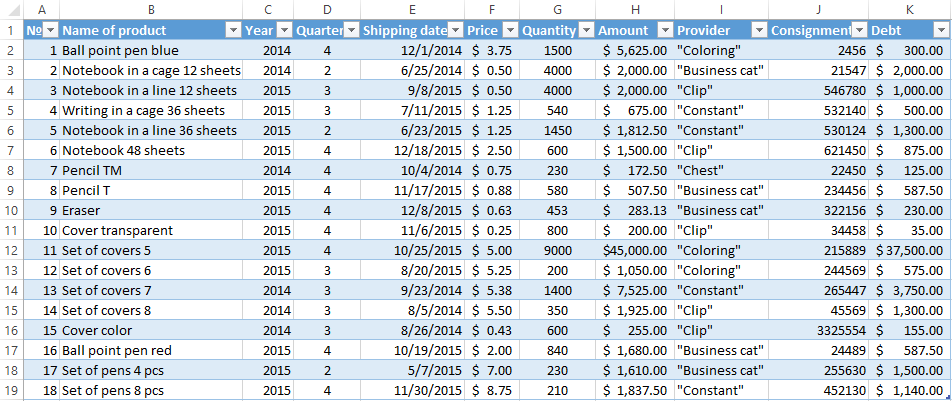
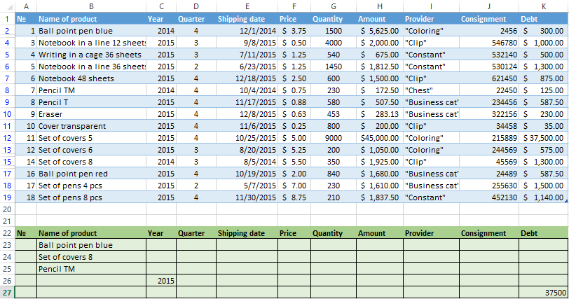
- To make the table with the original data or to open an existing one. Like so:
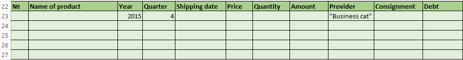
- To create the condition table. The features: the header line is the same with the «cap» of the filtered table. To avoid errors, need to copy the header line in the source table and paste it on the same sheet (side, top, underarm) or on another sheet. We enter the selection criteria into the condition table.
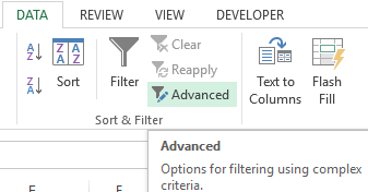
- Go to the «DATA» tab — «Sort and filter» — «Advanced». If the filtered information should be displayed on another sheet (NOT where the source table is), then you need to run the extended filter from another sheet.
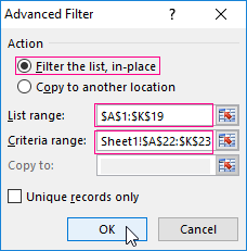
- In the «Advanced Filter» window that opens, to select the method of processing information (on the same sheet or on the other one), set the initial range (the table 1, example) and the range of conditions (the table 2, conditions). The header lines must be included in the ranges.
- To close the «Advanced Filter» window, click OK. We see the result.

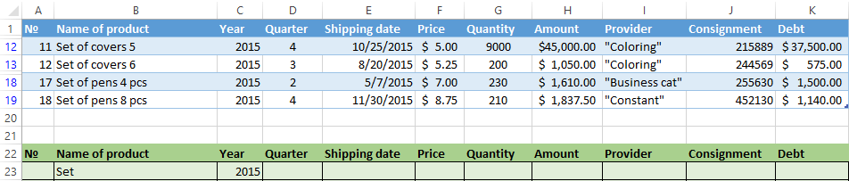
The top table is the result of the filtering. The lower nameplate with the conditions is given for clarity near.
How to use the advanced filter in Excel?
To cancel the action of the advanced filter, we place the cursor anywhere in the table and press Ctrl + Shift + L or «DATA» — «Sort and Filter» — «Clear».
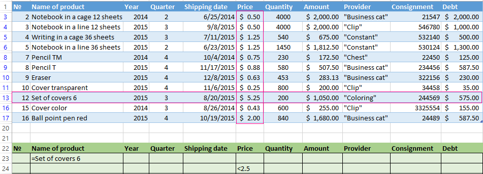
We will find using the «Advanced Filter» tool information on the values that contain the word «Set».
In the table of conditions we bring in the criteria. For example, these are:

The program in this case will search for all information on the goods, in the title of which there is the word «Set».
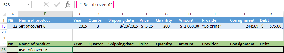
To search for the exact value, you can use the «=» sign. We enter the following criteria in the condition table:

Excel sees the «=» as a signal: the user will set the formula now. In order for the program to work correctly, the following should be written in the formula line: =»=Set of covers 6″.
After using the «Advanced Filter»:
We filter the source table by the condition «OR» for different columns now. The operator «OR» is also in the tool «AutoFilter». But there it can be used within the single column.
In the condition label we introduce the selection criteria: =»=Set of covers 6″. (In the column «Name of product») and = «<2.5$» (in the column «Price»). That is, the program must select those values that contain the EXACTLY information about the good «Set of covers 6 ». OR to the information about the goods, which price is <2.5.

Please note: the criteria must be written under the corresponding headings in the DIFFERENT lines.
The result of selection:
The advanced filter allows you to use as a criterion of a formula. Let’s consider the example.

Selection of the line with the maximum indebtedness: =MAX(Table1[Debt]).
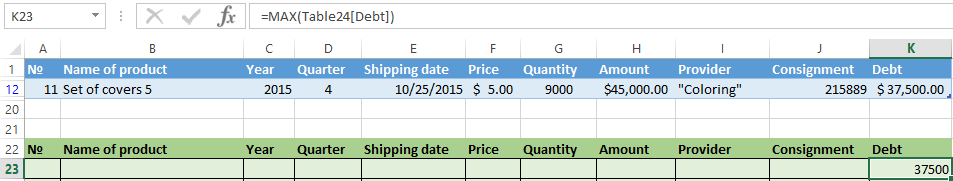
So we get the results as after running several filters on the one Excel sheet.
How to make few filters in Excel?
Let’s create the filter by several values. To do this, we enter in the table of conditions several criteria for selecting data:
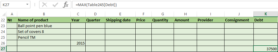
Apply the tool «Advanced Filter»:
Now from the table with the selected data we will extract new information, which was selected according to other criteria. There are only shipping date for autumn 2015 (from September to November). Example:
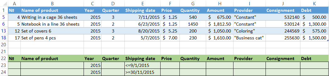
We introduce a new criterion in the condition table and apply the filtering tool. The initial range — is the table with data selected according to the previous criterion. This is how the filter is performed across on several columns.
To use few filters, you can create several condition tables on the new sheets. The method of implementation depends from the task which was set by user.
How to make the filter in Excel by lines?
By standard methods — you may not do it by any ways. Microsoft Excel selects data only in columns. Therefore, we need to look for other solutions.
Here are some examples of string criteria for the extended filter in Excel:
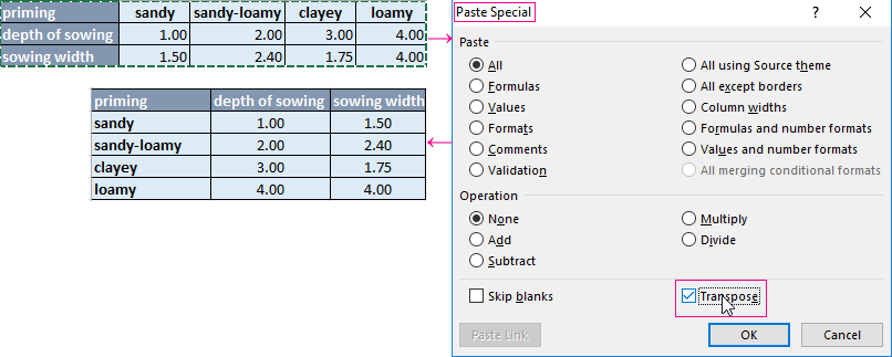
- Convert to the table. For example, from three rows make a list of three columns and apply the filtering to the transformed version.
- Use formulas to display exactly the data in the string that are needed. For example, make some indicator drop-down list. And in the next cell, enter the formula using the IF function. When a certain value is selected from the drop-down list, its parameter appears next to it.
To give an example of how the filter works by rows in Excel, we are creating the label:
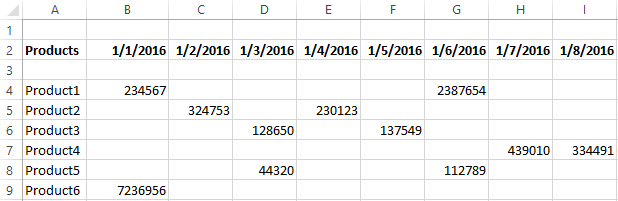
For the list of products, we create the drop-down list:
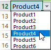
If necessary, learn how to create a drop-down list in Excel.
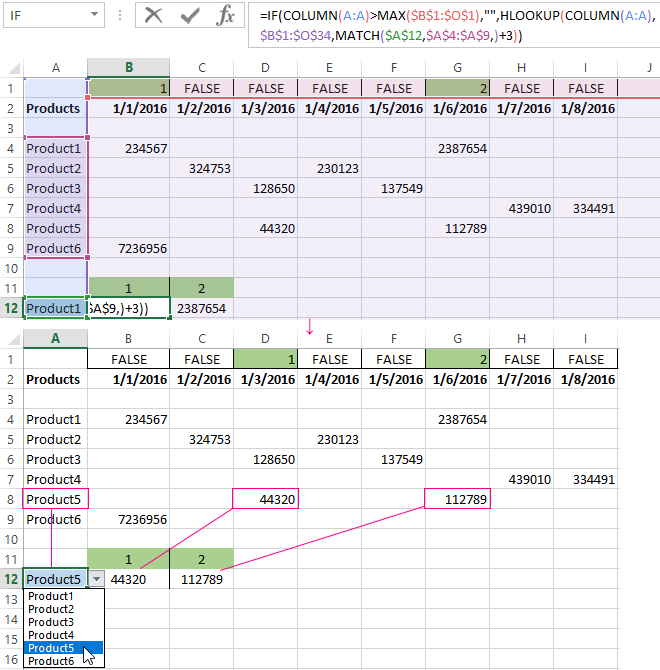
Above the table with the original data, we insert an empty line. In the cells, we introduce the formula that will show which columns the information is taken from.
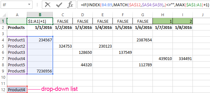
Next to the drop-down list box, we enter the following formula:
Its task is select from the table those values, that correspond to a certain good.
Download examples of advanced filtering
Thus, using the tool «Drop-down list» and built-in functions Excel selects data in rows according to a certain criterion.
Фильтры в таблице excel — это инструменты, которые способны отсеивать лишнюю информацию из таблицы и вычленять из нее только необходимую, соответствующую критериям. Программа позволяет устанавливать как простые условия поиска по одному параметру, так и сложные, по нескольким переменным.
Как поставить
Excel — мощная программа из пакета Microsoft, созданная для работы с таблицами. В ней удобно вести большой учет множества данных. И регулярно у пользователей возникает потребность быстро находить в файлах с тысячами данных те, которые отвечают определенному параметру. Для этого придется поставить фильтр в эксель-таблице.
Для начала работы необходимо выбрать одну, любую, ячейку внутри таблицы, открыть вкладку «Данные».

Затем нажать кнопку «Фильтр».

В заголовках столбцов появятся значки неиспользуемого отсева. Это означает, что осталось только установить нужные параметры, чтобы отсечь необходимую информацию.
В таблице
Пошаговая инструкция: как поставить фильтр в эксель-таблице.
1. Нажать на значок в заголовке столбца.

Перед пользователем появится выпадающее окошко с перечислением всех значений в этом столбце.

2. Убрать лишние галочки, стоящие у параметров, которые пользователя не интересуют. Галочки останутся только у тех параметров, по которым необходимо провести поиск. После чего нажать «Ок».

3. Просмотреть результат — останутся только строки, соответствующие заданному параметру.

В диапазоне
Отсев в диапазоне применяется, когда необходимо отсечь информацию не по одному значению, а по определенному спектру. Он бывает числовым или текстовым, в зависимости от информации, которую содержит необходимый столбец.
Например, в рассматриваемом файле столбцы В и С имеют числовой отсев.

Остальные — текстовый.

Чтобы установить диапазонный поиск, необходимо нажать значок в заголовке столбца, выбрать строку с наименованием отсева и необходимый способ установления диапазона, установить его и применить.
Например, в случае с числовым поиском этот порядок действий выглядит так:
1. Выбираем вид отсева.

2. Выбираем необходимый способ формирования диапазона, например, «больше» означает, что в результате появятся все значения, превышающие цифру, которую пользователь введет.

3. Ввести цифру, которая и станет границей для отсева, — выведены будут все значения больше нее.

4. Нажать «Ок» и оценить результат. В выбранном столбце останутся только значения, превышающие установленную границу.

Как задать несколько параметров
После того как информация отфильтрована по параметрам одного из столбцов, пользователь вправе продолжить отфильтровывать ее по остальным столбцам. Значений для отсева уже меньше, но результат станет более детальным.
Например, мы уже отфильтровали таблицу по условию «Страна» и оставили только товары российского происхождения.

Теперь необходимо дополнительно отделить товары стоимостью 100 рублей, для этого применяем отсев в разделе «Цена».

Нажимаем «Ок» и получаем только товары стоимостью 100 рублей, произведенные в России.

Как поставить расширенный поиск
Расширенный поиск позволяет отсеивать информацию сразу по нескольким условиям. Работая с ним, перед тем как поставить фильтр в таблице excel, необходимо подготовить саму таблицу — создать над ней поле из нескольких свободных строк и скопировать заголовки.

Затем в свободной строке под скопированными заголовками задать необходимые условия поиска. Например, необходимо найти товары, произведенные в России, проданные менеджером Ивановым, стоимостью менее 300 рублей.

После того как параметры корректно введены, необходимо снова открыть вкладку «Данные» и выбрать функцию «Дополнительно».

Перед пользователем появится окно, в котором ему предстоит заполнить две строки:
- «Исходный диапазон» — это диапазон таблицы, информация которой подлежит фильтрации, то есть исходной таблицы. Его эксель введет автоматически;
- «Диапазон условий» — это ячейки, из которых программа возьмет значения для отсева, — вторая таблица, которую мы создали сверху. Чтобы значения появились в строке окна, необходимо просто захватить две ее строки: с наименованием раздела и введенными значениями.

После того как оба диапазона сформированы, нажмите «Ок» и оцените результат.

Как удостовериться, поставлен ли фильтр
Чтобы узнать, установлен поиск данных или нет, необходимо взглянуть на строку с наименованием параметров — это первая строка. Если он есть, в каждой ячейке строки обнаружится небольшой значок.

Значком «1» обозначается столбец, в котором поиск установлен, но не применяется. Значком «2» обозначен уже примененный поиск.
Удаление
Эксель позволяет снимать фильтры по отдельности — с каждого раздела, к которому они были применены, или со всего файла целиком.
Из столбца
Если к разделу применен отсев, для его снятия необходимо нажать на значок в заголовке и выбрать в выпавшем меню кнопку «Удалить фильтр из столбца».

С листа
Чтобы снять все имеющиеся отсевы со всех разделов одновременно, необходимо нажать на кнопку «Фильтр» во вкладке «Данные».
