
Create a simple formula in Excel
Excel for Microsoft 365 Excel for Microsoft 365 for Mac Excel 2021 Excel 2021 for Mac Excel 2019 Excel 2019 for Mac Excel 2016 Excel 2016 for Mac Excel 2013 Excel 2010 Excel 2007 Excel for Mac 2011 More…Less
You can create a simple formula to add, subtract, multiply or divide values in your worksheet. Simple formulas always start with an equal sign (=), followed by constants that are numeric values and calculation operators such as plus (+), minus (—), asterisk(*), or forward slash (/) signs.
Let’s take an example of a simple formula.
-
On the worksheet, click the cell in which you want to enter the formula.
-
Type the = (equal sign) followed by the constants and operators (up to 8192 characters) that you want to use in the calculation.
For our example, type =1+1.
Notes:
-
Instead of typing the constants into your formula, you can select the cells that contain the values that you want to use and enter the operators in between selecting cells.
-
Following the standard order of mathematical operations, multiplication and division is performed before addition and subtraction.
-
-
Press Enter (Windows) or Return (Mac).
Let’s take another variation of a simple formula. Type =5+2*3 in another cell and press Enter or Return. Excel multiplies the last two numbers and adds the first number to the result.
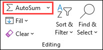
Use AutoSum
You can use AutoSum to quickly sum a column or row or numbers. Select a cell next to the numbers you want to sum, click AutoSum on the Home tab, press Enter (Windows) or Return (Mac), and that’s it!
When you click AutoSum, Excel automatically enters a formula (that uses the SUM function) to sum the numbers.
Note: You can also type ALT+= (Windows) or ALT+ += (Mac) into a cell, and Excel automatically inserts the SUM function.
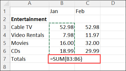
Here’s an example. To add the January numbers in this Entertainment budget, select cell B7, the cell immediately below the column of numbers. Then click AutoSum. A formula appears in cell B7, and Excel highlights the cells you’re totaling.
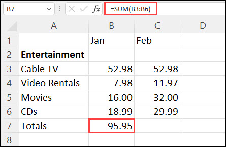
Press Enter to display the result (95.94) in cell B7. You can also see the formula in the formula bar at the top of the Excel window.
Notes:
-
To sum a column of numbers, select the cell immediately below the last number in the column. To sum a row of numbers, select the cell immediately to the right.
-
Once you create a formula, you can copy it to other cells instead of typing it over and over. For example, if you copy the formula in cell B7 to cell C7, the formula in C7 automatically adjusts to the new location, and calculates the numbers in C3:C6.
-
You can also use AutoSum on more than one cell at a time. For example, you could highlight both cell B7 and C7, click AutoSum, and total both columns at the same time.
Copy the example data in the following table, and paste it in cell A1 of a new Excel worksheet. If you need to, you can adjust the column widths to see all the data.
Note: For formulas to show results, select them, press F2, and then press Enter (Windows) or Return (Mac).
|
Data |
||
|
2 |
||
|
5 |
||
|
Formula |
Description |
Result |
|
=A2+A3 |
Adds the values in cells A1 and A2 |
=A2+A3 |
|
=A2-A3 |
Subtracts the value in cell A2 from the value in A1 |
=A2-A3 |
|
=A2/A3 |
Divides the value in cell A1 by the value in A2 |
=A2/A3 |
|
=A2*A3 |
Multiplies the value in cell A1 times the value in A2 |
=A2*A3 |
|
=A2^A3 |
Raises the value in cell A1 to the exponential value specified in A2 |
=A2^A3 |
|
Formula |
Description |
Result |
|
=5+2 |
Adds 5 and 2 |
=5+2 |
|
=5-2 |
Subtracts 2 from 5 |
=5-2 |
|
=5/2 |
Divides 5 by 2 |
=5/2 |
|
=5*2 |
Multiplies 5 times 2 |
=5*2 |
|
=5^2 |
Raises 5 to the 2nd power |
=5^2 |
Need more help?
You can always ask an expert in the Excel Tech Community or get support in the Answers community.
Need more help?
Want more options?
Explore subscription benefits, browse training courses, learn how to secure your device, and more.
Communities help you ask and answer questions, give feedback, and hear from experts with rich knowledge.
Excel is full of formulas. Those who master those formulas are pros of Excel. However, at the start of learning Excel, everyone is curious to know how to apply or create formulas in Excel. If you are one of them who is willing to learn how to create formulas in Excel, then this article is best suited for you. This article will have a complete guide from zero to intermediate level formula application in Excel.
Let us create a simple calculator-type formula for adding up numbers to start with Excel formulas.
You can download this Create a Formula Excel Template here – Create a Formula Excel Template
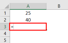
Look at the below data of numbers.
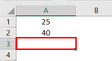
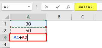
In cell A1, we have 25. The A2 cell has 40, the number.
In cell A3, we need the summation of these two numbers.
In Excel, to start the formula, always put the equal sign first.
Now, insert 25 + 40 as the equation.
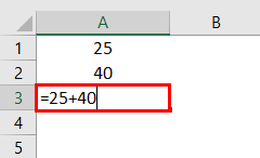
It is very similar to what we do in the calculator.
Press the “Enter” key to get the total of these numbers.

So, 25 + 40 is 65, the same we got in cell A3.
Table of contents
- How to Create a Formula in Excel?
- #1 Create Formula Flexible with Cell References
- #2 Use SUM Function to Add Up Numbers
- #3 Create Formula References to Other Cells Excel
- Recommended Articles
#1 Create Formula Flexible with Cell References
Let us start.
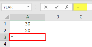
- From the above example, we will change the number from 25 to 30 and 40 to 50.

Even though we have changed numbers in cells A1 and A2, our formula only shows the old result of 65. It is a problem with direct numbers passing to the formula. It does not make the formula flexible enough to update the new result.
- We can give cell reference as the formula reference to overcoming this issue. For example, open the equal sign in cell A3.

- Then, select cell A1.

- Insert plus (+) sign and select cell A2.

- Press the “Enter” key to get the result.


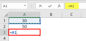
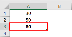
As we can see in the formula bar, it is not showing the result. Rather, it shows the formula itself, and cell A3 shows the result of the formula.
Now, we can change the numbers in A1 and A2 cells to see the immediate impact of the formula.
#2 Use SUM Function to Add Up Numbers
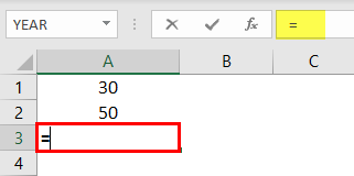
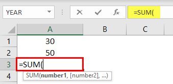
To get used to the formulas in Excel, let us start with the simple SUM function. All the formulas should begin with “+” or “=.” So, open the equal sign in cell A3.
Start typing the SUM to see the intellisense list of Excel functionsExcel functions help the users to save time and maintain extensive worksheets. There are 100+ excel functions categorized as financial, logical, text, date and time, Lookup & Reference, Math, Statistical and Information functions.read more.
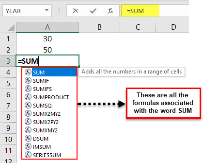
Press the “Tab” key once the SUM formula is selected to open the SUM function in excel.The SUM function in excel adds the numerical values in a range of cells. Being categorized under the Math and Trigonometry function, it is entered by typing “=SUM” followed by the values to be summed. The values supplied to the function can be numbers, cell references or ranges.read more
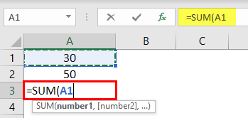
The first argument of the SUM function is Number 1, whichis the first number we need to add. In this example, cell A1. So, we must select cell A1.
The next argument is Number 2, the second number or item we need to add, A2 cell.
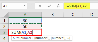
Now, we must close the bracket and press the “Enter” key to see the result of the SUM function.
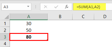
Like this, we can create simple formulas in Excel to do the calculations.
#3 Create Formula References to Other Cells Excel
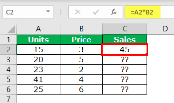
We have seen the basics of creating a formula in Excel. Similarly, we can apply one formula to other related cells as well. For example, look at the below data.
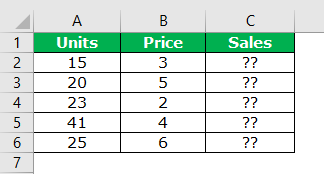
In column A we have “Units.” In column B, we have the “Price Per Unit.”
In the column, C needs to arrive at “Sales Amount.” For arriving at the sales amount, the formula is Units * Price.
- So, we must open an equal sign in cell C2.
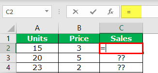
- Select cell A2 (units).
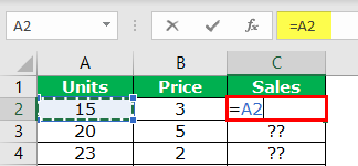
- Enter multiple sign (*) and select the B2 cell (price).
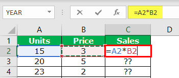
- Press the “Enter” key to get the sales amount.
Now, we have applied the formula in cell C2. How about the remaining cells?
Can you enter the same formula for the remaining cells individually?
If you think that way, you will be delighted to hear that the “formula is to be applied to a single cell, then we can copy-paste to other cells.”
Now first, look at the formula we have applied.
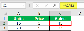
The formula says A2 * B2.
So, when we copy and paste the formula below, cell A2 becomes A3, and B2 becomes B3.
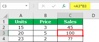
Similarly, row numbers keep changing as we move down, and column letters will also change if we move either left or right.
- Copy and paste the formula to other cells to result in all the cells.
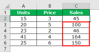
Like this, we can create a simple formula in Excel to start your learning.
Recommended Articles
This article has been a guide to creating a formula in Excel. Here, we learn to create a simple Excel formula and practical examples, and a downloadable template. You may learn more about Excel from the following articles: –
- Write Formula in Excel
- PI in Excel
- Excel Formula Not Working
- List of Basic Excel Formulas
Чаще всего под формулами в Excel подразумевают именно встроенные функции, предназначенные для выполнения расчетов, и куда реже математические формулы, имеющие уже устоявшийся вид.
В этой статье я рассмотрю обе темы, чтобы каждый пользователь нашел ответ на интересующий его вопрос.
Окно вставки функции
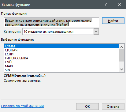
Некоторые юзеры боятся работать в Экселе только потому, что не понимают, как именно устроены функции и каким образом их нужно составлять, ведь для каждой есть свои аргументы и особые нюансы написания. Упрощает задачу наличие окна вставки функции, в котором все выполнено в понятном виде.
-
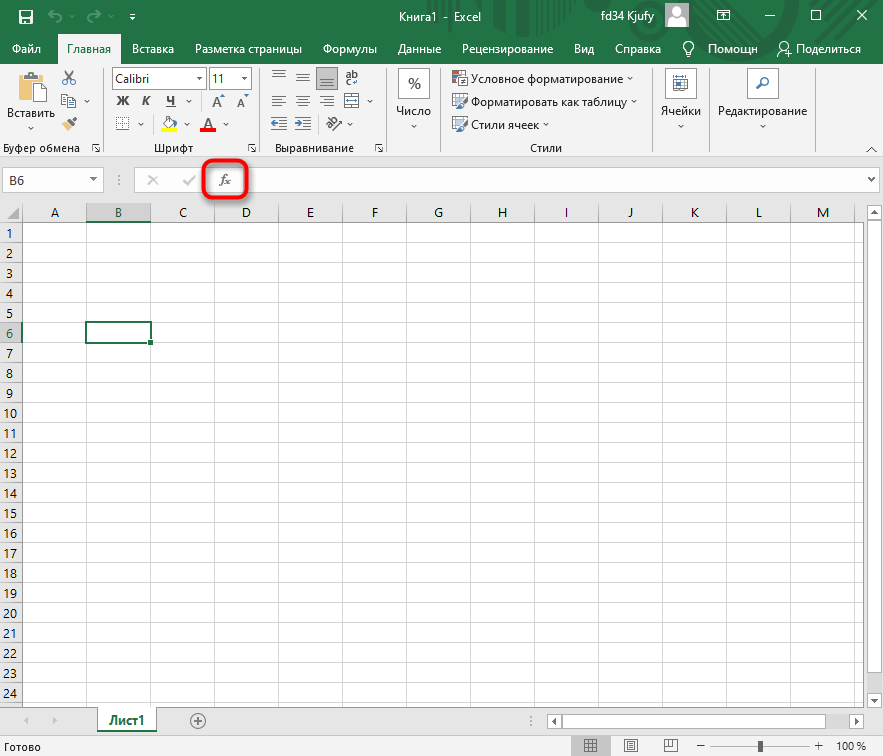
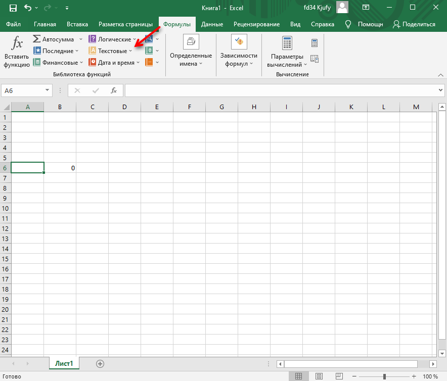
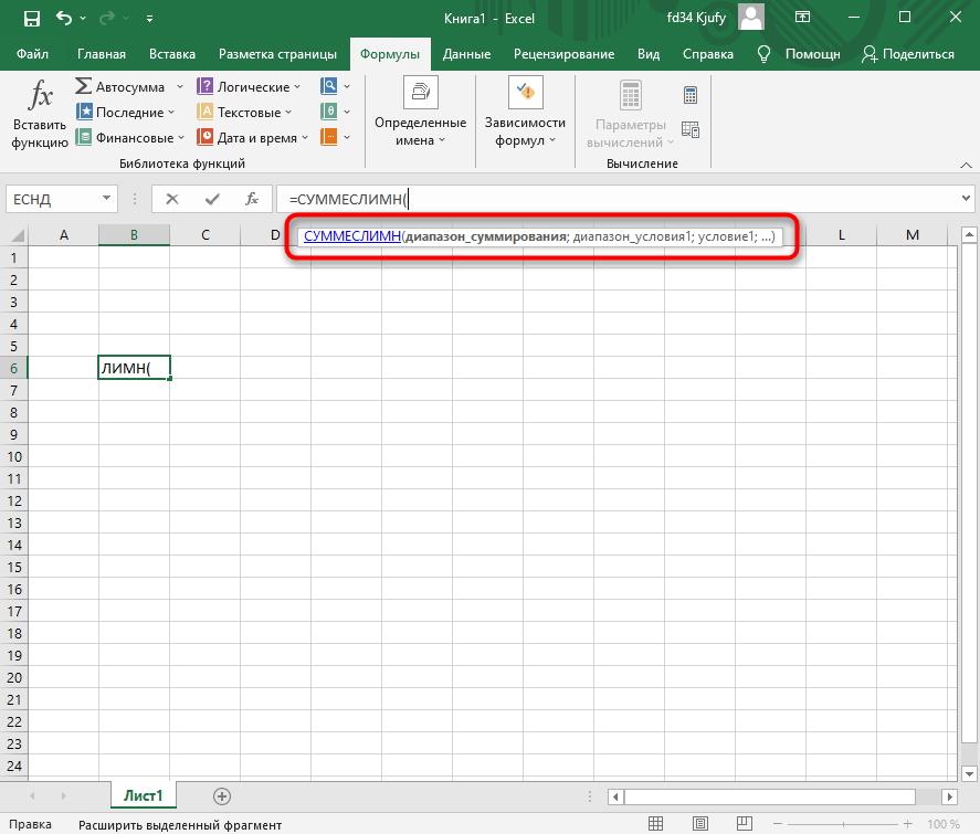
Для его вызова нажмите по кнопке с изображением функции на панели ввода данных в ячейку.

-
В нем используйте поиск функции, отобразите только конкретные категории или выберите подходящую из списка. При выделении функции левой кнопкой мыши на экране отображается текст о ее предназначении, что позволит не запутаться.
-
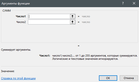
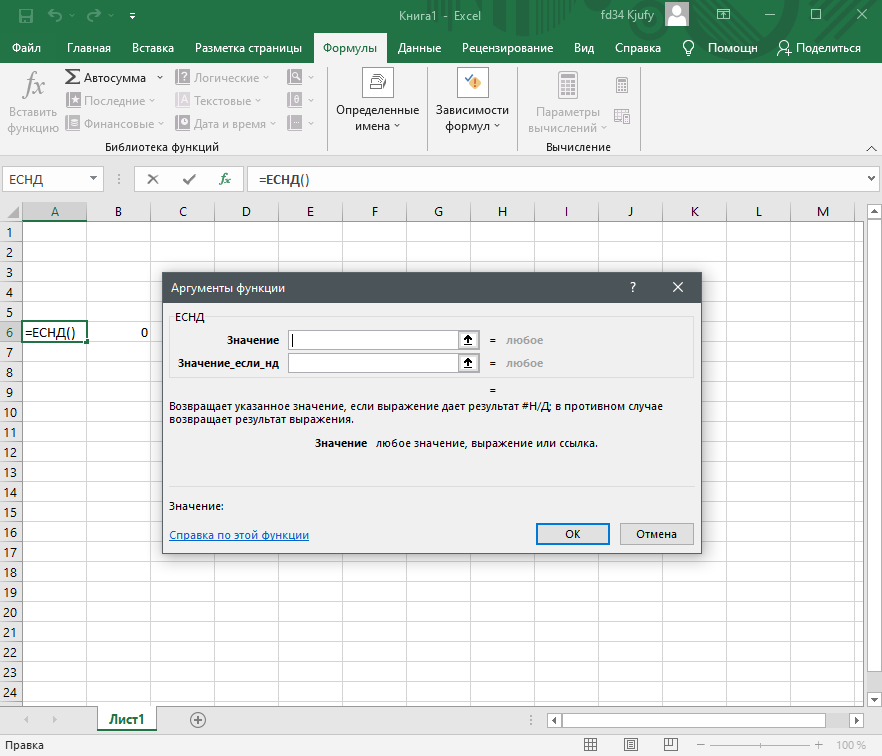
После выбора наступает время заняться аргументами. Для каждой функции они свои, поскольку выполняются совершенно разные задачи. На следующем скриншоте вы видите аргументы суммы, которыми являются два числа для суммирования.
-
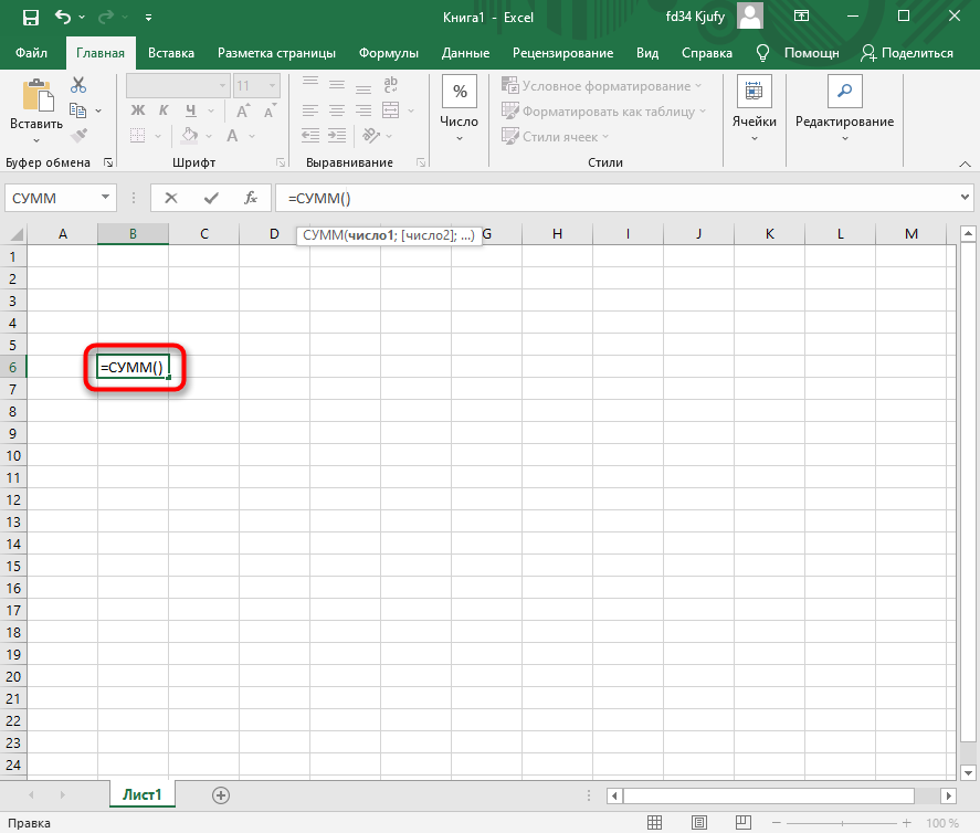
После вставки функции в ячейку она отобразится в стандартном виде и все еще будет доступна для редактирования.
Комьюнити теперь в Телеграм
Подпишитесь и будьте в курсе последних IT-новостей
Подписаться
Используем вкладку с формулами
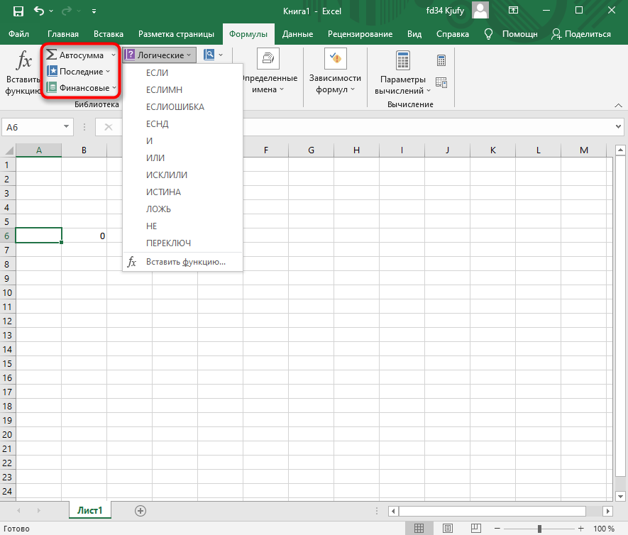
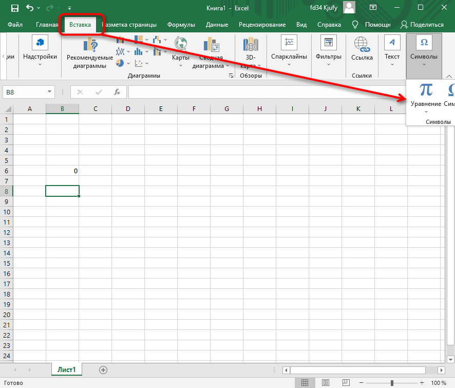
В Excel есть отдельная вкладка, где расположена вся библиотека формул. Вы можете использовать ее для быстрого поиска и вставки необходимой функции, а для редактирования откроется то же самое окно, о котором шла речь выше. Просто перейдите на вкладку с соответствующим названием и откройте одну из категорий для выбора функции.
Как видно, их названия тематические, что позволит не запутаться и сразу отобразить тот тип формул, который необходим. Из списка выберите подходящую и дважды кликните по ней левой кнопкой мыши, чтобы добавить в таблицу.
Приступите к стандартному редактированию через окно аргументов функции. Кстати, здесь тоже есть описания, способные помочь быстрее разобраться с принципом работы конкретного инструмента. К тому же ниже указываются доступные значения, которые можно использовать для работы с выбранной формулой.
Ручная вставка формулы в Excel
Опытные пользователи, работающие в Excel каждый день, предпочитают вручную набирать формулы, поскольку так это делать быстрее всего. Они запоминают синтаксис и каждый аргумент, что не только ускоряет процесс, но и делает его более гибким, ведь при использовании одного окна с аргументами довольно сложно расписать большую цепочку сравнений, суммирований и других математических операций.
Для начала записи выделите ячейку и обязательно поставьте знак =, после чего начните вписывать название формулы и выберите ее из списка.
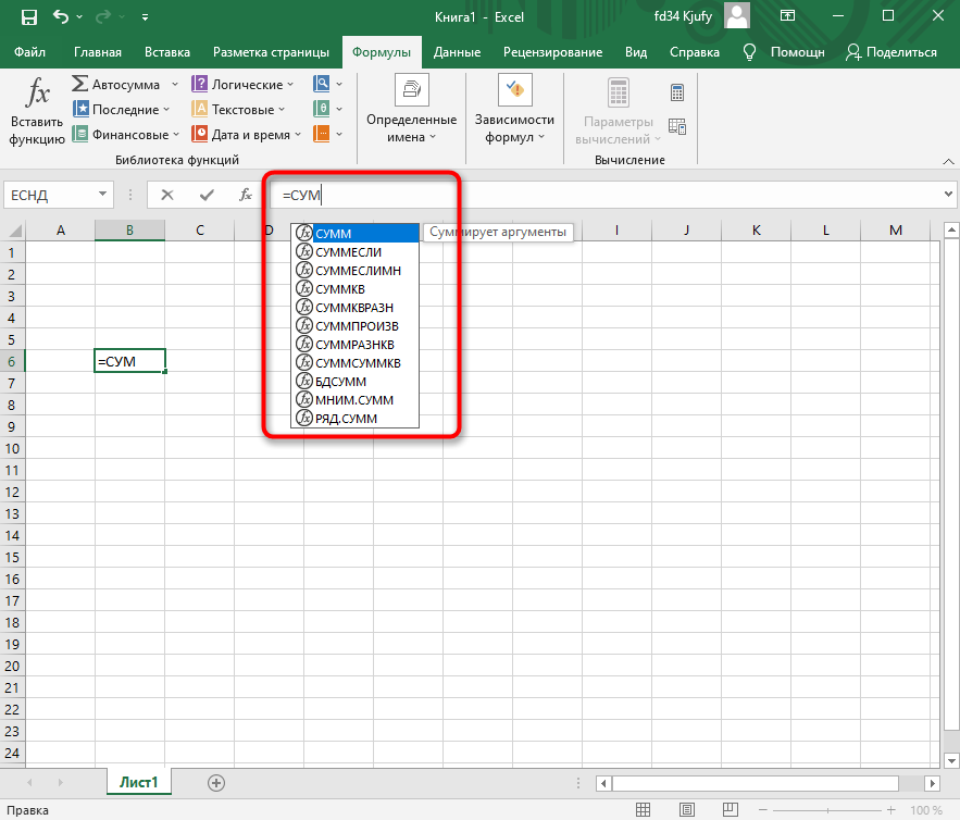
Далее начните записывать аргументы, в чем помогут всплывающие подсказки. По большей части они нужны для того, чтобы не запутаться в последовательности и разделителях.
По завершении нажмите клавишу Enter, завершив тем самым создание формулы. Если все записано правильно, и программе удается рассчитать результат, он отобразится в выбранной ячейке. При возникновении ошибки вы сможете ознакомиться с ее текстом, чтобы найти решение.
Вставка математических формул
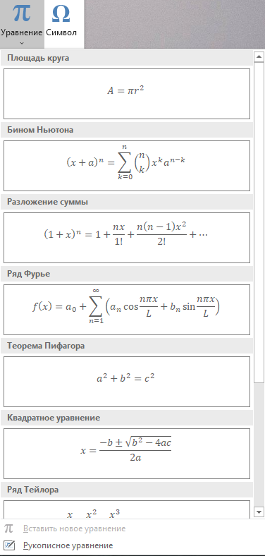
В завершение поговорим о математических формулах в Excel, так как тематика статьи подразумевает и вставку таких объектов в таблицу тоже. Доступные уравнения относятся к символам, поэтому для их поиска понадобится перейти на вкладку со вставкой и выбрать там соответствующий раздел.
Из появившегося списка найдите подходящее для вас уравнение или приступите к его ручному написанию, выбрав последний вариант.
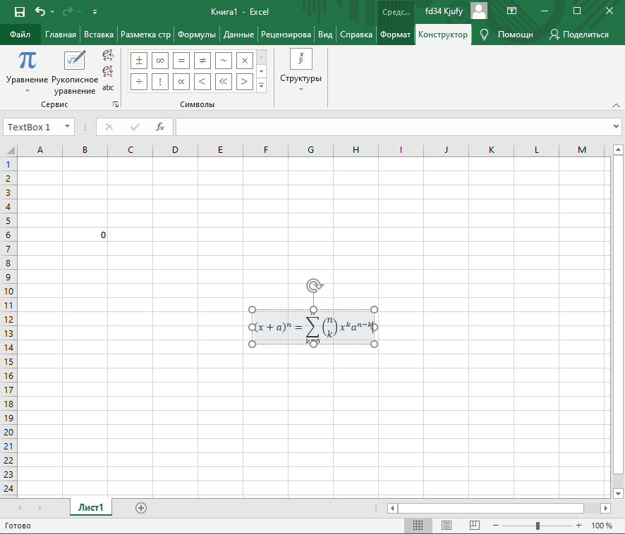
На экране появится редактор и блок формулы. Его используйте для перемещения, а сам редактор – для того, чтобы заносить в формулу числа и редактировать ее под себя. Учитывайте, что в этом случае не работают никакие проверки, поэтому правильность написания проверять придется собственноручно.
Это были самые простые способы вставить функции и формулы в Excel. Первые три помогут создать операции, а последний пригодится математикам и тем, кто выполняет сложные расчеты при помощи таблицы и нуждается во вставке математических формул.
How to Create a Formula in Excel: Beginner Tutorial (2023)
Excel is all about running calculations! And so creating and operating a formula in Excel is simple.
An Excel formula is a combination of operators and operands. For example, 2 + 2 = 4 is a formula where 2s are the operands, plus sign (+) is the operator, and 4 is the answer to the formula.
Only if you know the basics to write a formula in Excel – there’s a high chance you’d solve most of your Excel problems. This article explains the basics of creating Excel formulas.
So let’s dive right in.
As you scroll down, download our free sample workbook here to practice the examples used in the guide below. 😀
How to create formulas in Excel
Creating Excel formulas is easy as pie.
For example, what is 10 divided by 2? Can you calculate this in Excel?
1. Start by activating a cell.
2. Write an equal sign.

It is very important to start any formula with an equal sign. If you do not start with an equal sign, Excel wouldn’t recognize it as a formula but as a text string.
3. Input the simple mathematical operation of 10 divided by 2.
= 10 / 2

4. Hit enter, and you’re good to go!

You can create the same above formula with a slight variation.
For example, if you have the operands as cell values.

1. Write the formula using cell references as follows.
= A2 / B2

The above formula translates to ‘A2 divided by A3’.
Where A2 has the numeric value 10, and A3 has the numeric value 2.
2. The results remain the same as in the above example.

Creating a formula using cell references and values
The same formula can also be created using a combination of cell references and values.
Write the following formula using cell references and values.
= A2 / 2

The above formula translates to ‘A2 divided by 2’.
Where A2 has the numeric value 10, and 2 is a value.
1. The results look as follows.

Pro Tip!
Using cell references is better than using absolute values. This is because if sometime later you change the cell value – the formula would automatically update.
How to add, subtract, multiply, and divide?
There are four basic mathematical operations – add, subtract, multiply, and divide.
Let’s now see how to perform each of these operations in Excel.
How to make a SUM formula (addition)
Adding things up in Excel can take different forms.
Excel has an in-built function for performing addition i.e. the SUM function. Here’s how you can bring it to action.
1. Write the SUM function beginning with an equal sign as follows.
= SUM (5, 5)
Every argument of the SUM function separated by a comma represents the value to be added.
Excel adds 5 into 5 to give the results below.

Easy enough? You can use the SUM function for cell references too. 🤩
2. Write the SUM function as follows.
= SUM (A2, A3)
Pro Tip!
To insert SUM from the Insert Function button, take this route.
Go to Formulas tab > Function Library > Insert function button > Type the function name.
In the Insert Function dialog box, type SUM and hit search. Select the desired function and hit ‘Okay’ to insert the same.
Excel adds the cell values of Cell A2 and Cell A3.

What makes the SUM function a big plus is its ability to add up a range of cells.
For example, see the data below.

3. To add this up in Excel using the SUM function, write the SUM function as below.
= SUM (A2:A10)

Must notice how we have defined the cell range from Cell A2 to Cell A10 as A2:A10.
4. Excel sums up all cell values in cells from A2 to A10.

You can make this function work even more interestingly by adding up multiple ranges.
5. Write the SUM function with multiple ranges as follows.
= SUM (A2:A5, B2:B8, C1:C10)


How to subtract in Excel
Subtracting in Excel is all about creating a formula with the minus sign operator (-).
For example:
1. To subtract 5 from 10, begin with an equal sign and write the following formula.
= 10 – 5
A simple subtraction formula with a minus sign operator!
Press enter and here you go.

2. Try doing the same with cell references as below.
= A2 – A3
This formula translates to A2 less A3. Where A2 has the numeric value 10, and A3 has the numeric value 5.

3. Alternatively, you can use the SUM function to perform subtraction. However, to do this you need to add a minus sign to the value to be subtracted.
= SUM (A2, -A3)
Here are the results.

How to multiply in Excel
After we have learned how to add and subtract in Excel, it’s time we learn multiplication in Excel.
First thing first, the operator for multiplication in Excel is an asterisk (*).
Now, do you remember what is 9 times 8? No?
1. Write a multiplication formula in Excel.
= 9 * 8


2. Try doing the same using cell references as below.
= A2 * A3

The formula above translates to A2 multiplied by A3.
Excel also offers an in-built function for multiplication in Excel. The PRODUCT Function!
3. Write the PRODUCT function as follows.
= PRODUCT (9, 

We have added both the values to be multiplied as the arguments to the PRODUCT function.
Here are the results.

The PRODUCT function can also find the product of multiple values (or a range of cells) at once.
For example, see the data below.

4. To multiply all these values, write the PRODUCT function as follows:
= PRODUCT (A2:A10)

Excel multiplies all the values in the specified range.

How to divide in Excel
Here comes the last operation of this guide – division. 🤞
Creating a division formula in Excel is also very straightforward.
What is the operator for division? A forward slash (/).
Also, the dividend (or the numerator) comes before the slash. And the divisor (or the denominator) comes after the slash.
1. Write a division formula as below.
= 30 / 10

Excel divides both operands to give the results as follows.

2. The same can be done using cell references.
= A2 / A3
Pro Tip!
While performing the division function in Excel, you might see the #DIV/0! Error. This error is given back by Excel when you attempt to divide the number of zero.
Basic Rule of Grade 6! No number is divisible by zero. Excel remembers that, if not us. 😆
Order of operations
Here’s an equation for you to solve.
= 2+ 4 * 6 / 3 – 2
What a mess! Which operation do you perform first?
To solve this mystery, there is an order for performing mathematical operations – PEMDAS
P = Parenthesis
E = Exponents
MD = Multiplication & Division (left to right)
AS = Addition & Subtraction
Solve the above equation in the same order, and you’d reach the answer 8.
Let Excel do the same to see the results.

Excel performs division first (6 / 3 = 2), multiplication second (4 * 2 = 8), addition third (2 + 8 = 10), and subtraction last (10 – 2 = 8), resulting in 8.
Now, let’s enclose a part of this formula in parentheses to see how the results change.
= 2+ 4 * 6 / (3 – 2)

What causes the results to change with only parenthesis added?
Excel now first performs the operation enclosed in parenthesis i.e. (3-2).
Next, multiplication is performed, then division and addition last. This causes the answer to change.
Pro Tip!
Try doing some mental maths to double-check if Excel has rightly calculated 26.
Parenthesis first = 2+ 4*6/(3 – 2)
Multiplication Second= 2+4*6/1
Division Third = 2 + 24/1
Addition Last = 2 + 24
Here’s the answer = 26
How to create formulas with references
Creating Excel formulas with references is super simple. All you need to do is replace the values in a simple formula with cell references (cells that contain those values).
For example, let’s create a multiplication formula in Excel.

Great! What if you had 2 & 4 as numerical values in cells?

Create the same formula using cell references.

You can do the same for all operators! It is this simple.
Also, what happens when a cell value changes? Until the cell reference is in place, the formula would automatically update for the cell value change.

Must note how the cell reference in the formula remains unchanged. The answer however changes as the cell value for A3 has changed.ltiple criteria lookup💡
Formulas or functions?
What is an Excel formula, and what is an Excel function? And how are these two different?
There are two ways to add 2 and 2 in Excel.
- = 2 + 2
- SUM (2,2)
The answer to them both would be the same. However, the first one is a formula created in Excel. Whereas the second one is an in-built function of Excel – the SUM function.
Functions are more like predefined formulas in Excel.
Although the function library of Microsoft Excel is huge enough for you to explore, there is a limit to it. And you may not find everything you need there.
So, you might still need to write your own formulas to perform calculations in Excel. 😉
Pro Tip!
Sometimes, you might even nest a function into a formula.
For example, what is 2 + 2 – 3?
You may write it as = (SUM (2,2)) – 3
SUM (2,2) is a function, and deducting 3 from it makes it a self-created formula.
That’s it – Now what?
Until now, we’ve created formulas using different operators, values, and cell references. And learned how to use the SUM function for addition and subtraction.
Not only that but we’ve also studied the order of operations in Excel. The above article is a whole pack of information, isn’t it?
Creating your own formulas in Excel is the first step to manipulating numbers in Excel. However, this is something very basic, and Excel has tons more to offer.
Some very important Excel functions that one must hone include the VLOOKUP, SUMIF, and IF functions.
Haven’t mastered them yet? Click here to register for my 30-minute free email course that helps you learn these and much more.
Kasper Langmann2023-02-23T14:38:38+00:00
Page load link
Spreadsheets aren’t merely for arranging data into rows and columns. Most of the time, you use them for data analysis as well.
Microsoft Excel is one of the most widely used spreadsheet applications, especially in finance and accounting. This is partly because of its easy UI and unmatched depth of functions.
In this article, you will learn:
- What Excel formulas are
- How to write a formula in Excel
- What Excel functions are
- How to work with an Excel function
- Lastly, we’ll take a look at dynamic Excel functions.
What do I need to install on my computer to follow this article?
To follow along, you will need to have Microsoft Excel installed on your computer. We’ll use a Windows computer for this article.
How can I install Microsoft Excel on my computer?
Follow these steps to install Microsoft Excel on your Windows computer:
- Sign in to www.office.com if you’re not already signed in.
- Sign in with the account associated with your Microsoft 365 subscription. You can also try out Office for free as well.
- Once signed in, select “Install Office” from the Office home page. This will automatically download Microsoft Office onto your Windows computer.
- Run the installer to set up Microsoft Office and select «Close» once you’re done.
- Once done, select the “Start” button (located at the lower-left corner of your screen) and type “Microsoft Excel.”
- Click on Microsoft Excel to open it.
- Accept the license agreement, and let’s get started.
What are Excel Formulas?
An Excel formula is an expression that carries out an operation based on the value of a cell or range of cells. You can use an Excel formula to:
- Perform simple mathematical operations such as addition or subtraction.
- Perform a simple operation like joining categorical data.
It’s important to understand two things: Excel formulas always begin with the equals «=» sign and they can return an error if not properly executed.
What Operators Are Used in Excel Formulas?
There are four different types of operators in Excel—arithmetic, comparison, text concatenation, and reference. But for most formulas, you’ll typically use these three:
Arithmetic operators
|
+ |
Addition |
|
— |
Subtraction |
|
/ |
Division |
|
* |
Multiplication |
|
^ |
Exponentiation |
Comparison operators
|
= |
Equal to |
|
> |
Greater than |
|
< |
Less than |
|
>= |
Greater than or equal to |
|
<= |
Less than or equal to |
|
<> |
Not equal to |
Text concatenation
Here you have just the ampersand “&” sign for joining text.
How Can I Create an Excel Formula?
Let’s take a simple scenario using one of the arithmetic operators.
In math, to add up two numbers, let’s say 20 and 30, you will calculate this by writing: 20 + 30 =
And this will give you 50.
In Excel, here is how it goes:
- First, open a blank Excel worksheet.
- In cell A1, type 20.
- In cell A2, type 30.
- To add it up, type in = 20 + 30 in cell A3.

5. Then, press ENTER on your keyboard. Excel will instantly calculate this and return 50.

I mentioned earlier that every formula begins with the equal «=» sign. That’s what I meant. To write a formula, you type the equal to sign followed by the numeric values. This also applies to cases of subtraction, division, multiplication, and exponentiation.
Let’s take another simple scenario using one of the comparison operators. Assume we want to find out if 30 is greater than 40.
In Excel, here is how we would do it:
- Type in =30>40
- Press ENTER.

3. This will return a FALSE because 30 isn’t greater than 40. Excel uses TRUE and FALSE for logical statements, the same way we human says yes and no.

Lastly, let’s take another simple scenario using the text concatenation operator – the ampersand “&” sign. This works with your string data types and you use it to join text.
Assume we have «Welcome», «To», and «FreeCodeCamp» all in different cells—A1, A2, and A3—of your worksheet. We would type =A1&” “&A2&” “&A3 to join them.
The space in quotes “ “ represents that we want a space between our words.

Another tip: the formula bar shows the formula used to generate a value.
What Are Excel Functions?
Excel functions are predefined inbuilt formulas that perform mathematical, statistical, and logical calculations and operations using your values and arguments.
For Excel functions, you should know that:
- They’re formulas, so yeah, they start with the equal «=» sign as well.
- The order is very important.
There are over 500 functions available. You can find all available Excel functions on the Formulas tab on the Ribbon.

But why use a function when you can just write a formula?
Here are some benefits of Excel functions.
- To improve productivity and effectiveness.
- To simplify complex calculations.
- To automate your work.
- To quickly visualize data.
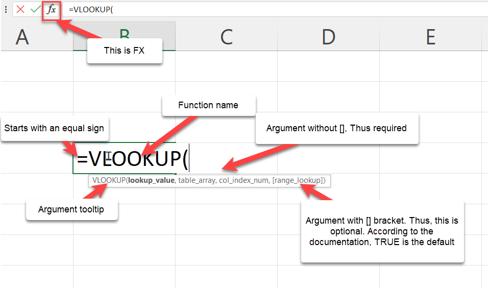
What Makes Up Excel Functions?
Unlike formulas, Excel functions are made up of a structure with arguments you need to pass.
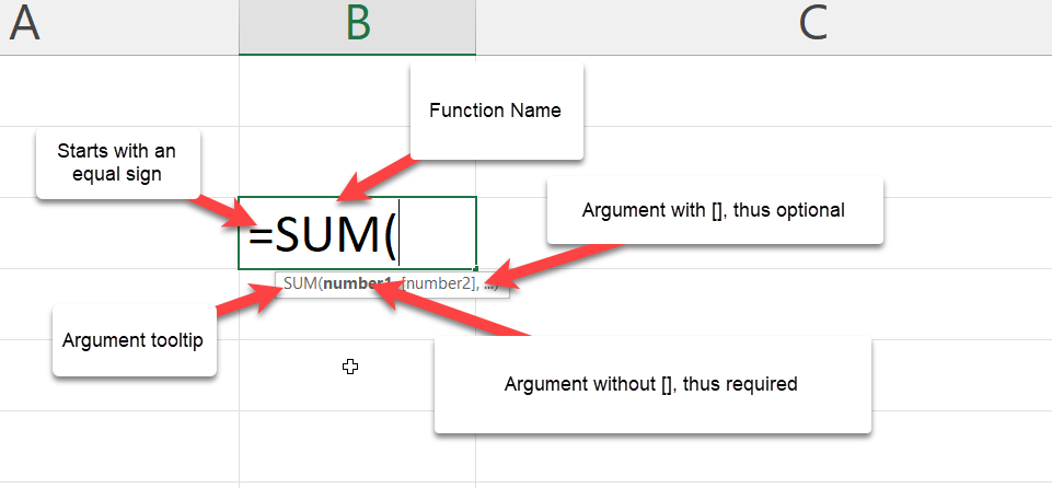
Every function:
- Starts with the equals «=» sign
- Has a name. Some examples are VLOOKUP, SUM, UNIQUE, and XLOOKUP.
- Requires arguments which are separated by commas. You should know that semicolons are used as separators in countries like Spain, France, Italy, Netherlands, and Germany. You can, however, change this via the Excel setting.
- Argument with the square brackets [] are optional
- Has an opening and closing parenthesis.
- Has an argument tooltip which shows you what you should pass.
There are some exceptions. For example,
- The DATEDIF doesn’t show in Excel because it is not a standard function and gives incorrect results in a few circumstances. However, here is the syntax:
DATEDIF(birthdate, TODAY(), "y")
- Functions like PI(), RAND(), NOW(), TODAY() require no argument.
Let’s look at a few functions:
How to Use the SUM() Function in Excel
According to the documentation, the SUM function adds values. Here is the syntax:
Let’s assume that we have a line of numbers from 1 to 10 and we want to add it up. To achieve this, we will just type =SUM(A1:A10). The A1:A10 simply returns an array of number that are situated on cell A1 to A10 which are A1, A2, and A3 up through A10.

Since the second argument is optional, that means a sum(A10) will return a value. In our case, it will return just 10 since A10 has the value 10 in it. Give it a try.
If you were writing this using the addition operator, you would have written:
=1 + 2 + 3 + 4 + 5 + 6 + 7 + 8 + 9 + 10
or
=A1 + A2 + A3 + A4 + A5 + A6 + A7 + A8 + A9 + A10
This doesn’t look very productive or efficient.
How to Use the TODAY() Function in Excel
According to the documentation, the TODAY function displays the current date on your worksheet. It also requires no argument. Here is the syntax:

Excel displays the current date automatically according to your computer’s date and time setting. The same goes for the NOW() function, which displays the current date and time.
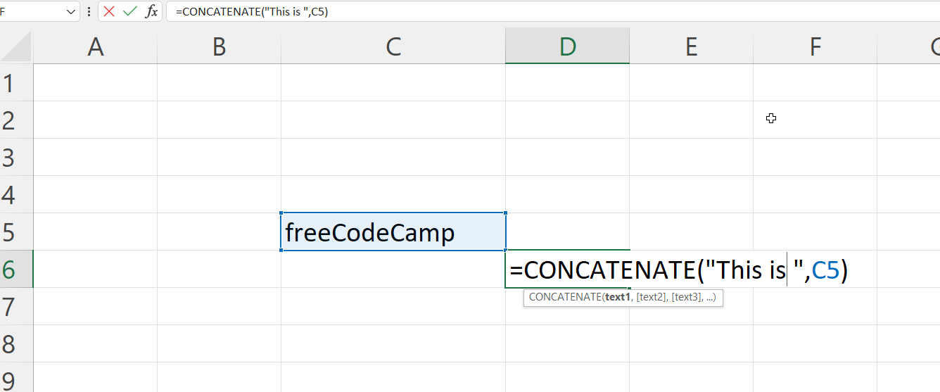
How to Use the CONCATENATE() Function in Excel
Let’s look at a text function. You use CONCATENATE to join two or more text strings into one string together.
Here is the syntax:

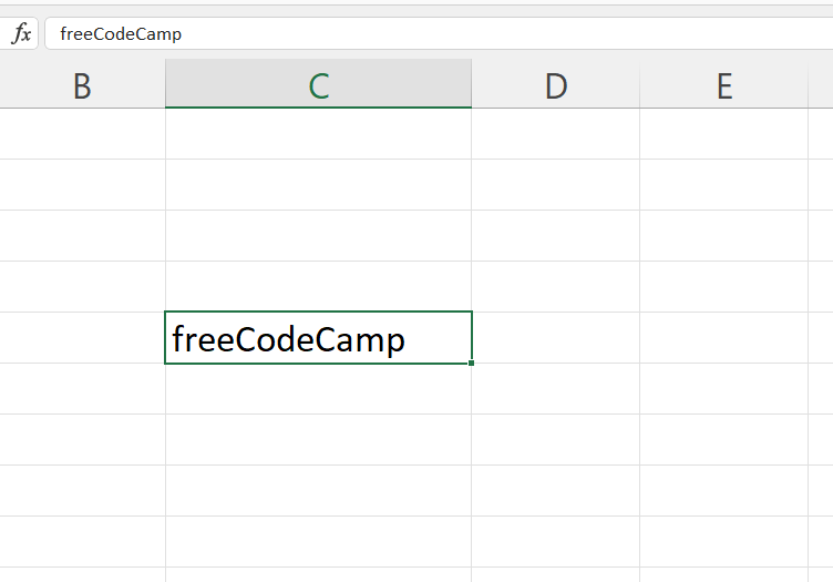
Let’s assume we want to join “This is” with “freeCodeCamp” – but in your cell, you have just «freeCodeCamp.»
If you’re going to write a string inside a formula, you must write it inside quotes like this “ “.
Why?
This way, Excel wouldnt think you’re trying to write another function.
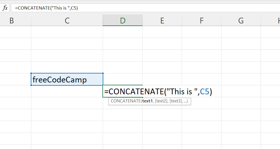
This will return the phrase “This is freeCodeCamp”
How to Use the VLOOKUP() Function in Excel
This is one of Excel’s most interesting and commonly used formulas or functions. You use it to find a value in a table or range by row.
Here is a scenario:
We have a simple table that shows various films along with their genre, lead studio, audience score %, profitability, rotten tomatoes %, worldwide gross and year. I would use just the first 10 rows of the sample data from this GitHub Gist.

I want that, whenever I type in a movie in the yellow cell, the year should get displayed in the green cell. Let’s use VLOOKUP to find it.
This is the VLOOKUP syntax:
Besides writing your formulas in the cell, you can also write them using the Excel Insert Function (fx) button, which is close to the formula bar.
Let’s try this.
- Write
=Vlookup(on the green cell. - Click on fx. A dialogue box will pop up showing all the arguments this formula needs.
- Input the value for each argument.
- Lookup_value (required argument): This is what you want to find. In our case, that is the movie “Youth in Revolt” which is in cell B1.
- Table_array (required argument): This is just asking you for the table that contains the data. You give it the entire table, which in our case is A4:H13
- Col_index_num (required argument): This is asking you for the column number of the table you gave. In our case, we want the year. This is in column 8.
- Range_lookup (optional argument): Lastly, we pick if we want an approximate match (TRUE) or an exact match (FALSE).
— TRUE means approximate match, so it returns the closest or an estimate.
— FALSE means exact match, so it returns an error if it’s not found.
8. We would go for the FALSE because we want the exact match.

9. Click on «OK.» Excel will return 2010.
However, you can write this in the cell by typing in =VLOOKUP(B1,A4:H13,8,FALSE) in your cell.

Tips and Rules When Writing Excel Functions
When writing our function, Excel provides some formula tips.
- The Argument tooltip doesn’t leave until you close the last parenthesis.
- The formula bar shows your formula.
- The argument you are currently writing is always dark. Take a look at the lookup_value in the image below.
- The square brackets [] tell you it is optional.
- Lastly, the colour code – our B1 is in blue, and cell B1 is in blue to guide us on what cell or table was picked. The same thing will happen to A4:H13 when we pick it as our table_array argument.

How to Work with Nested Functions in Excel
A nested function is when you write a function within another function. For example, finding the average of the sum of values.
The first tip when writing a nested function will be to treat every function individually. So address the first function before addressing the second. A pro tip would be to look at the argument tooltip when writing it.
Let’s take a simple scenario.
We have two arrays of numbers. Each has the scores of students in the class. I want to add the two arrays before I get the average.
Let’s get started.
- Type in your = followed by the average.
- The number one will be the sum of the scores from class one.
- The number two will be the sum of the scores from class two.
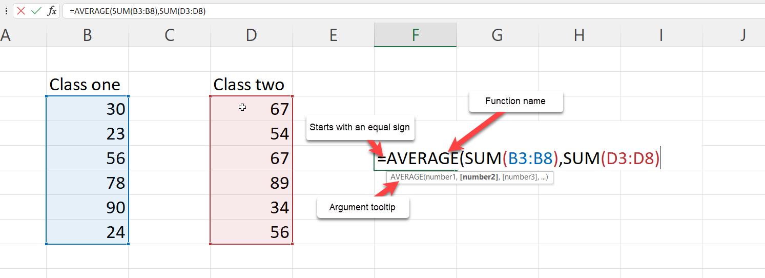

Finally, don’t forget the closing parenthesis.
Thus, the formula will be =AVERAGE(SUM(B3:B8),SUM(D3:D8)).
How to Work with Dynamic Array Functions in Excel
Dynamic array functions are formulas associated with spill array behaviour.
Before now, you wrote a function and it returned just a single input. We call these kinds of functions legacy array formulas.
Dynamic array functions, on the other hand, will return values that will enter the neighbouring cells. A few examples of dynamic array functions are:
- UNIQUE
- TEXTSPLIT
- FILTER
- SEQUENCE
- SORT
- SORTBY
- RANDARRAY
Let’s look at the UNIQUE formula.
How to Use the UNIQUE() Formula in Excel
The unique formula works by returning the unique value from an array or list. Let’s use the movie sample data from this GitHub Gist. This table contains 77 rows of film excluding the heading.

Let’s try to get the unique years from our dataset – that is, years without duplicates.
To do this:
- Type
=UNIQUE( - Select the entire array of values from the year column: =UNIQUE(H2:H78)

3. Close the parenthesis and press Enter.
Though the formula was written in a single cell, the returned value got spilled into the cells below it. That’s the spilled array behaviour.

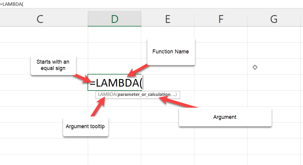
How to Create Your Own Functions in Excel
Microsoft Excel released a bunch of new functions to make user more productive. One of these function was the LAMBDA function.
The LAMBDA function lets you create custom functions without macros, VBA or JavaScript, and reuse them throughout a workbook.
The best part? you can name it.
How to Use the LAMBDA() Function in Excel
This LAMBDA function will increase productivity by eliminating the need to copy and paste this formula, which can be error-prone.
Here is the LAMBDA syntax:
Lets start with a simple use case using the movie sample data from this GitHub Gist.
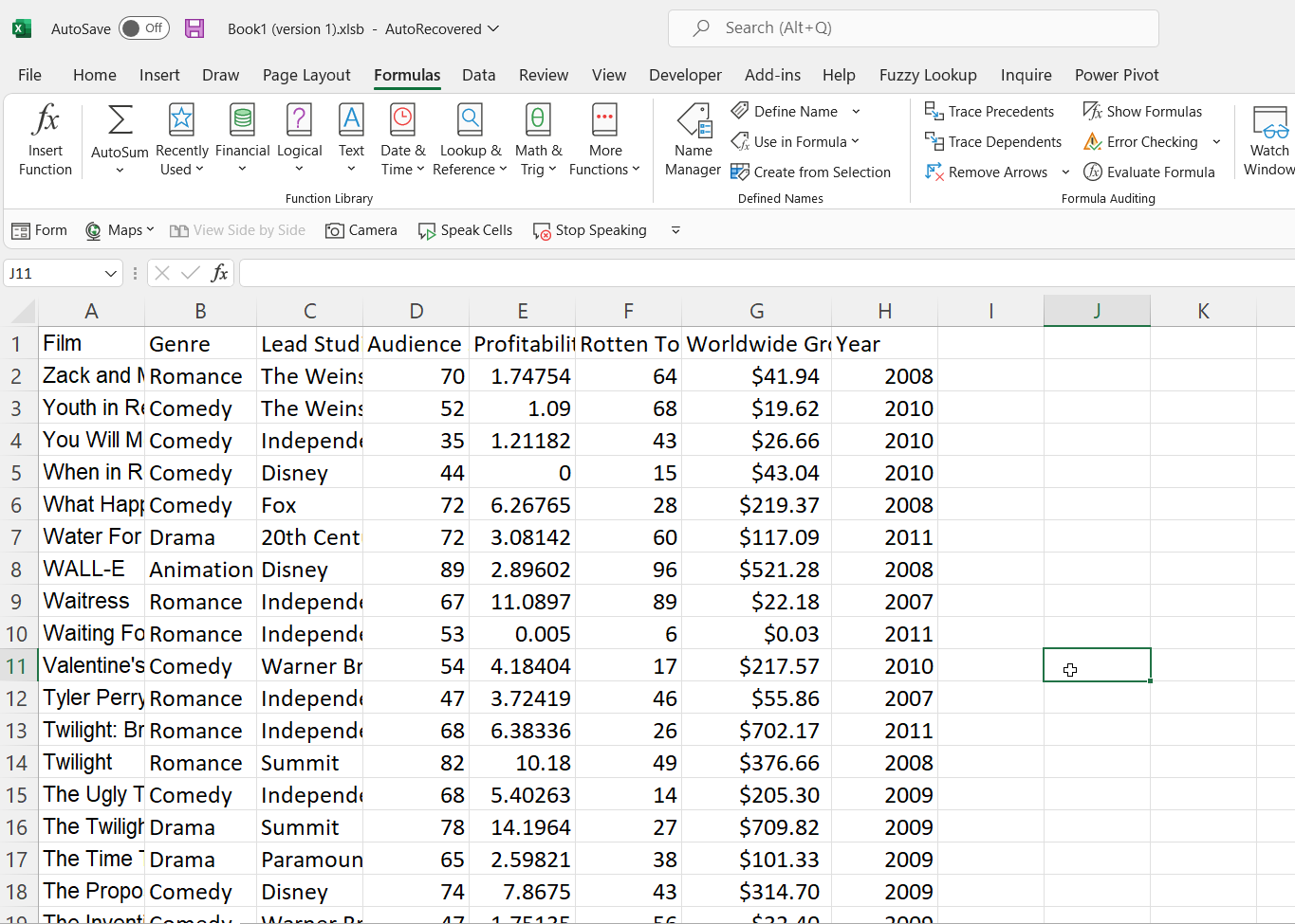
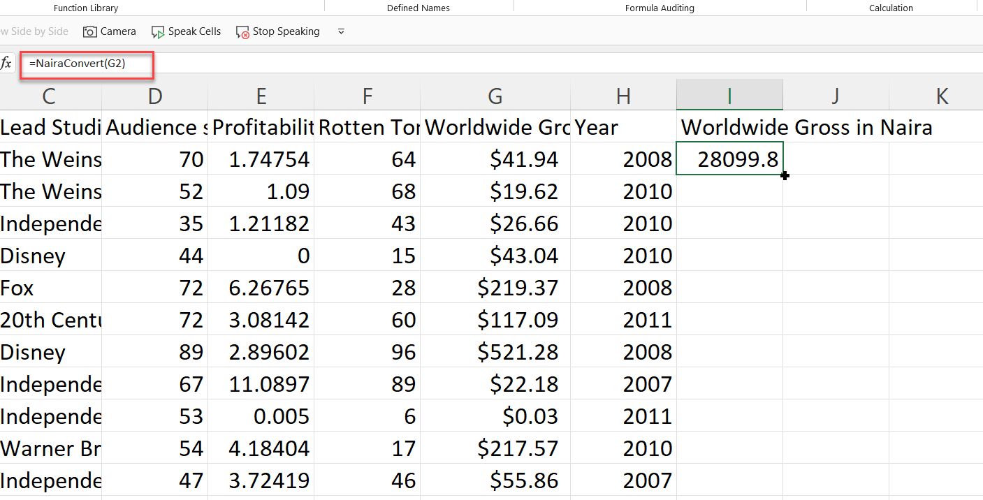
We had a column called «Worldwide Gross», lets try to find the Naira value.
- Create a new column and call it «Worldwide Gross in Naira».
- Right below our column name, Cell I2, type
=lAMBDA( - LAMBDA requires a parameter and/or a calculation.
The parameter means the value you want to pass, in our use case we want to change the gross value. Lets call it gross.
The calculation means the formula or function you want to execute. For us, that will be to multiply it with te exchange rate. At the moment, that’s 670. so lets write gross * 670.
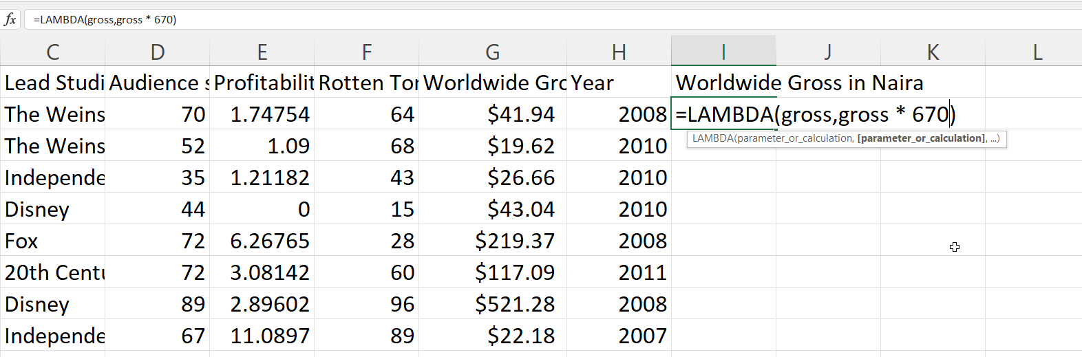
4. Press Enter. This will return an error because, gross doesnt exist and you need to let excel know of these names.
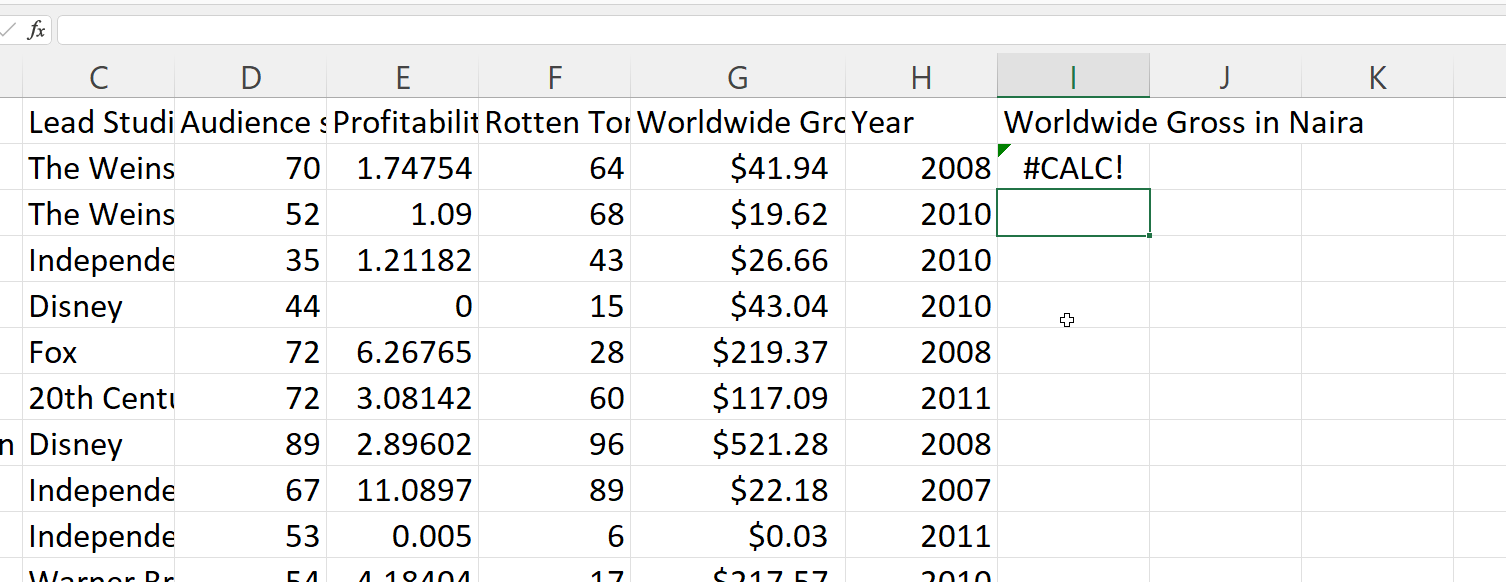
5. To make use of the newly created function, you need to copy the syntax written.
6. Go to the formula ribbon and open the name manager.
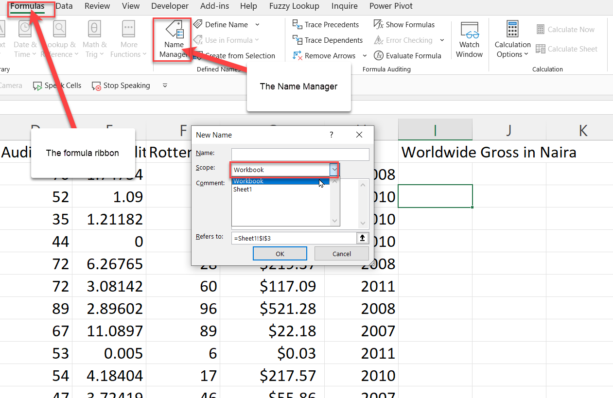
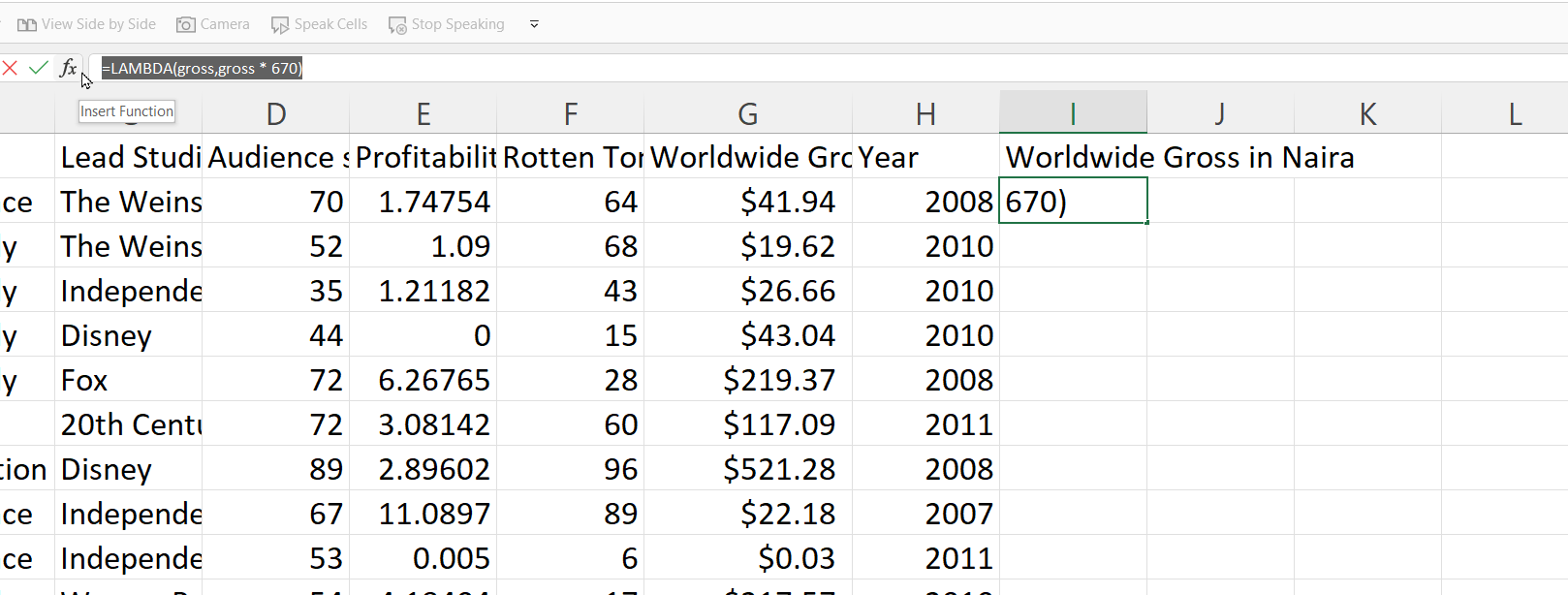
7. Define the name manger parameters:
- The name is simply what you want to call this function. I am going with NairaConvert.
- The scope should be workbook because you want to use this function in the workbook.
- The comments explains what your function does. It is acts as a documentation.
- In the refer to, you should paste the copied function syntax.
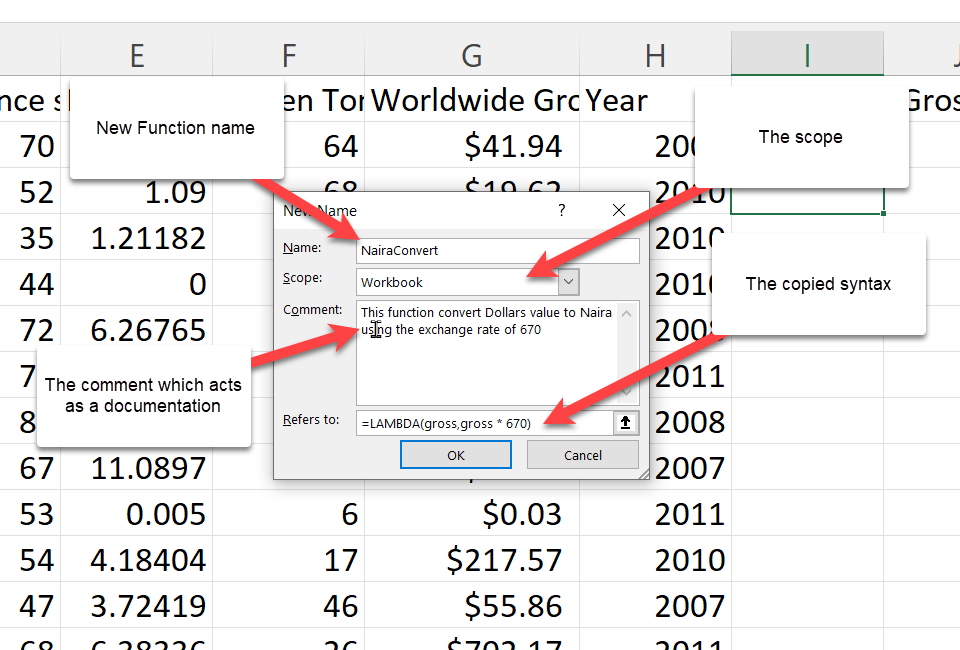
8. Press Ok.
9. To use this new function, you call it with the name you defined it as—NairaConvert—and give it the gross which is our worldwise gross on G2.
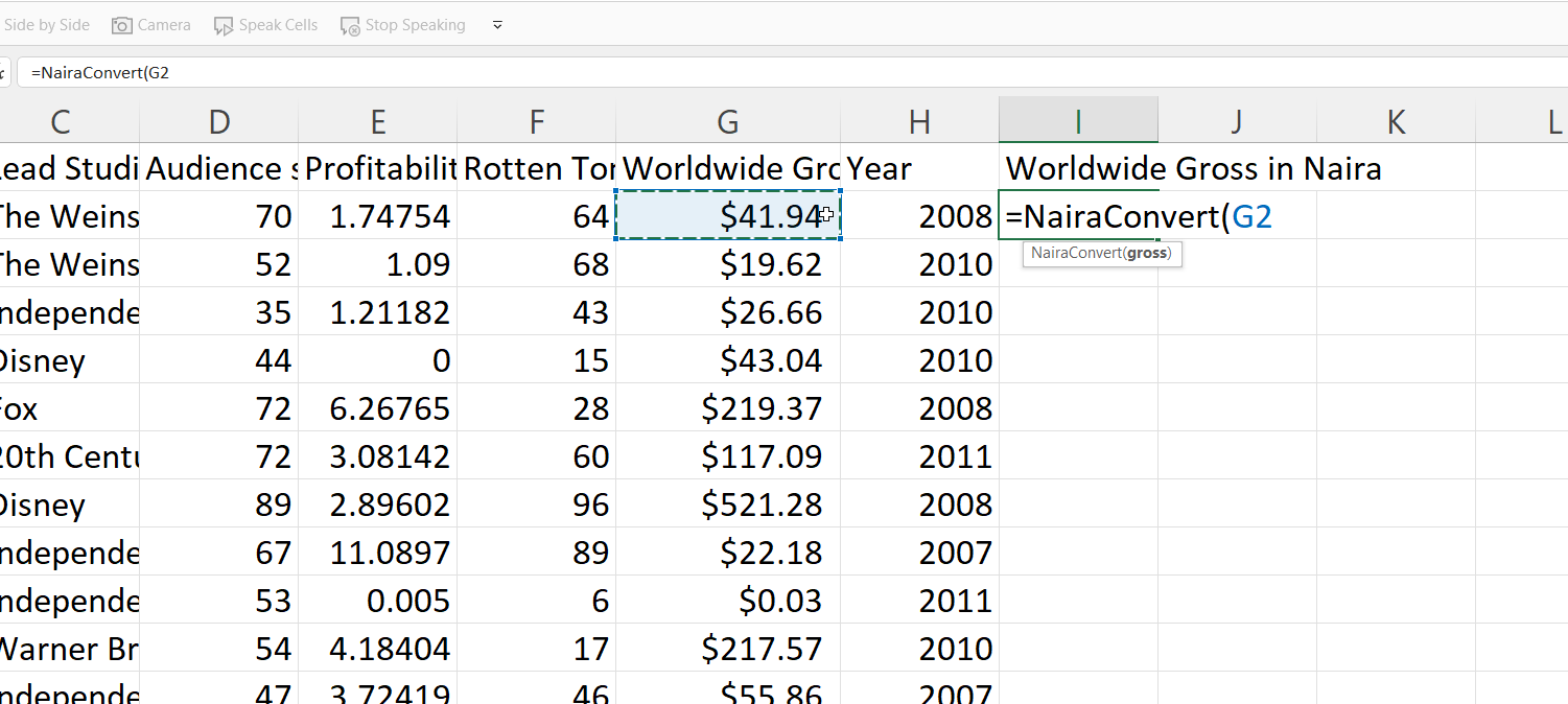
10. Close the parenthesis and press Ok
Where Can I Learn More about Excel?
There are a ton of resources for learning Microsoft Excel nowadays. So many that it is hard to figure out which ones are up-to-date and helpful.
The best thing you can do is find a helpful tutorial and follow it to completion, instead of attempting to take several at once. I would advise you to start with freeCodeCamp’s Microsoft Excel Tutorial for Beginners — Full Course, which is available on YouTube.
You should also join communities like the Microsoft Excel and Data Analysis Learning Community. However, if you’re looking for a compilation of resources, check out freeCodeCamp’s publication Excel tags.
If you enjoyed reading this article and/or have any questions and want to connect, you can find me on LinkedIn or Twitter.
Learn to code for free. freeCodeCamp’s open source curriculum has helped more than 40,000 people get jobs as developers. Get started