
Add or remove items from a drop-down list
Excel for Microsoft 365 Excel for Microsoft 365 for Mac Excel for the web Excel 2021 Excel 2021 for Mac Excel 2019 Excel 2019 for Mac Excel 2016 Excel 2016 for Mac Excel 2013 Excel 2010 Excel 2007 More…Less
After you create a drop-down list, you might want to add more items or delete items. In this article, we’ll show you how to do that depending on how the list was created.
Edit a drop-down list that’s based on an Excel Table
If you set up your list source as an Excel table, then all you need to do is add or remove items from the list, and Excel will automatically update any associated drop-downs for you.
-
To add an item, go to the end of the list and type the new item.
-
To remove an item, press Delete.
Tip: If the item you want to delete is somewhere in the middle of your list, right-click its cell, click Delete, and then click OK to shift the cells up.
-
Select the worksheet that has the named range for your drop-down list.
-
Do any of the following:
-
To add an item, go to the end of the list and type the new item.
-
To remove an item, press Delete.
Tip: If the item you want to delete is somewhere in the middle of your list, right-click its cell, click Delete, and then click OK to shift the cells up.
-
-
Go to Formulas > Name Manager.
-
In the Name Manager box, click the named range you want to update.

-
Click in the Refers to box, and then on your worksheet select all of the cells that contain the entries for your drop-down list.
-
Click Close, and then click Yes to save your changes.
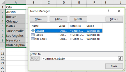
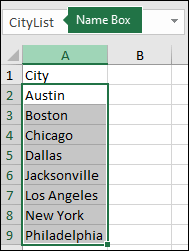
Tip: If you don’t know what a named range is named, you can select the range and look for its name in the Name Box. To locate a named range, see Find named ranges.
-
Select the worksheet that has the data for your drop-down list.
-
Do any of the following:
-
To add an item, go to the end of the list and type the new item.
-
To remove an item, click Delete.
Tip: If the item you want to delete is somewhere in the middle of your list, right-click its cell, click Delete, and then click OK to shift the cells up.
-
-
On the worksheet where you applied the drop-down list, select a cell that has the drop-down list.
-
Go to Data > Data Validation.
-
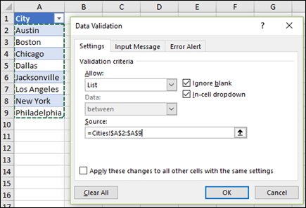
On the Settings tab, click in the Source box, and then on the worksheet that has the entries for your drop-down list, select all of the cells containing those entries. You’ll see the list range in the Source box change as you select.
-
To update all cells that have the same drop-down list applied, check the Apply these changes to all other cells with the same settings box.
-
On the worksheet where you applied the drop-down list, select a cell that has the drop-down list.
-
Go to Data > Data Validation.
-
On the Settings tab, click in the Source box, and then change your list items as needed. Each item should be separated by a comma, with no spaces in between like this: Yes,No,Maybe.
-
To update all cells that have the same drop-down list applied, check the Apply these changes to all other cells with the same settings box.
After you update a drop-down list, make sure it works the way you want. For example, check to see if the cell is wide enough to show your updated entries.
If the list of entries for your drop-down list is on another worksheet and you want to prevent users from seeing it or making changes, consider hiding and protecting that worksheet. For more information about how to protect a worksheet, see Lock cells to protect them.
If you want to delete your drop-down list, see Remove a drop-down list.
To see a video about how to work with drop-down lists, see Create and manage drop-down lists.
Edit a drop-down list that’s based on an Excel Table
If you set up your list source as an Excel table, then all you need to do is add or remove items from the list, and Excel will automatically update any associated drop-downs for you.
-
To add an item, go to the end of the list and type the new item.
-
To remove an item, press Delete.
Tip: If the item you want to delete is somewhere in the middle of your list, right-click its cell, click Delete, and then click OK to shift the cells up.
-
Select the worksheet that has the named range for your drop-down list.
-
Do any of the following:
-
To add an item, go to the end of the list and type the new item.
-
To remove an item, press Delete.
Tip: If the item you want to delete is somewhere in the middle of your list, right-click its cell, click Delete, and then click OK to shift the cells up.
-
-
Go to Formulas > Name Manager.
-
In the Name Manager box, click the named range you want to update.
-
Click in the Refers to box, and then on your worksheet select all of the cells that contain the entries for your drop-down list.
-
Click Close, and then click Yes to save your changes.
Tip: If you don’t know what a named range is named, you can select the range and look for its name in the Name Box. To locate a named range, see Find named ranges.
-
Select the worksheet that has the data for your drop-down list.
-
Do any of the following:
-
To add an item, go to the end of the list and type the new item.
-
To remove an item, click Delete.
Tip: If the item you want to delete is somewhere in the middle of your list, right-click its cell, click Delete, and then click OK to shift the cells up.
-
-
On the worksheet where you applied the drop-down list, select a cell that has the drop-down list.
-
Go to Data > Data Validation.
-
On the Settings tab, click in the Source box, and then on the worksheet that has the entries for your drop-down list, Select cell contents in Excel containing those entries. You’ll see the list range in the Source box change as you select.
-
To update all cells that have the same drop-down list applied, check the Apply these changes to all other cells with the same settings box.
-
On the worksheet where you applied the drop-down list, select a cell that has the drop-down list.
-
Go to Data > Data Validation.
-
On the Settings tab, click in the Source box, and then change your list items as needed. Each item should be separated by a comma, with no spaces in between like this: Yes,No,Maybe.
-
To update all cells that have the same drop-down list applied, check the Apply these changes to all other cells with the same settings box.
After you update a drop-down list, make sure it works the way you want. For example, check to see how to Change the column width and row height to show your updated entries.
If the list of entries for your drop-down list is on another worksheet and you want to prevent users from seeing it or making changes, consider hiding and protecting that worksheet. For more information about how to protect a worksheet, see Lock cells to protect them.
If you want to delete your drop-down list, see Remove a drop-down list.
To see a video about how to work with drop-down lists, see Create and manage drop-down lists.
In Excel for the web, you can only edit a drop-down list where the source data has been entered manually.
-
Select the cells that have the drop-down list.
-
Go to Data > Data Validation.
-
On the Settings tab, click in the Source box. Then do one of the following:
-
If the Source box contains drop-down entries separated by commas, then type new entries or remove ones you don’t need. When you’re done, each entry should be separated by a comma, with no spaces. For example: Fruits,Vegetables,Meat,Deli.
-
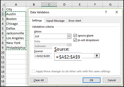
If the Source box contains a reference to a range of cells (for example, =$A$2:$A$5), click Cancel, and then add or remove entries from those cells. In this example, you’d add or remove entries in cells A2 through A5. If the list of entries ends up being longer or shorter than the original range, go back to the Settings tab and delete what’s in the Source box. Then click and drag to select the new range containing the entries.
-
If the Source box contains a named range, like Departments, then you need to change the range itself using a desktop version of Excel.
-
After you update a drop-down list, make sure it works the way you want. For example, check to see if the cell is wide enough to show your updated entries. If you want to delete your drop-down list, see Remove a drop-down list.
Need more help?
You can always ask an expert in the Excel Tech Community or get support in the Answers community.
See Also
Create a drop-down list
Apply Data Validation to cells
Video: Create and manage drop-down lists
Need more help?
Want more options?
Explore subscription benefits, browse training courses, learn how to secure your device, and more.
Communities help you ask and answer questions, give feedback, and hear from experts with rich knowledge.
|December 4, 2019||Power Query
This post will demonstrate how to insert the same few items into a list and create a new row for each item (or each combination, if multiple items). For example, let’s say we have a list of some sort … we’ll use a list of T-Shirts for this illustration. We have a few T-Shirt options that we want repeated for each T-shirt in our list. For example, each T-shirt has the same size and color options. We’d like to expand the list of T-shirts and create a new row for each combination of color and size. I’ll demonstrate how we can use Power Query to accomplish this task.
Video
Objective
Before we get to the detailed steps, let’s quickly confirm our objective.
We have a list of T-shirts, like this:

We want to expand the list so that each T-shirt gets a new row for each size option (small, medium, large) and a new row for each color option (blue, black, white, red). The resulting list needs to have a new row for each combination of size and color, like this:

In the old days, this took quite a bit of copy/paste, or perhaps a clever macro. Nowadays, it is just a couple of clicks in Power Query.
Let’s get to it.
Narrative
We’ll accomplish our objective with these steps:
- Get list into Power Query
- Create size and color columns
- Split columns into rows
First up, getting the T-Shirt list into Power Query.
Get list into Power Query
To load our list into Power Query, we select any cell in the table and use the Data > From Table/Range command.
This will load our T-Shirt table into Power Query, and we should see something like this in the Power Query Editor:

Done. Time to create the size and color columns.
Create size and color columns
Our goal in this step is to create one column for each option list. Here, we have two options (size and color), so we’ll create two columns. Each column will contain a delimited list of values for example, small, medium, large. The end game is that we will ultimately split the delimited lists into new rows. So at this point, we just need to get the delimited lists into each row.
There are several ways to create the Size and Color columns. In this example, we’ll use Custom Columns. From within Power Query select the Add Column > Custom Column command. In the resulting Custom Column dialog, we enter the new column name as Size and the formula as = “Small,Medium,Large” (no spaces around the commas) as shown below:

We hit OK and now the size values are repeated in each row:

Now, we need to create the Color column. So, again, we use the Add Column > Custom Column command, and enter the corresponding formula:

Hit OK and so far so good:

Now that we have the desired option values in new columns, it is time to split these values into rows in order to create one new row for each combination of size and color.
Split columns into rows
First, we select the column we’d like to split. In this case, we’ll start with the Size column:

We select the Transform > Text Column > Split Column > By Delimiter command. In the resulting dialog, we identify the delimiter (in our case, a comma) and we want to Split at Each occurrence of the delimiter. Then we click Advanced options to reveal the Split into Rows option:

We click OK and confirm that there is one new row for each Size:

We repeat these steps for the Color column and bam:

We are looking good, so we just click Home > Close & Load To and send the results back into an Excel table:

The results are displayed in Excel:
Now, the beautiful thing about Power Query is that next period, when we have additional T-Shirts in our products table, all we need to do is right-click the results table and hit Refresh. And, if we have any additional colors or sizes, we can simply open up the query and modify our custom column formula (by clicking the gear icon) to include them. When we Close & Load, the updated values will flow into the results table!
Conclusion
If you have any other ways to accomplish this or suggestions on how this approach can be improved, please share by posting a comment below … thanks!
Sample File: RepeatOptions.xlsx
When we need to collect data from others, they may write different things from their perspective. Still, we need to make all the related stories under one. Also, it is common that while entering the data, they make mistakes because of typo errors. For example, assume in certain cells, if we ask users to enter either “YES” or “NO,” one will enter “Y,” someone will insert “YES” like this, and we may end up getting a different kind of results. So in such cases, creating a list of values as pre-determined values allows the users only to choose from the list instead of users entering their values. Therefore, in this article, we will show you how to create a list of values in Excel.
Table of contents
- Create List in Excel
- #1 – Create a Drop-Down List in Excel
- #2 – Create List of Values from Cells
- #3 – Create List through Named Manager
- Things to Remember
- Recommended Articles
You can download this Create List Excel Template here – Create List Excel Template
#1 – Create a Drop-Down List in Excel
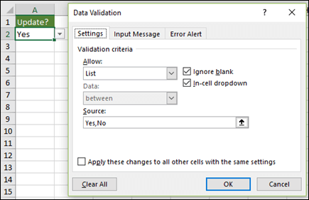
We can create a drop-down list in Excel using the “Data Validation in excelThe data validation in excel helps control the kind of input entered by a user in the worksheet.read more” tool, so as the word itself says, data will be validated even before the user decides to enter. So, all the values that need to be entered are pre-validated by creating a drop-down list in Excel. For example, assume we need to allow the user to choose only “Agree” and “Not Agree,” so we will create a list of values in the drop-down list.
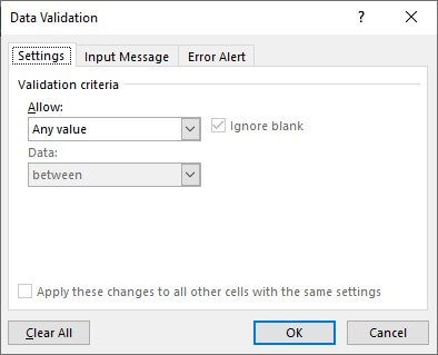
- In the Excel worksheet under the “Data” tab, we have an option called “Data Validation” from this again, choose “Data Validation.”

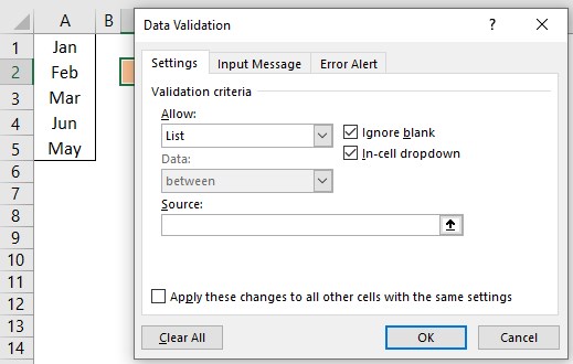
- As a result, this will open the “Data Validation” tool window.
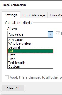
- The “Settings” tab will be shown by default, and now we need to create validation criteria. Since we are creating a list of values, choose “List” as the option from the “Allow” drop-down list.
- For this “List,” we can give a list of values to be validated in the following way, i.e., by directly entering the values in the “Source” list.

- Enter the first value as “Agree.”
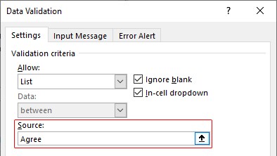
- Once the first value to be validated is entered, we need to enter “comma” (,) as the list separator before entering the next value. So, enter “comma” and enter the following values as “Not Agree.”
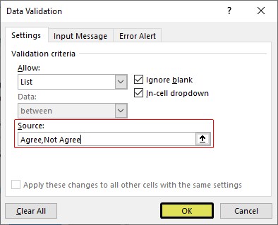
- After that, click on “Ok,” and the list of values may appear in the form of the “drop-down” list.

#2 – Create a List of Values from Cells
The above method is to get started, but imagine the scenario of creating a long list of values or your list of values changing now and then. Then, it may get difficult to return and edit the list of values manually. So, by entering values in the cell, we can easily create a list of values in Excel.
Follow the steps to create a list from cell values.
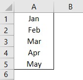
- We must first insert all the values in the cells.

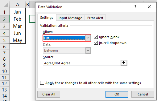
- Then, open “Data Validation” and choose the validation type as “List.”

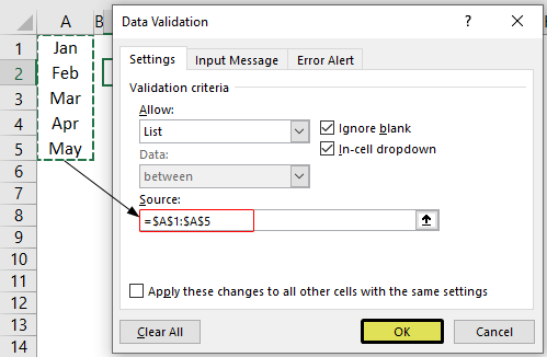
- Next, in the “Source” box, we need to place the cursor and select the list of values from the range of cells A1 to A5.

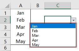
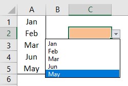
- Click on “OK,” and we will have the list ready in cell C2.

So values to this list are supplied from the range of cells A1 to A5. Any changes in these referenced cells will also impact the drop-down list.
For example, in cell A4, we have a value as “Apr,” but now we will change that to “Jun” and see what happens in the drop-down list.
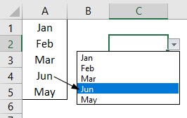
Now, look at the result of the drop-down list. Instead of “Apr,” we see “Jun” because we had given the list source as cell range, not manual entries.
#3 – Create List through Named Manager
There is another way to create a list of values, i.e., through named ranges in excelName range in Excel is a name given to a range for the future reference. To name a range, first select the range of data and then insert a table to the range, then put a name to the range from the name box on the left-hand side of the window.read more.
- We have values from A1 to A5 in the above example, naming this range “Months.”

- Now, select the cell where we need to create a list and open the drop-down list.
- Now place the cursor in the “Source” box and press the F3 key to an open list of named ranges.
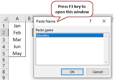
- As we can see above, we have a list of names, choose the name “Months” and click on “OK” to get the name to the “Source” box.
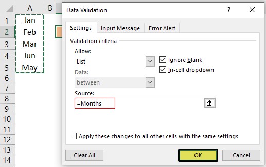
- Click on “OK,” and the drop-down list is ready.
Things to Remember
- The shortcut key to open data validation is “ALT + A + V + V.“
- We must always create a list of values in the cells so that it may impact the drop-down list if any change happens in the referenced cells.
Recommended Articles
This article has been a guide to Excel Create List. Here, we learn how to create a list of values in Excel also, create a simple drop-down method and make a list through name manager along with examples and downloadable Excel templates. You may learn more about Excel from the following articles: –
- Custom List in Excel
- Drop Down List in Excel
- Compare Two Lists in Excel
- How to Randomize List in Excel?
Excel has some useful features that allow you to save time and be a lot more productive in your day-to-day work.
One such useful (and less-known) feature in the Custom Lists in Excel.
Now, before I get to how to create and use custom lists, let me first explain what’s so great about it.
Suppose you have to enter numbers the month names from Jan to Dec in a column. How would you do it? And no, doing it manually is not an option.
One of the fastest ways would be to have January in a cell, February in an adjacent cell and then use the fill handle to drag and let Excel automatically fill in the rest. Excel is smart enough to realize that you want to fill the next month in each cell in which you drag the fill handle.
Month names are quite generic and therefore it’s available by default in Excel.
But what if you have a list of department names (or employee names or product names), and you want to do the same. Instead of manually entering these or copy-paste these, you want these to appear magically when you use the fill handle (just like month names).
You can do that too…
… by using Custom Lists in Excel
In this tutorial, I will show you how to create your own custom lists in Excel and how to use these to save time.
How to Create Custom Lists in Excel
By default, Excel already has some pre-fed custom lists that you can use to save time.
For example, if you enter ‘Mon’ in one cell ‘Tue’ in an adjacent cell, you can use the fill handle to fill the rest of the days. In case you extend the selection, keep on dragging and it will repeat and give you the day’s name again.

Below are the custom lists that are already in-built in Excel. As you can see, these are mostly days and month names as these are fixed and will not change.

Now, suppose you want to create a list of departments that you often need in Excel, you can create a custom list for it. This way, the next time you need to get all the departments name in one place, you don’t need to rummage through old files. All you need to do is type the first two in the list and drag.

Below are the steps to create your own Custom List in Excel:
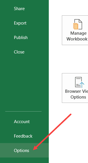
- Click the File tab

- Click on Options. This will open the ‘Excel Options‘ dialog box

- Click on the Advanced option in the left-pane

- In the General option, click on the ‘Edit Custom Lists’ button (you may have to scroll down to get to this option)

- In the Custom Lists dialog box, import the list by selecting the range of cells that have the list. Alternatively, you can also enter the name manually in the List Entries box (separated by comma or each name in a new line)

- Click on Add


As soon as you click on Add, you would notice that your list now becomes a part of the Custom Lists.

In case you have a large list that you want to add to Excel, you can also use the Import option in the dialog box.
Pro tip: You can also create a named range and use that named range to create the custom list. To do this, enter the name of the named range in the ‘Import list from cells’ field and click OK. The benefit of this is that you can change or expand the named range and it will automatically get adjusted as the custom list
Now that you have the list in Excel backend, you can use it just like you use numbers or month names with Autofill (as shown below).

While it’s great to be able to quickly get these custom lits names in Excel by doing a simple drag and drop, there is something even more awesome that you can do with custom lists (that’s what the next section is about).
Create Your Own Sorting Criteria Using Custom Lists
One great thing about custom lists is that you can use it to create your own sorting criteria. For example, suppose you have a dataset as shown below and you want to sort this based on High, Medium, and Low.

You can’t do this!
If you sort alphabetically, it would screw the alphabetical order (it will give you High, Low, and Medium and not High, Medium, and Low).
This is where Custom Lists really shine.
You can create your own list of items and then use these to sort the data. This way, you will get all the High values together at the top followed by the medium and low values.
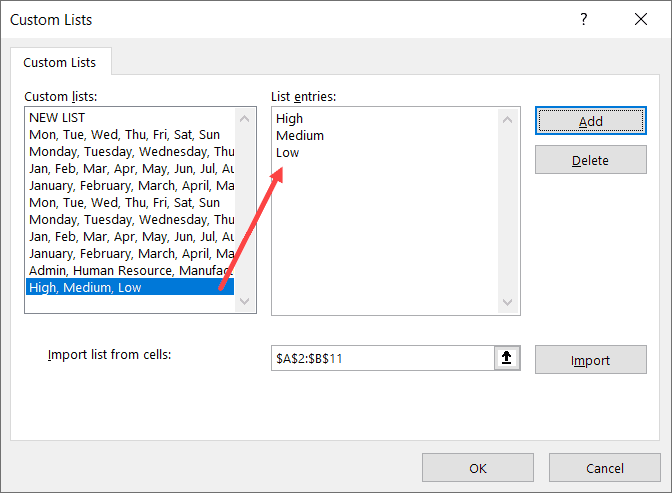
The first step is to create a custom list (High, Medium, Low) using the steps shown in the previous section (‘How to Create Custom Lists in Excel‘).
Once you have the custom list created, you can use the below steps to sort based on it:
- Select the entire dataset (including the headers)
- Click the Data tab

- In the Sort and Filter group, click on the Sort icon. This will open the Sort dialog box

- In the Sort dialog box, make the following selections:
- Sort by Column: Priority
- Sort On: Cell Values
- Order: Custom Lists. When the dialog box opens, select the sorting criteria you want to use and then click on OK.

- Click OK


The above steps would instantly sort the data using the list you created and used as criteria while sorting (High, Medium, Low in this example).

Note that you don’t necessarily need to create the custom list first to use it in sorting. You can use the above steps and in Step 4 when the dialog box opens, you can create a list right there in that dialog box.
Some Examples Where you can Use Custom Lists
Below are some of the cases where creating and using custom lists can save you time:
- If you have a list that you need to enter manually (or copy-paste from some other source), you can create a custom list and use that instead. For example, this could be department names in your organization, or product names or regions/countries.
- If you’re a teacher, you can create a list of your student names. That way, when you are grading them the next time, you don’t need to worry about entering the student names manually or copy-pasting it from some other sheet. This also ensures that there are fewer chances of errors.
- When you need to sort data based on criteria that are not in-built in Excel. As covered in the previous section, you can use your own sorting criteria by making a custom list in Excel.
So this is all that you need to know about Creating Custom Lists in Excel.
I hope you found this useful.
You may also like the following Excel tutorials:
- How to Sort by the Last Name in Excel
- How to SORT in Excel (by Rows, Columns, Colors, Dates, & Numbers)
- How to Sort By Color in Excel
- How to Sort Worksheets in Excel
- Automatically Sort Data in Alphabetical Order using Formula
One of the best ways to learn new techniques in Excel is to see them in action. This post demonstrates how to add some fun and useful features to simple to do lists including drop-down lists, check boxes, progress bars, and more. The images show Excel 2016, but instructions are similar for Excel 2010 and Excel 2013.
This Page (contents):
- Simple Drop-Down Lists via Data Validation
- Conditional Formats for the Priority Column
- Conditional Formats for Numeric Priority
- Checkboxes using Form Fields
- Checkboxes via Data Validation
- Progress Bar for % Completed
- Gray-Out Tasks When They are Complete
- Highlighting Overdue Dates
- Autofilter and Sorting
- Create a Gantt Chart
- Drop-Down with Current Date
1. Simple Drop-Down Lists via Data Validation
Many task lists include a Priority or Status column, such as the Homework To Do List shown below. It’s very handy to use an Excel drop down list for columns like these.
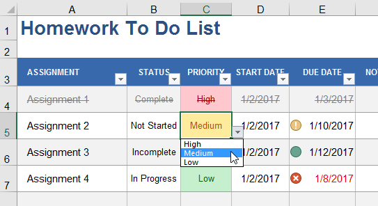
To create a simple drop-down list, follow these steps:
- Select the cells you want to edit
- Go to Data > Data Validation
- Choose «List» in the Allow field
- In the Source field enter a comma-delimited list such as High,Medium,Low
2. Conditional Formats for the Priority Column
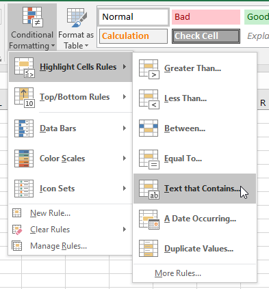
In the example above you will see that the values in the Priority column have been highlighted differently. This can be done automatically and is a great way to easily identify your high-priority tasks. Follow these steps to create the type of formats shown in the example above.
- Select the cells in the Priority column
- Go to Home > Conditional Formatting > Text That Contains
- Enter the word high and choose the «Light Red Fill with Dark Red Text» option
The image below shows how to get to the correct option from the Home tab.
3. Conditional Formats for Numeric Priority
If you want to use a numeric priority like 0-4, then you can use Icon Sets to display images instead of (or in addition to) the numeric value. You can see this demonstrated in the Simple Task Tracker below.
![]()
- Select the cells in the Priority column
- Create a drop-down list with the options 4,3,2,1
- Go to Home > Conditional Formatting > Icon Sets > More Rules
- The image below shows you how to modify the settings for this rule.
![]()
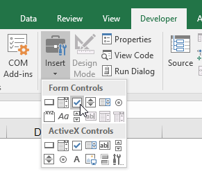
4. Checkboxes using Form Fields
I don’t like this method. If you like to sort and delete and insert rows, form fields get all messed up. They may be nice for a spreadsheet layout that is not meant to be modified, but so far I haven’t found a to do list that I haven’t wanted to modify frequently.
The form field checkbox is found in the Developer tab shown in the image below. If you don’t see the Developer tab, go to File > Excel Options > Customize Ribbon and find and check the Developer tab.
5. Checkboxes via Data Validation
I wish Microsoft would add an in-cell checkbox feature (Apple’s Numbers software does it), but until they do that we have to come up with clever alternatives.
One method I like is using a data validation drop-down list because it works pretty well in Excel on touch-enabled devices, and it is also compatible with most versions of Excel and OpenOffice and Google Sheets.
The simplest checkbox to make using a drop-down list is probably just a list with a single character (x), or you could use a special character like the square root sign (√) that looks like a check mark in some fonts. In the example below, I’ve used this technique plus a small square ascii character (□,√).
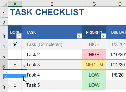
Another approach that I really like is to use custom Icon Sets via Conditional Formatting. This isn’t as compatible with other spreadsheet programs (like Google Sheets) but it looks good. The simple Task Tracker Template shows an example of this:
![]()
- Select the cells you want to use for the check boxes
- Create a drop-down list with the options 1,0,-1
- Go to Home > Conditional Formatting > Icon Sets and select any set you like
- With those cells still selected, go to Home > Conditional Formatting > Manage Rules and find the rule you just created and edit it to create a custom icon set with the setting shown in the following image.
![]()
6. Progress Bar for % Completed
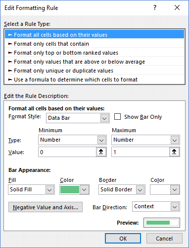
In some of the examples above, you’ve already seen progress bars in the «% Complete» column. Now you’ll learn how to do it. Conditional formatting comes in handy yet again:
- Select the cells in the % Complete column
- Go to Home > Conditional Formatting > Data Bars > More Rules
- Modify the bar based on the settings shown in the image below
Want a Progress Bar in Google Sheets? No problem. In cell A1 enter the % Complete and then in the cell to the right of it you can use the formula =REPT(«█»,ROUND(A1*10,0)). You can change the color of the bar by just changing the font color. That’s a pretty old trick for Excel users, but it’s something that will work in Google Sheets, too.
Progress Bar via SPARKLINE in Google Sheets
The new SPARKLINE function allows you to create a progress bar in Google Sheets very easily. Enter a percent complete in cell A1 and the following SPARKLINE function for the bar chart in cell A2.
A1=87.2%
A2=SPARKLINE(A1,{"charttype","bar";"color1","blue";"max",1;"min",0})
See the Simple Gantt Chart (Google Sheets version) for an example of how the SPARKLINE function can be used for progress bars.
For more ways to modify the color and look of the in-cell progress bar, see the SPARKLINE function documentation.
7. Gray-Out Tasks When They are Complete
If you like the effect of seeing your completed tasks crossed out or grayed out or both, you can do that fairly easily using conditional formatting.
In the example below, the first rule is applied when column A is equal to the special square root character. The placement of the dollar sign in the $A4 reference is very important in this formula because we want all the columns in the table to reference column A.
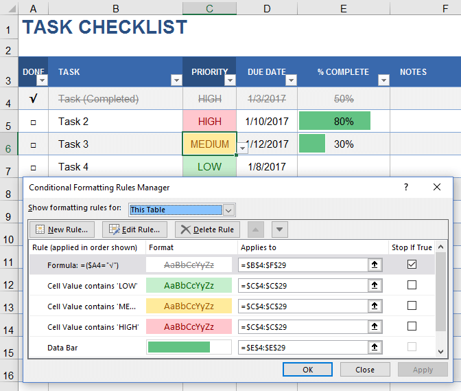
Also note that the first rule has the «Stop if True» box checked. That is why you don’t see the priority cell highlighted red or the % Complete showing a green bar in the example. When the task is marked as complete, I don’t want to be distracted by formatting that no longer matters to me. So I’m using the rule order to prevent the following rules from being applied if the task has been marked as done.
8. Highlighting Overdue Dates
When you have a Due Date, you may want to highlight the date when it is overdue. You can do that with a simple conditional formatting rule shown in the example below.
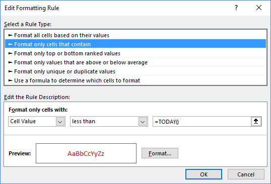
You can see an example of this in the Homework To Do List shown at the very top of this article.
9. Autofilter and Sorting
The little arrows that show up in the header of an Excel table or list are a result of turning on the Filter Button feature. If you don’t see the little arrows in the header row already, select a cell in your table (or the entire table) and go to the Data tab and click on the Filter button.
10. Create a Gantt Chart
Although a Gantt chart is a great visualization and management tool for projects, creating one from scratch is not nearly as simple as the other ideas shared in this article. The two most common ways to create a Gantt chart in Excel are (1) using a stacked bar graph chart object and (2) using conditional formatting. Visit my Task List Templates page to find an example that uses a chart object and try the free Gantt Chart Template to see the conditional formatting technique in action.
11. Drop-Down with Current Date
Update 10/9/2018 — I recently created a new wedding checklist where a user requested the ability to enter either a checkmark or the current date. To do this with data validation, create a list somewhere in the worksheet with the first cell containing a check mark unicode character ✔ and the next cell containing the formula =TODAY().
Then, use data validation to create a drop-down list referencing those two cells. This will allow you to select either a checkmark or the current date as shown in the image below.
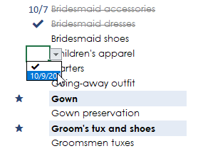
To avoid having Excel show warnings when cells contain older dates, make sure to turn off the warnings and errors when setting up the data validation.