
There may be instances where you need to add the same text to all cells in a column. You might need to add a particular title before names in a list, or a particular symbol at the end of the text in every cell.
The good thing is you don’t need to do this manually.
Excel provides some really simple ways in which you can add text to the beginning and/ or end of the text in a range of cells.
In this tutorial we will see 4 ways to do this:
- Using the ampersand operator (&)
- Using the CONCATENATE function
- Using the Flash Fill feature
- Using VBA
So let’s get started!
Method 1: Using the ampersand Operator
An ampersand (&) can be used to easily combine text strings in Excel. Let’s see how you use it to add text at the beginning or end or both in Excel.
Using the ampersand Operator to Add Text to the Beginning of all Cells
The ampersand (&) is an operator that is mainly used to join several text strings into one.
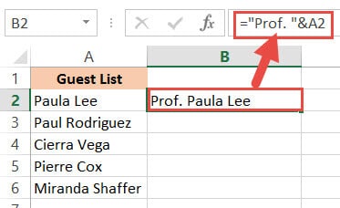
Here’s how you can use it to add text to the beginning of all cells in a range. Let us assume you have the following list of names and want to add the title “Prof.” before every name:

Below are the steps to add a text before a text string in Excel:
- Click on the first cell of the column where you want the converted names to appear (B2).
- Type equal sign (=), followed by the text “Prof. “, followed by an ampersand (&).
- Select the cell containing the first name (A2).
- Press the Return Key.
- You will notice that the title “Prof.” is added before the first name in the list.

- It’s now time to copy this formula to the rest of the cells in the column. Simply double click the fill handle (located at the bottom right of cell B2). Alternatively, you can drag down the fill handle to achieve the same effect.
That’s it, all your cells in column B should now contain the title “Prof.” preceding each name.

Using the ampersand Operator to Add Text to the End of all Cells
Now let us see how to add some text to the end of every name in the dataset. Let us say you want to add the text “(MD)” at the end of every name. In that case, here are the steps you need to follow:
- Click on the first cell of the column where you want the converted names to appear (C2 in our case).
- Type equal sign (=)
- Select the cell containing the first name (B2 in our case).
- Next, insert an ampersand (&), followed by the text “ (MD)”.
- Press the Return Key.
- You will notice that the text “(MD).” added after the first name in the list.

- It’s now time to copy this formula to the rest of the cells in the column. Simply double click the fill handle (located at the bottom right of cell C2). Alternatively, you can drag down the fill handle to achieve the same effect.

All your cells in column C should now contain the text “(MD”) at the end of each name.

Method 2: Using the CONCATENATE Function
CONCATENATE is an Excel function that you can use to add text at the beginning and end of the text string.
Let’s see how to use CONCATENATE to do this.
Using CONCATENATE to Add Text to the Beginning of all Cells
The CONCATENATE() function provides the same functionality as the ampersand (&) operator. The only difference is in the way both are used.
The general syntax for the CONCATENATE function is:
=CONCATENATE(text1, [text2], …)
Where text1, text2, etc. are substrings that you want to combine together.
Let’s apply the CONCATENATE function to the same dataset as above:
- Click on the first cell of the column where you want the converted names to appear (B2).
- Type equal sign (=).
- Enter the function CONCATENATE, followed by an opening bracket (.
- Type the title “Prof. ” in double-quotes, followed by a comma (,).
- Select the cell containing the first name (A2)
- Place a closing bracket. In our example, your formula should now be: =CONCATENATE(“Prof. “,A2).
- Press the Return Key.
- You will notice that the title “Prof.” is added before the first name on the list.

- It’s now time to copy this formula to the rest of the cells in the column. Simply double click the fill handle (located at the bottom right of cell B2). Alternatively, you can drag down the fill handle to achieve the same effect.

That’s it, all your cells in column B should now contain the title “Prof.” preceding each name.

Using CONCATENATE to Add Text to the End of all Cells
Now let us see how to add some text to the end of every name in the dataset. Let us say you want to add the text “(MD)” at the end of every name. In that case, here are the steps you need to follow:
- Click on the first cell of the column where you want the converted names to appear (C2 in our example).
- Type equal sign (=).
- Enter the function CONCATENATE, followed by an opening bracket (.
- Select the cell containing the first name (B2 in our example).
- Next, insert a comma, followed by the text “ (MD)”.
- Place a closing bracket. In our example, your formula should now be: =CONCATENATE(B2,” (MD)”).
- Press the Return Key.
- You will notice that the text “(MD).” added after the first name in the list.

- It’s now time to copy this formula to the rest of the cells in the column. Simply double click the fill handle (located at the bottom right of cell C2).

All your cells in column C should now contain the text “(MD”) at the end of each name.

Notice that since you’re using a formula, your column C depends on columns A and B. So if you make any changes to the original values in column A, they get reflected in column C.
If you decide to only retain the converted names and delete columns A and B, you will get an error, as shown below:

To make sure that this does not happen, it’s best to first convert the formula results to permanent values copying them and pasting them as values in the same column (Right-click and select Paste Options->Values from the Popup menu).

Now you can go ahead and delete columns A and B if you need to.
Also read: How to Remove First Character in Excel?
Method 3: Using the Flash Fill Feature
Flash fill is a relatively new feature that looks at the pattern of what you are trying to achieve and then does it for all the cells in a column.
You can also use Flash fill to so text manipulation as we will see in the following examples.
Using Flash Fill to Add Text to the Beginning of all Cells
The Excel flash fill feature is like a magical button. It is available if you’re on any Excel version from 2013 onwards.
The feature takes advantage of Excel’s pattern recognition capabilities. It basically recognizes a pattern in your data and automatically fills in the other cells of the column with the same pattern for you.
Here’s how you can use Flash Fill to add text to the beginning of all cells in a column:
- Click on the first cell of the column where you want the converted names to appear (B2).
- Manually type in the text Prof. , followed by the first name of your list.

- Press the Return Key.
- Click on cell B2 again.
- Under the Data tab, click on the Flash Fill button (in the ‘Data Tools’ group). Alternatively, you can just press CTRL+E on your keyboard (Command+E if you’re on a Mac).


This will copy the same pattern to the rest of the cells in the column… in a flash!

Using Flash Fill to Add Text to the End of all Cells in a Column
If you want to add the text “ (MD)” to the end of the names, follow the same steps:
- Click on the first cell of the column where you want the converted names to appear (C2).
- Manually type in or copy the text from column B2 into C2.
- Add the text “(MD)” after that.

- Under the Data tab, click on the Flash Fill or press CTRL+E on your keyboard (Command+E if you’re on a Mac).

That’s all, you get every cell filled in with the same pattern!

We especially like this method because it is simple, quick, and easy. Moreover, since it’s formula-free, the results do not depend on the original columns.
So they remain unchanged even if you delete rows A and B!

Method 4: Using VBA Code
And of course, if you’re comfortable with VBA, you can also add text before or after a text string using it.
Using VBA to Add Text to the Beginning of all Cells in a Column
If coding with VBA does not intimidate you then this method can help get your work done quickly too.
Here’s the code we will be using to add the title “Prof. “ to the beginning of all cells in a range. You can select and copy it:
Sub add_text_to_beginning()
Dim rng As Range
Dim cell As Range
Set rng = Application.Selection
For Each cell In rng
cell.Offset(0, 1).Value = "Prof. " & cell.Value
Next cell
End Sub
Follow these steps to use the above code:
- From the Developer Menu Ribbon, select Visual Basic.
- Once your VBA window opens, Click Insert->Module. Now you can start coding. Type or copy-paste the above lines of code into the module window. Your code is now ready to run.
- Select the range of cells containing the text you want to convert. Make sure the column next to it is blank because this is where the code will display the results.
- Navigate to Developer->Macros-> add_text_to_beginning->Run.
You will now see the converted text next to your selected range of cells.
Note: You can change the text in line 6 from “Prof. ” to whatever text you need to add to the beginning of all cells.
Using VBA to Add Text to the End of all Cells in a Column
Now, what if you want to add text to the end of all the cells, instead of the beginning? This only involves making a tweak to line 6 of the above code. So if you want to add the text “ (MD)” to the end of all cells, change line 6 to:
cell.Offset(0, 1).Value = cell.Value & “ (MD)”
So your full code should now be:
Sub add_text_to_end()
Dim rng As Range
Dim cell As Range
Set rng = Application.Selection
For Each cell In rng
cell.Offset(0, 1).Value = cell.Value & " (MD)"
Next cell
End Sub
Here’s the final result:
You can now delete the first two columns if you need to. Do remember to keep a backup of your sheet, because the results of VBA code are usually irreversible.
Note: You can change the text in line 6 from “ (MD)” to whatever text you need to add to the end of all cells in the range.
In this tutorial, we showed you four ways in which you can add text to the beginning and/ or end of all cells in a range.
There are plenty of other methods that you can find online too, and all of them work just as well as the ones shown here.
You may feel free to choose whatever method suits you, your requirement, and your version of Excel. In the end, what matters is getting what you need to be done quickly and effectively.
Other Excel tutorials you may like:
- How to Remove Text after a Specific Character in Excel
- How to Reverse a Text String in Excel
- How to Count How Many Times a Word Appears in Excel
- How to Remove Commas in Excel (from Numbers or Text String)
- How to Remove a Specific Character from a String in Excel
- How to Change Uppercase to Lowercase in Excel
- How to Separate Address in Excel?
- How to Concatenate with Line Breaks in Excel?
- How to Separate Names in Excel
This is addition to @Edward-Leno ‘s answer for more detail/explanation and cases where the text cells are formulas instead of values, and you want to retain the original formula.
Suppose your cells look like this (formulas)
=»email» & «@» & «address.com»
=A1 & «@» & C1
instead of this (values)
email@address.com
If «email» and «address.com» were some cells like A1 is the email and C1 is the address.com part, then you’d have something like =A1&»@»&C1 which would be important to retain since A1 and C1 might not be constants and can change, so the comma-concatenated values would change, like if C1 is «gmail.com», «yahoo.com», or something else based on its formula.
Values method: The following steps will successfully append text but only keep the value using a scratch column (this works for rows, too, but for simplicity, the directions are for columns)
- Assume column A is your data.
- In scratch column B, start anywhere like the top of column B such as at B1 and put this formula:
=A1&»,»
Essentially, the «&» is the concatenation operator, combining two strings together (numbers are converted to strings). The «,» can be adjusted to «, » if you want a space after the comma.
-
Copy the cell B1 and copy it down to all other cells in column B, either by clicking at the bottom right of cell B1 and dragging down, or copying with «Ctrl+C» or right-click > «Copy».
-
Paste B1 to all cells in column B with «Ctrl+V» or right-click > «Paste Options:» > «Paste». You should see the data looking like you intended.
-
Copy all cells in column B and paste them to where you want via right-click > «Paste Options:» > «Values». We select values so it doesn’t mess up any formatting or conditional formatting
Formula retention method: The following steps will successfully retain the original formula. The process is similar to the values method, and only step 2, the formula used to concatenate the comma, changes.
- Assume column A is your data.
- In scratch column B, start anywhere like the top of column B such as at B1 and put this formula:
=FORMULATEXT(A1)&»,»
FORMULATEXT() grabs the formula of the cell as opposed to the value of it, so a simple example would be that it grabs =2+2 instead of 4, or =A1 & «@» & C1 where A1 is «Bob» and C1 is «gmail.com» instead of Bob@gmail.com.
Note: This formula only works for Excel versions 2013 and greater. For alternative equivalent solutions for Excel 2010 and older, see this superuser answer: https://superuser.com/a/894441/495155
-
Copy the cell B1 and copy it down to all other cells in column B, either by clicking at the bottom right of cell B1 and dragging down, or copying with «Ctrl+C» or right-click > «Copy».
-
Paste B1 to all cells in column B with «Ctrl+V» or right-click > «Paste Options:» > «Paste». You should see the data looking like you intended.
-
Copy all cells in column B and paste them to where you want via right-click > «Paste Options:» > «Values». We select values so it doesn’t mess up any formatting or conditional formatting
Содержание
- Bulk Insert Text: How to Add Text to Many Existing Excel Cells at Once
- Method 1: The fastest way to bulk insert text
- Method 2: Use a string formula to combine two text parts
- Method 3: Try a workaround to insert text with the Find & Replace function
- Method 4: Bulk insert text with a VBA macro
- How to add text or character to every cell in Excel
- Excel formulas to add text/character to cell
- Concatenation operator
- CONCATENATE function
- CONCAT function
- How to add text to the beginning of cells
- How to add text to the end of cells in Excel
- Add characters to beginning and end of a string
- Combine text from two or more cells
- How to add special character to cell in Excel
- How to add text to formula in Excel
- How to insert text after Nth character
- How to add text before/after a specific character
- Add text after specific character
- Insert text before specific character
- How to add space between text in Excel cell
- How to add the same text to existing cells with VBA
- Prepend text to beginning
- Append text to end
- Add text or character to multiple cells with Ultimate Suite
Bulk Insert Text: How to Add Text to Many Existing Excel Cells at Once

You have a couple (or many) cells with text in it. Now, you want to insert more text to them. Either at the beginning, in the middle or at the end. Here is how to easily do that!
Method 1: The fastest way to bulk insert text
Because it is the fastest and most convenient way, we go with this method first.
 Use Professor Excel Tools to easily insert text – and select from further options (subscript, superscript or the position of where to insert the text).
- Select all the cell in which you want to insert text.
- Click on “Insert Text” on the Professor Excel ribbon.
- Type your text and select further options (for example, you can specify the position (add the text in the beginning of the existing text, at the end or at a character position). Also, choose if you want o insert it as normal text, subscript or superscript.
- Click on Insert.

This function is included in our Excel Add-In ‘Professor Excel Tools’
(No sign-up, download starts directly)
More than 35,000 users can’t be wrong.
Method 2: Use a string formula to combine two text parts
The second method is based on formulas. You can combine two text strings with the & sign (actually, there are four different ways to concatenate text, but using the & sign is usually the fastest).
So, let’s see how it works:
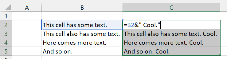 Concatenate the two text parts with the & sign.
In this example, you have existing in cells B2 to B5. You want to add the word “Cool.” to it. So, the formula in cell C2 is:
Please note that I have added a space before the word cool (on purpose…). The reason is that between the previous full stops and the word cool should have a space.
You can now copy the new cell (range C2 to C5). Paste it using paste special on top of the existing cells as values if you want to fully replace the original text cells.
Method 3: Try a workaround to insert text with the Find & Replace function
Admittedly, this method is a little bit trial and error. If it works depends on your existing cells. The main idea is to replace text from the original cells with new text.
Let’s go back to our original example. You again want to add the word “Cool.” to your existing cells:
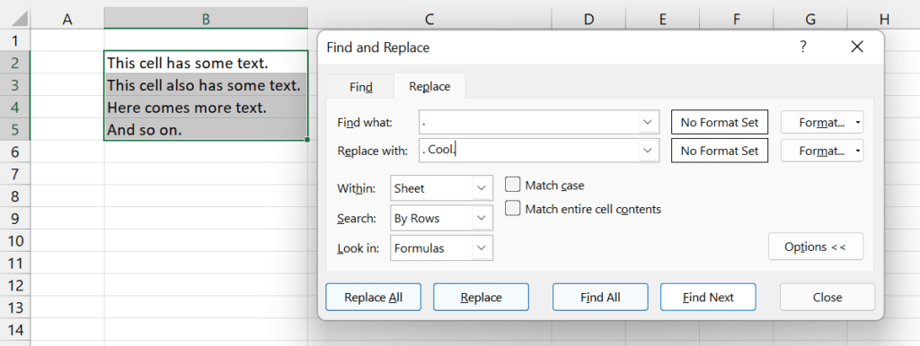 Insert text with the Find and Replace function.
In this case, we are lucky that all existing cells end with a full stop. We can use this to replace it the following way:
- Select all original cells.
- Press Ctrl + H on the keyboard so that the Find and Replace window opens.
- As “Find what:”, enter “.”
- Because we still want to keep the full stop, we also use this in the “Replace with:” field: “. Cool.”
- Click on Replace All.
If the result is not as expected, you can simply undo the replace process (press Ctrl + Z on the keyboard).
Method 4: Bulk insert text with a VBA macro
If you feel comfortable to use a short VBA macro, you can copy and paste the following code into a new VBA module. Please refer to this article for help.
Replace the word ” Cool.” with your text to add at the end. Also, you can set a text to insert in the beginning. Then, place the cursor within these lines of code and press F5 on the keyboard.
Henrik Schiffner is a freelance business consultant and software developer. He lives and works in Hamburg, Germany. Besides being an Excel enthusiast he loves photography and sports.
Источник
How to add text or character to every cell in Excel
 by Svetlana Cheusheva, updated on March 10, 2023
Wondering how to add text to an existing cell in Excel? In this article, you will learn a few really simple ways to insert characters in any position in a cell.
When working with text data in Excel, you may sometimes need to add the same text to existing cells to make things clearer. For example, you might want to put some prefix at the beginning of each cell, insert a special symbol at the end, or place certain text before a formula.
I guess everyone knows how to do this manually. This tutorial will teach you how to quickly add strings to multiple cells using formulas and automate the work with VBA or a special Add Text tool.
Excel formulas to add text/character to cell
To add a specific character or text to an Excel cell, simply concatenate a string and a cell reference by using one of the following methods.
Concatenation operator
The easiest way to add a text string to a cell is to use an ampersand character (&), which is the concatenation operator in Excel.
This works in all versions of Excel 2007 — Excel 365.
CONCATENATE function
The same result can be achieved with the help of the CONCATENATE function:
The function is available in Excel for Microsoft 365, Excel 2019 — 2007.
CONCAT function
To add text to cells in Excel 365, Excel 2019, and Excel Online, you can use the CONCAT function, which is a modern replacement of CONCATENATE:
Note. Please pay attention that, in all formulas, text should be enclosed in quotation marks.
These are the general approaches, and the below examples show how to apply them in practice.
How to add text to the beginning of cells
To add certain text or character to the beginning of a cell, here’s what you need to do:
- In the cell where you want to output the result, type the equals sign (=).
- Type the desired text inside the quotation marks.
- Type an ampersand symbol (&).
- Select the cell to which the text shall be added, and press Enter .
Alternatively, you can supply your text string and cell reference as input parameters to the CONCATENATE or CONCAT function.
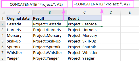
For example, to prepend the text «Project:» to a project name in A2, any of the below formulas will work.
In all Excel versions:
In Excel 365 and Excel 2019:
Enter the formula in B2, drag it down the column, and you will have the same text inserted in all cells.
Tip. The above formulas join two strings without spaces. To separate values with a whitespace, type a space character at the end of the prepended text (e.g. «Project: «).
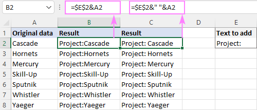
For convenience, you can input the target text in a predefined cell (E2) and add two text cells together:
Please notice that the address of the cell containing the prepended text is locked with the $ sign, so that it won’t shift when copying the formula down.
With this approach, you can easily change the added text in one place, without having to update every formula.
How to add text to the end of cells in Excel
To append text or specific character to an existing cell, make use of the concatenation method again. The difference is in the order of the concatenated values: a cell reference is followed by a text string.
For instance, to add the string «-US» to the end of cell A2, these are the formulas to use:
Alternatively, you can enter the text in some cell, and then join two cells with text together:
Please remember to use an absolute reference for the appended text ($D$2) for the formula to copy correctly across the column.

Add characters to beginning and end of a string
Knowing how to prepend and append text to an existing cell, there is nothing that would prevent you from using both techniques within one formula.
As an example, let’s add the string «Project:» to the beginning and «-US» to the end of the existing text in A2.
=CONCATENATE(«Project:», A2, «-US»)
=CONCAT(«Project:», A2, «-US»)
With the strings input in separate cells, this works equally well:

Combine text from two or more cells
To place values from multiple cells into one cell, concatenate the original cells by using the already familiar techniques: an ampersand symbol, CONCATENATE or CONCAT function.
For example, to combine values from columns A and B using a comma and a space («, «) for the delimiter, enter one of the below formulas in B2, and then drag it down the column.
Add text from two cells with an ampersand:
Combine text from two cells with CONCAT or CONCATENATE:
When adding text from two columns, be sure to use relative cell references (like A2), so they adjust correctly for each row where the formula is copied.

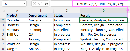
To combine text from multiple cells in Excel 365 and Excel 2019, you can leverage the TEXTJOIN function. Its syntax provides for a delimiter (the first argument), which makes the formular more compact and easier to manage.
For example, to add strings from three columns (A, B and C), separating the values with a comma and a space, the formula is:
=TEXTJOIN(«, «, TRUE, A2, B2, C2)
How to add special character to cell in Excel
To insert a special character in an Excel cell, you need to know its code in the ASCII system. Once the code is established, supply it to the CHAR function to return a corresponding character. The CHAR function accepts any number from 1 to 255. A list of printable character codes (values from 32 to 255) can be found here.
To add a special character to an existing value or a formula result, you can apply any concatenation method that you like best.
For example, to add the trademark symbol (в„ў) to text in A2, any of the following formulas will work:

How to add text to formula in Excel
To add a certain character or text to a formula result, just concatenate a string with the formula itself.
Let’s say, you are using this formula to return the current time:
=TEXT(NOW(), «h:mm AM/PM»)
To explain to your users what time that is, you can place some text before and/or after the formula.
Insert text before formula:
=»Current time: «&TEXT(NOW(), «h:mm AM/PM»)
=CONCATENATE(«Current time: «, TEXT(NOW(), «h:mm AM/PM»))
=CONCAT(«Current time: «, TEXT(NOW(), «h:mm AM/PM»))

Add text after formula:
=TEXT(NOW(), «h:mm AM/PM»)&» — current time»
=CONCATENATE(TEXT(NOW(), «h:mm AM/PM»), » — current time»)
=CONCAT(TEXT(NOW(), «h:mm AM/PM»), » — current time»)

Add text to formula on both sides:
=»It’s » &TEXT(NOW(), «h:mm AM/PM»)& » here in Gomel»
=CONCATENATE(«It’s «, TEXT(NOW(), «h:mm AM/PM»), » here in Gomel»)
=CONCAT(«It’s «, TEXT(NOW(), «h:mm AM/PM»), » here in Gomel»)

How to insert text after Nth character
To add a certain text or character at a certain position in a cell, you need to split the original string into two parts and place the text in between. Here’s how:
- Extract a substring preceding the inserted text with the help of the LEFT function:
LEFT(cell, n) - Extract a substring following the text using the combination of RIGHT and LEN:
RIGHT(cell, LEN(cell) -n) - Concatenate the two substrings and the text/character using an ampersand symbol.
The complete formula takes this form:
The same parts can be joined together by using the CONCATENATE or CONCAT function:
The task can also be accomplished by using the REPLACE function:
The trick is that the num_chars argument that defines how many characters to replace is set to 0, so the formula actually inserts text at the specified position in a cell without replacing anything. The position (start_num argument) is calculated using this expression: n+1. We add 1 to the position of the nth character because the text should be inserted after it.
For example, to insert a hyphen (-) after the 2 nd character in A2, the formula in B2 is:
=LEFT(A2, 2) &»-«& RIGHT(A2, LEN(A2) -2)
=CONCATENATE(LEFT(A2, 2), «-«, RIGHT(A2, LEN(A2) -2))
Drag the formula down, and you will have the same character inserted in all the cells:

How to add text before/after a specific character
To insert certain text before or after a particular character, you need to determine the position of that character in a string. This can be done with the help of the SEARCH function:
Once the position is determined, you can add a string exactly at that place by using the approaches discussed in the above example.
Add text after specific character
To insert some text after a given character, the generic formula is:
For instance, to insert the text (US) after a hyphen in A2, the formula is:
=LEFT(A2, SEARCH(«-«, A2)) &»(US)»& RIGHT(A2, LEN(A2) — SEARCH(«-«, A2))
=CONCATENATE(LEFT(A2, SEARCH(«-«, A2)), «(US)», RIGHT(A2, LEN(A2) -SEARCH(«-«, A2)))

Insert text before specific character
To add some text before a certain character, the formula is:
As you see, the formulas are very similar to those that insert text after a character. The difference is that we subtract 1 from the result of the first SEARCH to force the LEFT function to leave out the character after which the text is added. To the result of the second SEARCH, we add 1, so that the RIGHT function will fetch that character.
For example, to place the text (US) before a hyphen in A2, this is the formula to use:
=LEFT(A2, SEARCH(«-«, A2) -1) &»(US)»& RIGHT(A2, LEN(A2) -SEARCH(«-«, A2) +1)
=CONCATENATE(LEFT(A2, SEARCH(«-«, A2) -1), «(US)», RIGHT(A2, LEN(A2) -SEARCH(«-«, A2) +1))

- If the original cell contains multiple occurrences of a character, the text will be inserted before/after the first occurrence.
- The SEARCH function is case-insensitive and cannot distinguish lowercase and uppercase characters. If you aim to add text before/after a lowercase or uppercase letter, then use the case-sensitive FIND function to locate that letter.
How to add space between text in Excel cell
In fact, it is just a specific case of the two previous examples.
To add space at the same position in all cells, use the formula to insert text after nth character, where text is the space character (» «).
For example, to insert a space after the 10 th character in cells A2:A7, enter the below formula in B2 and drag it through B7:
=LEFT(A2, 10) &» «& RIGHT(A2, LEN(A2) -10)
=CONCATENATE(LEFT(A2, 10), » «, RIGHT(A2, LEN(A2) -10))
In all the original cells, the 10 th character is a colon (:), so a space is inserted exactly where we need it:

To insert space at a different position in each cell, adjust the formula that adds text before/after a specific character.
In the sample table below, a colon (:) is positioned after the project number, which may contain a variable number of characters. As we wish to add a space after the colon, we locate its position using the SEARCH function:
=LEFT(A2, SEARCH(«:», A2)) &» «& RIGHT(A2, LEN(A2)-SEARCH(«:», A2))
=CONCATENATE(LEFT(A2, SEARCH(«:», A2)), » «, RIGHT(A2, LEN(A2)-SEARCH(«:», A2)))

How to add the same text to existing cells with VBA
If you often need to insert the same text in multiple cells, you can automate the task with VBA.
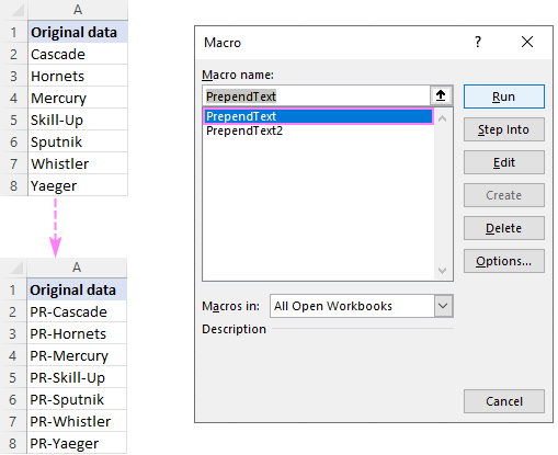
Prepend text to beginning
The below macros add text or a specific character to the beginning of all selected cells. Both codes rely on the same logic: check each cell in the selected range and if the cell is not empty, prepend the specified text. The difference is where the result is placed: the first code makes changes to the original data while the second one places the results in a column to the right of the selected range.
If you have little experience with VBA, this step-by-step guide will walk you through the process: How to insert and run VBA code in Excel.
Macro 1: adds text to the original cells
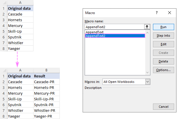
This code inserts the substring «PR-» to the left of an existing text. Before using the code in your worksheet, be sure to replace our sample text with the one you really need.
Macro 2: places the results in the adjacent column
Before running this macro, make sure there is an empty column to the right of the selected range, otherwise the existing data will be overwritten.

Append text to end
If you are looking to add a specific string/character to the end of all selected cells, these codes will help you get the work done quickly.
Macro 1: appends text to the original cells
Our sample code inserts the substring «-PR» to the right of an existing text. Naturally, you can change it to whatever text/character you need.

Macro 2: places the results in another column
This code places the results in a neighboring column. So, before you run it, make certain you have at least one empty column to the right of the selected range, otherwise your existing data will be overwritten.
Add text or character to multiple cells with Ultimate Suite
In the first part of this tutorial, you’ve learned a handful of different formulas to add text to Excel cells. Now, let’s me show you how to accomplish the task with a few clicks 🙂
With Ultimate Suite installed in your Excel, here are the steps to follow:
- Select your source data.
- On the Ablebits tab, in the Text group, click Add.
- On the Add Text pane, type the character/text you wish to add to the selected cells, and specify where it should be inserted:
- At the beginning
- At the end
- Before specific text/character
- After specific text/character
- After Nth character from the beginning or end
- Click the Add Text button. Done!
As an example, let’s insert the string «PR-» after the «-» character in cells A2:A7. For this, we configure the following settings:
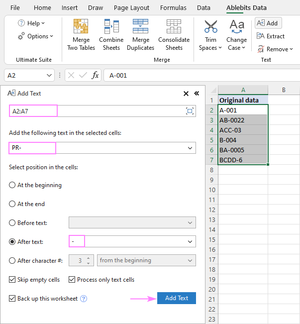
A moment later, we get the desired result:

These are the best ways to add characters and text strings in Excel. I thank you for reading and hope to see you on our blog next week!
Источник
This post explains that how to add the specified text or characters to the beginning of all cells in excel. How to create an excel formula to add same text string or characters to the beginning of text string in one Cell. How to create an excel macro to add specific text to the beginning of the text in all of cells.
Table of Contents
- Add text to the beginning of all cells with Formula
- Add text to the beginning of all cells with Excel VBA
- Related Formulas
- Related Functions
If you want to add the specific text or characters into the beginning of the text in one cell or all cells, you can create an excel formula based on the concatenate operator or CONCATENATE function.
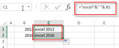
Assuming that you want to add text “excel” into the beginning of the text in Cell B1, you can write down the following formula:
="excel"&" "& B2
OR
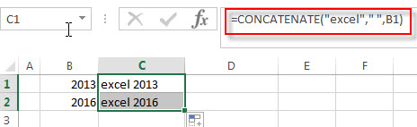
=CONCATENATE(“excel”,””,B1)
You can enter the above formulas in Cell C1, and then drag the fill handle down to other cells in column C and you will see that the specific text will add the beginning of the text in Cell B1.
Add text to the beginning of all cells with Excel VBA
You can create a new excel macro to add text string “excel” to the beginning of text in Cell B1 in Excel VBA, just refer to the below steps:
1# click on “Visual Basic” command under DEVELOPER Tab.

2# then the “Visual Basic Editor” window will appear.
3# click “Insert” ->”Module” to create a new module

4# paste the below VBA code into the code window. Then clicking “Save” button.
Sub addTextAtBeginningCell()
    Dim r As Range
    For Each r In Selection
        If r.Value <> "" Then r.Value = "excel " & r.Value
    Next
End Sub
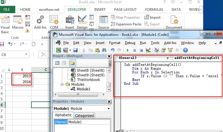
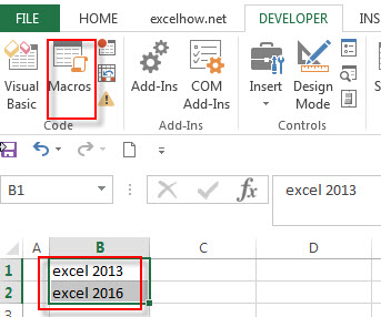
5# back to the current worksheet, then run the above excel macro, you will see that the specific text “excel” has been added into the beginning of the text in all selected Cells.
- How to add text to the end all cells
To add the specified text string or characters to the end of all selected cells in excel, you can use the concatenate operator or the CONCATENATE function to create an excel formula..… - How to join text from two or more cells into one cell separated by commas, space
You can merge text from two or more cells into one cell using a combination of the SUBSTITUTE function, the TRIM function and concatenation operator to create an excel formula..… - Combine columns without losing data
How to keep all data after merging columns. You can use the concatenate operator or CONCATENATE function to create an excel formula. Assuming that you want to merge column B and C into column D, you can use the following formulas:=B2&C2 OR =CONCATENATE(B2, “ “ ,C2).… - How to Extract Text between Commas
To extract text between commas in Cell B1, you can use the following formula based on the SUBSTITUTE function, the MID function and the REPT function.… - How to Combine Text from Two or More Cells into One Cell
If you want to join the text from multiple cells into one cell, you also can use the CONCATENATE function instead of Ampersand operator..…
- Excel Concat function
The excel CONCAT function combines 2 or more strings or ranges together.This is a new function in Excel 2016 and it replaces the CONCATENATE function.The syntax of the CONCAT function is as below:=CONCAT (text1,[text2],…)…
In order to make sure that the data in your Excel file is organized in a way that makes sense, you will want to add some text to the beginning or end of all cells. This is not just for aesthetic purposes—it’s also important because it will help you keep track of what the data means.
In some cases, you may need to add text to the beginning of all cells in Excel. For example, if you have a list of addresses and you want to include each address with its corresponding city name, then adding Address or City to the beginning of all cells will be useful.
Information provided in this article are compatible with versions 2010/2016/MAC/online.
The CONCAT and CONCATENATE Function
CONCAT AND CONCATENATE function are very helpful if you wish to add a certain title in the beginning or end of a list. Here, I will show you an example of adding “Dr.” to the beginning of a list of names.
1. Type “=con” in the target cell and choose if you want to use the CONCAT or the CONCATENATE function. Double-click on the chosen function.
2. Type the argument as the text you want to add in inverted commas (“”) and choose the cell you wish to add after it.
3. Press enter.
4. It’s time to duplicate this formula in the remaining column’s cells. Just click twice on the fill handle or hold and drag it down (located at the bottom right of cell the here B2).
5. You can see that it adds the prefix you want to add to all the cells, as far as you drag down.
6. Alternatively, Ctrl+C (copy) and Ctrl+V (paste) on keyboard can be used for shorter lists, that is copying and pasting the formula onto other cells.
Adding Text Using Ampersand Operator (&)
1.The & operator can also be used to add text in the beginning or end of many cells. Let’s discuss an example where you need to add the percentage sybol (%) after a lot of numbers.
2. Just type in “=” and the formula as shown.
3. The result would look like this when you press enter.
4. If you want a space between the number and the symbol, you can go about two following ways:
5. Note that the space is added before the symbol.
6. To duplicate this formula in the remaining column’s cells, just click twice on the fill handle at the bottom-right corner of each cell or hold and drag it down. Or use Ctrl+C (copy) and Ctrl+V (paste) on keyboard for shorter lists.
The Flash Fill Option
1.If you wish to fill many cells with the same prefix, the Flash fill option can be very useful.
2. Under the ‘Data’ option in the main menu, a ‘Fill’ drop-down menu is availabele that has the ‘Flash Fill’ option.
3. Click on the text you want to fill onto the other cells and click on the Flash Fill option. The data will be copied onto the other cells related to the data. A shortcut of Flash Fill is Ctrl+E on keyboard.
Did you learn about How To Add Text To Beginning Or End Of All Cells In Excel? You can follow WPS Academy to learn more features of Word Document, Excel Spreadsheets and PowerPoint Slides.
You can also download WPS Office to edit the word documents, excel, PowerPoint for free of cost. Download now! And get an easy and enjoyable working experience.