
Excel for Microsoft 365 Excel 2021 Excel 2019 Excel 2016 Excel 2013 Excel 2010 Excel 2007 More…Less
Let’s say you need to create a grammatically correct sentence from several columns of data to prepare a mass mailing. Or, maybe you need to format numbers with text without affecting formulas that use those numbers. In Excel, there are several ways to combine text and numbers.
Use a number format to display text before or after a number in a cell
If a column that you want to sort contains both numbers and text—such as Product #15, Product #100, Product #200—it may not sort as you expect. You can format cells that contain 15, 100, and 200 so that they appear in the worksheet as Product #15, Product #100, and Product #200.
Use a custom number format to display the number with text—without changing the sorting behavior of the number. In this way, you change how the number appears without changing the value.
Follow these steps:
-
Select the cells that you want to format.
-
On the Home tab, in the Number group, click the arrow .

-
In the Category list, click a category such as Custom, and then click a built-in format that resembles the one that you want.
-
In the Type field, edit the number format codes to create the format that you want.
To display both text and numbers in a cell, enclose the text characters in double quotation marks (» «), or precede the numbers with a backslash ().
NOTE: Editing a built-in format does not remove the format.

|
To display |
Use this code |
How it works |
|---|---|---|
|
12 as Product #12 |
«Product # » 0 |
The text enclosed in the quotation marks (including a space) is displayed before the number in the cell. In the code, «0» represents the number contained in the cell (such as 12). |
|
12:00 as 12:00 AM EST |
h:mm AM/PM «EST» |
The current time is shown using the date/time format h:mm AM/PM, and the text «EST» is displayed after the time. |
|
-12 as $-12.00 Shortage and 12 as $12.00 Surplus |
$0.00 «Surplus»;$-0.00 «Shortage» |
The value is shown using a currency format. In addition, if the cell contains a positive value (or 0), «Surplus» is displayed after the value. If the cell contains a negative value, «Shortage» is displayed instead. |
Combine text and numbers from different cells into the same cell by using a formula
When you do combine numbers and text in a cell, the numbers become text and no longer function as numeric values. This means that you can no longer perform any math operations on them.
To combine numbers, use the CONCATENATE or CONCAT, TEXT or TEXTJOIN functions, and the ampersand (&) operator.
Notes:
-
In Excel 2016, Excel Mobile, and Excel for the web, CONCATENATE has been replaced with the CONCAT function. Although the CONCATENATE function is still available for backward compatibility, you should consider using CONCAT, because CONCATENATE may not be available in future versions of Excel.
-
TEXTJOIN combines the text from multiple ranges and/or strings, and includes a delimiter you specify between each text value that will be combined. If the delimiter is an empty text string, this function will effectively concatenate the ranges. TEXTJOIN is not available in Excel 2013 and previous versions.
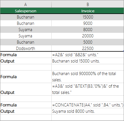
Examples
See various examples in the figure below.
Look closely at the use of the TEXT function in the second example in the figure. When you join a number to a string of text by using the concatenation operator, use the TEXT function to control the way the number is shown. The formula uses the underlying value from the referenced cell (.4 in this example) — not the formatted value you see in the cell (40%). You use the TEXT function to restore the number formatting.
Need more help?
You can always ask an expert in the Excel Tech Community or get support in the Answers community.
See Also
-
CONCATENATE function
-
CONCAT function
-
TEXT function
-
TEXTJOIN function
Need more help?
There may be times when you need to insert the identical text into all of the cells that are contained inside a column. It’s possible that a specific title needs to go before the names in a list, or that a specific symbol needs to go at the end of the text in each cell. Both of these things need to be done. The task of adding text or numbers to cells in Excel is one of the most often performed tasks. Including things like inserting spaces between names, including prefixes and suffixes in cells, and inserting dashes in social security numbers.
Excel provides some extremely simple ways that you can add text to the beginning or end of the text that is present in a range of cells. These can be done independently of one another.
In this tutorial, you are going to learn about some methods to add text into specified position of cell.
Using ampersand (&) Operator
A useful feature of the operator represented by the ampersand (&) is to combine many text strings into a single one.
Let’s see one example and understand step by step how we can add text in a specific position in a cell.
Step 1
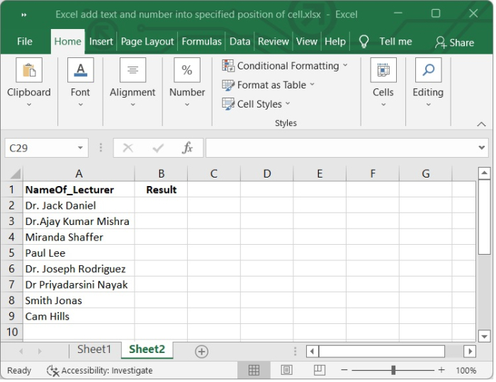
In our example, we have name of some lecturer who are promoted to get a position of professor. We have to add Professor before their name.
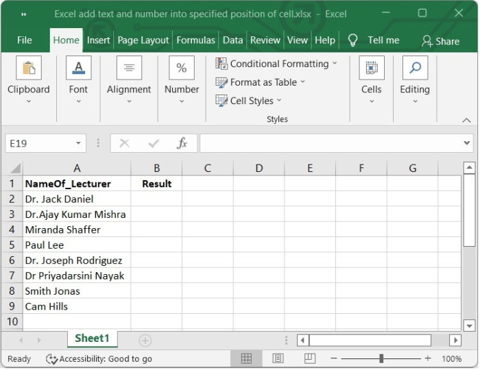
Step 2
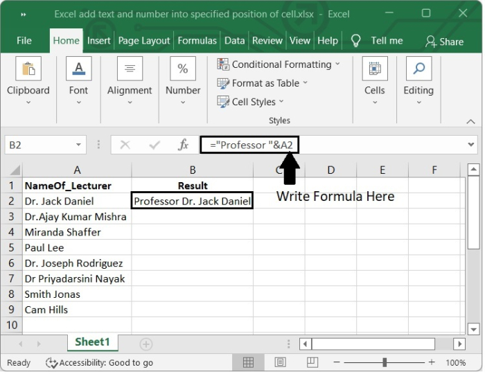
Select one blank cell and write the following formula to add text before the name. In our example we have selected the cell B2 and written the formula to add Professor before the name of the lecturers there.
="text "&cell
In our example, we have written the following formula
="Professor "&A2
After pressing Enter, we will see the text Professor has been added before
the names.
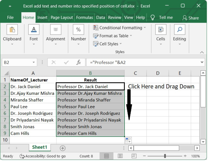
Step 3
To get the result in all the remaining cells, click on the ‘+’ sign appears on the lower right corner of the cell B2, which activates the autofill function and then drag down.
Using CONCATENATE Function
Excel’s CONCATENATE function is a very useful one since it enables users to insert text both at the beginning and the end of a string of text. In terms of the functionality that it provides, the CONCATENATE() function is
comparable to the ampersand (&) operator. The only distinction between the two is in the manner in which they are utilized. This function is applicable to us at the beginning to the end of the text.
Add text at the beginning of cell
Step 1
In our example, we have the names of some professors who used to be lecturers. We need to put «Professor» in front of their name. See the following image.
Step 2
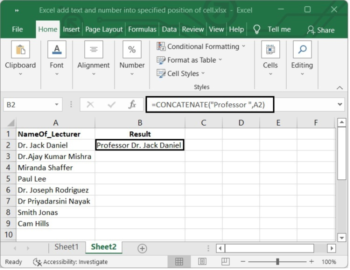
We want to add text at the beginning of the names. To add at the beginning of the names, write the following formula at the formula bar.
=CONCATENATE("TEXT",cell)
In our example, we want to add the text “Professor” at the beginning
=CONCATENATE("Professor ",A2)
After pressing enter, we will see the text Professor has been added before the names. See the following image.
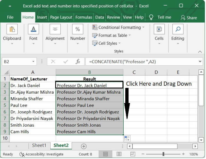
Step 3
To get the result in all the other cells, click the «+» sign in the lower right corner of cell B2. This turns on the autofill feature, and you can then drag down. See the following image.
Add text at the end of cell
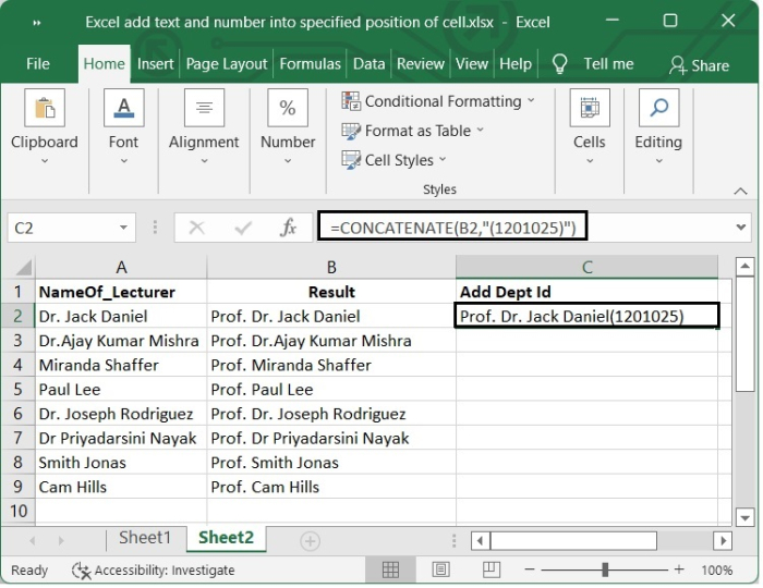
Let’s suppose we want to add the department id at the end of the names of the professors given in above example.
Step 1
Write the following formula to add the text at the end of the cell.
= CONCATENATE(Cell,"Text")
In our example we are writing the following formula and press enter.
=CONCATENATE(B2,"(1201025)")
See the following image.
Step 2
Choose cell C2, drag the Fill Handle down to the cell you want to fill with this formula. See the below picture.

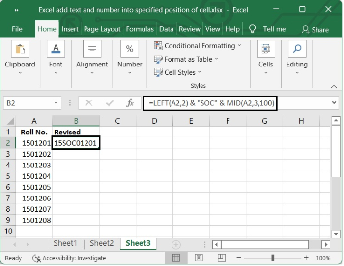
Add Text in Middle of Cell
Step 1
In our example, we have some Roll Numbers in our Excel sheet and we want to add SOC in the middle of the roll no. See the following image.
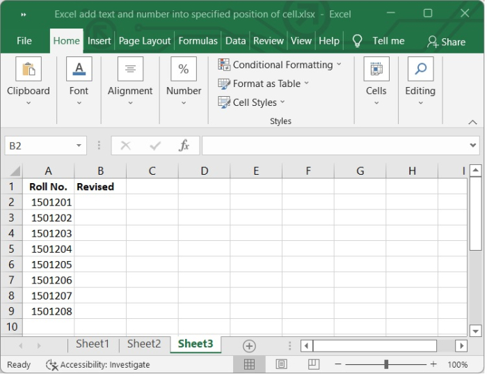
Step 2
To add SOC in the middle of the Roll No., write the following formula and press enter.
=LEFT(A2,2) & "SOC" & MID(A2,3,100)
See the following image.
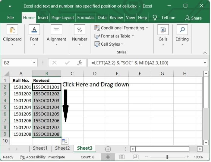
Step 3
Choose cell B2, drag the Fill Handle down to the cell you want to fill with this formula.
Conclusion
In this tutorial, you learnt how to add text and number into a specified position of cell in Excel.
Combining Text and Numbers from Separate Cells
We begin with a small table that contains names (text) in column A and amounts (numbers) in column B.

Our goal is to have the name and amount for each row of the table displayed in a single cell (column C).
This needs to be done dynamically so that a change in either the name or amount will trigger an update in the combined version in column C.
This can be accomplished with a CONCATENATE function.
CONCATENATE is a big, fancy word for “join things together”.
Excel has a dedicated CONCATENATE function, but most users will opt to use the simplified version of CONCATENATE… the ampersand (&) symbol.
For example, we begin in cell C2 and write the following formula:
=A2 & B2
Pressing ENTER to commit the formula results in the following:

This is the purest form of concatenation; everything is just smashed together. It works, but it’s not visually appealing.
Concatenation is not limited to existing content. We can inject new content into the formula to enhance the results. In our case, we’ll inject a ‘space’ to provide visual padding between the name and the amount.
The ‘space’ needs to be surrounded by double-quotes. Any injected text needs to be surrounded by double-quotes.
=A2 & " " & B2
The updated formula’s result is a bit easier to read.

Think of the ampersand character as the word “and”. “Display the name in cell A2 and a space and the number in cell B2.”
You can place anything you wish between the two double-quotes, like a dash, slash, or any other character.


Returning to using a ‘space’, we fill the formula down to the remaining rows to reveal the following:

Formatting the Numbers in the Result
If we need to represent the numbers in the result as money (we’ll use U.S. Dollars in our example) we can’t just click the dollar sign button on the ribbon. The formatting codes for Currency Style are rendered inert with the presence of the concatenated text.
But not to worry; we have a solution.
We can apply number formatting to the result via the TEXT function.
The Excel TEXT function has the following syntax:
=TEXT(value, format_text)- value – This can be a static value, a reference to a cell that contains a value, or a formula that returns a value.
- format_text – This is the formatting code(s) that determine the way numbers are presented.
For our numbers, we want to display a dollar sign and a comma for every three place values. We also want to show zero if the number is zero.
Our codes for this are:
“$#,##0”
The formatting codes are always placed within a set of double-quotes.
Our formula would be updated as follows:
=A2 & " " & TEXT(B2, "$#,##0")
Committing our new formula to all rows of the tale gives us a much more appealing result.

As the values in column B change, the TEXT functions in column C will apply the appropriate number formatting.
For more information on the formatting codes and uses in the TEXT function, visit the following link.
Microsoft Excel’s TEXT Function
PRO TIP:
If you are unsure what formatting codes to use, an easy way to figure it out is to do the following:
- Select a cell with the number you want to format (ex: cell B2) and press F1 to open the number formatting dialog box.
- Select the category (on the left) then the desired formatting (on the right).

- Select the “Custom” category (on the left) to reveal the underlying codes needed to support the selection from Step 2.

By applying different formatting options and examining the underlying codes, you will likely figure out many of the symbol’s purposes.
Using Aggregation Functions Inside a Formatting Function

Because the first argument in the TEXT function can be a formula, we can embed an aggregation function, like SUM, into the formula to produce a formatted aggregation.
="Base: " & TEXT(SUM(B2:B5), "$#,##0")
The SUM function provides the aggregation which is then passed off to the TEXT function that applies the formatting codes.
The final touch is to concatenate the text string “Base: ” to the front of the formatted number.
We can write a similar formula for the bonus column.
="Bonus: " & TEXT(SUM(B2:B5), "$#,##0")“What if we want to add the ‘Base” and ‘Bonus’ results?”
If we write a SUM function that attempts to aggregate the results of the previous two formulas, we end up with a less than desirable result.


This occurs because we have embedded text in the same cell as the result of the SUM function.
Separating the Formatting from the Aggregation
We can overcome the previous issue by concatenating the desired text in a Custom Number Format to produce the same result.
This allows you to place a simple aggregation function, like SUM, in a cell without any other modifiers.

We can then select the cell containing the above formula, press F1 to open the Format Cells dialog box and apply the following custom number format.
"Base: "$#,##0
We can apply a similar formatting code sequence to the bonus columns total in cell C6.

"Bonus: "$#,##0Adding the two SUM results now works perfectly.

NOTE: I applied the following Custom Number Format to the result to spice it up like the other aggregations.
"Total: "$#,##0Practice Workbook
Feel free to Download the Workbook HERE.
![]()
Published on: January 14, 2022
Last modified: March 17, 2023


Leila Gharani
I’m a 5x Microsoft MVP with over 15 years of experience implementing and professionals on Management Information Systems of different sizes and nature.
My background is Masters in Economics, Economist, Consultant, Oracle HFM Accounting Systems Expert, SAP BW Project Manager. My passion is teaching, experimenting and sharing. I am also addicted to learning and enjoy taking online courses on a variety of topics.
In all versions of Excel, you can use a simple formula, with the & operator, to combine values from different cells. If you want the numbers formatted a certain way, use the TEXT function to set that up.
Video: Combine Text and Numbers
First, this video shows a simple formula to combine text and numbers in Excel. Then, see how to use the Excel TEXT function, to format the numbers in the formula.
You can type the formatting information inside the TEXT function. Or, put the formatting string in a different cell, and refer to that cell in the TEXT function.
To follow along, get the sample file on my Contextures site – How to Combine Cells
TEXTJOIN – Excel 365
If you’re using Excel 365, there’s a new TEXTJOIN function. It makes it easy to combine values from multiple cells.
This short video shows a couple of TEXTJOIN examples. First, see a simple formula to combine weekday names. Next, use the TEXT function inside TEXTJOIN, create formatted dates. There are written steps, and more examples, on my Contextures website.
Simple Formula
Even if you don’t have the new TEXTJOIN function, it’s easy combine values from multiple cells, using a simple formula. Just use the & (ampersand) operator, to join values together.
In this example:
- There’s text in cell A2, with a space character at the end.
- There’s an unformatted number in cell B2.
This formula, in cell C2, combines the text and number:
=A2 & B2
Or, if the text does not have a space character at the end, add one in the formula
=A2 & " " & B2

Format Numbers with TEXT Function
To join text with formatted numbers, use the TEXT function in the formula.
In this example:
- There’s text in cell A2, with a space character at the end.
- There’s a formatted date in cell B2.
This formula, in cell C2, combines the text and date, with formatting:
=A2 & TEXT(B2,"d-mmm")

Number Format Information
Instead of typing the number format inside the TEXT function, you could type those formats in another column, or on a different worksheet.
Then, in the TEXT function, refer to the cell with the required format.
For example, I’ve made a formatting list with named cells. Now, I can use those names in the TEXT function.
- FmtDMY d-mmm-yyyy
- FmtCurr $#,##0
- FmtFrac # ?/?

In this example, the formula in C2 uses the d-mmm-yyyy format, from the cell named FmtDMY:
=A2 & TEXT(B2,FmtDMY)
The other named formats are used in cells C5 and C8.
Currency – cell C5
=A5 & TEXT(B5,FmtCurr)
Fraction – cell C8
=A8 & TEXT(B8,FmtFrac)

Get the Workbook
To see more examples of combining text and numbers, and to get the sample workbook, go to the Combine Cells page on my Contextures site.
The zipped file is in xlsx format, and does not contain any macros.
________________________________
Combine Text and Formatted Numbers in Excel


________________________________
In this article, we will learn How to Combine Text and Formatted Numbers into a Single Entity in Excel in Excel.
Scenario:
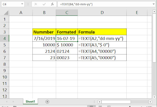
Excel considers number values in many formats like number, date, time, text, percentage or currency. These can be changed into each other. Excel converts numbers to text to use numbers as text in formulas like vlookup with numbers and text. The Excel TEXT function lets you convert the number to text. The TEXT function in Excel is used to convert numbers into text. The fun part is you can format that number to show it in the desired format. For example format a yy-mm-dd date into dd-mm-yy format. Add currency signs before a number and many more.
TEXT formula in Excel
TEXT function is a string function which converts any value to a given format. The result may seem that it is a number but it’s in text format.
=TEXT(cell_ref, text_format)
cell_ref : value to convert using cell reference
Text_format : Format to convert
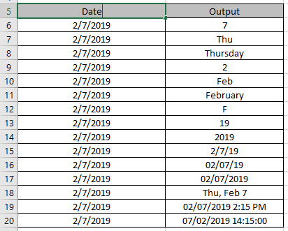
| Format | Output_format |
| d | 7 |
| ddd | Thu |
| dddd | Thursday |
| m | 2 |
| mmm | Feb |
| mmmm | February |
| mmmmm | F |
| yy | 19 |
| yyyy | 2019 |
| m/d/y | 2/7/19 |
| mm/dd/yy | 02/07/19 |
| mm/dd/yyyy | 02/07/2019 |
| ddd, mmm d | Thu, Feb 7 |
| mm/dd/yyyy h:mm AM/PM | 02/07/2019 2:15 PM |
| mm/dd/yyyy hh:mm:ss | 07/02/2019 14:15:00 |
Example :
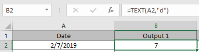
All of these might be confusing to understand. Let’s understand how to use the function using an example. Here we have some examples to convert date values to text format or any other required format.
Convert the value in A2 cell.
Use the formula in C2 cell
“0”: returns the general text format.
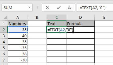
Press Enter and copy the formula in remaining cells using Ctrl + D
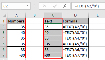
As you can see we got numbers as text output because the significance number always varied.
Here we have some numbers to convert to text format or any other required format.
Use the formula:
As you can see the value in the output cell is in Text format.
You can use any Format_text and do your work in excel without any interruption
Add 0 before a Number
Sometimes you are needed to add 0 before some fixed digit of numbers like phone number or pin number. Use this Text formula to do so…
If you have N digits of number then in text format argument write n+1 0s.
Add Currency Before a Number
Write this text formula to add currency.
As you can see we got numbers as text output because the significance number always varied.
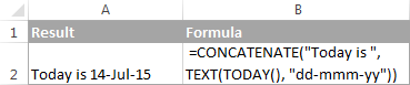
Concatenating a text string and a formula-calculated value. To make the result returned by some formula more understandable for your users, you can concatenate it with a text string that explains what the value actually is.
For example, you can use the following formula to return the current date:
=CONCATENATE(«Today is «,TEXT(TODAY(), «dd-mmm-yy»))
Using CONCATENATE in Excel — things to remember
To ensure that your CONCATENATE formulas always deliver the correct results, remember the following simple rules:
Excel CONCATENATE function requires at least one «text» argument to work.
Here are all the observational notes using the formula in Excel
Notes :
- Use & operator to combine text. & operator does the same work as CONCAT function
- In new versions of Excel, CONCATENATE is replaced with the CONCAT function, which has exactly the same syntax. The CONCATENATE function is kept for backward compatibility, it is common practice to use CONCAT instead because Excel does not give any promises that CONCATENATE will be available in future versions of Excel.
Hope this article about How to Combine Text and Formatted Numbers into a Single Entity in Excel in Excel is explanatory. Find more articles on calculating values and related Excel formulas here. If you liked our blogs, share them with your friends on Facebook. And also you can follow us on Twitter and Facebook. We would love to hear from you, do let us know how we can improve, complement or innovate our work and make it better for you. Write to us at info@exceltip.com.
Related Articles :
Excel REPLACE vs SUBSTITUTE function: The REPLACE and SUBSTITUTE functions are the most misunderstood functions. To find and replace a given text we use the SUBSTITUTE function. Where REPLACE is used to replace a number of characters in a string.
How to use the ISTEXT function in Excel : returns the TRUE logic value if the cell value is text using the ISTEXT function in Excel.
How to Highlight cells that contain specific text in Excel : Highlight cells based on the formula to find the specific text value within the cell in Excel.
Converts decimal Seconds into time format : As we know that time in excel is treated as numbers. Hours, Minutes, and Seconds are treated as decimal numbers. So when we have seconds as numbers, how do we convert into time format? This article got it covered.
Calculate Minutes Between Dates & Time in Excel : calculating the time difference is quite easy. Just need to subtract the start time from the end time. Learn more about this formula clicking the link
Replace text from end of a string starting from variable position : To replace text from the end of the string, we use the REPLACE function. The REPLACE function use the position of text in the string to replace.
Popular Articles :
50 Excel Shortcuts to Increase Your Productivity : Get faster at your tasks in Excel. These shortcuts will help you increase your work efficiency in Excel.
How to use the VLOOKUP Function in Excel : This is one of the most used and popular functions of excel that is used to lookup value from different ranges and sheets.
How to use the IF Function in Excel : The IF statement in Excel checks the condition and returns a specific value if the condition is TRUE or returns another specific value if FALSE.
How to use the SUMIF Function in Excel : This is another dashboard essential function. This helps you sum up values on specific conditions.
How to use the COUNTIF Function in Excel : Count values with conditions using this amazing function. You don’t need to filter your data to count specific values. Countif function is essential to prepare your dashboard.
If you want to combine text with the results of a formula in a cell, you can use concatenation. Suppose you have calculated the total of a range of cells using a formula in cell D2. Now, you want to have cell A2 display the text «Today’s sales are $12,000», where $12,000 is the value calculated in D2. As the value in D2 changes, you want the value in A2 to update automatically.
For example, suppose you have calculated the total of a range of cells using a formula in cell D2. Now, you want to have cell A2 display the text «Today’s sales are $12,000», where $12,000 is the value calculated in D2. As the value in D2 changes, you want the value in A2 to update automatically.
To do this, type the following formula into A2:
=»Today’s sales are $»&D2
The secret here is to use the ampersand, &, to concatenate (or join) text and numbers together. The & symbol acts like a +, or plus sign, to join text strings together into one. A slightly more advanced version of the formula above might look like the following:
=»You owe $»&D2&», which is due in 7 days»
You can also use the CONCATENATE() function to join multiple text strings together. The syntax of this function is as follows:
=CONCATENATE(text1,text2,…)
In this function, you can join up to 30 text strings together. To achieve the same result as the first example above, you could enter the following formula:
=CONCATENATE(«Today’s sales are $»,d2)
.
Excel is a great tool for doing all the analysis and finalizing the report. But sometimes, calculation alone cannot convey the message to the reader because every reader has their way of looking at the report. Some people can understand the numbers just by looking at them, some need some time to get the real story, and some cannot understand. So, they need a full and clear-cut explanation of everything.
You can download this Text in Excel Formula Template here – Text in Excel Formula Template
To bring all the users to the same page while reading the report, we can add text comments to the formula to make the report easily readable.
Let us look at how we can add text in Excel formulas.
Table of contents
- Formula with Text in Excel
- #1 – Add Meaningful Words Using with Text in Excel Formula
- #2 – Add Meaningful Words to Formula Calculations with TIME Format
- #3 – Add Meaningful Words to Formula Calculations with Date Format
- Things to Remember Formula with Text in Excel
- Recommended Articles
#1 – Add Meaningful Words Using Text in Excel Formula
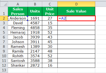
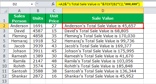
Often in Excel, we only perform calculations. Therefore, we are not worried about how well they convey the message to the reader. For example, take a look at the below data.
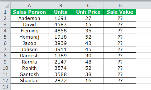
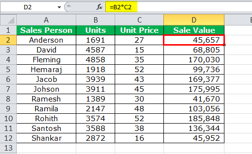
By looking at the above image, it is very clear that we need to find the sale value by multiplying Units to Unit PriceUnit Price is a measurement used for indicating the price of particular goods or services to be exchanged with customers or consumers for money. It includes fixed costs, variable costs, overheads, direct labour, and a profit margin for the organization.read more.
Apply simple text in the Excel formula to get the total sales value for each salesperson.
Usually, we stop the process here itself.
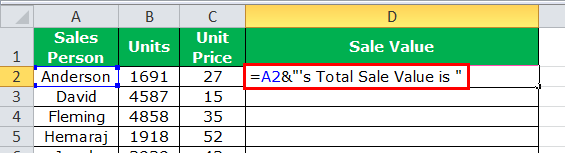
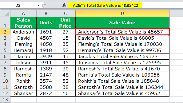
How about showing the calculation as Anderson’s total “Sale Value” is 45,657?
It looks like a complete sentence to convey a clear message to the user. So, let us go ahead and frame a sentence along with the formula.
So, let us go ahead and frame a sentence along with the formula.
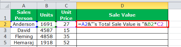
- We know the format of the sentence to be framed. Firstly, we need a “Sales Person” name to appear. So, we must select the cell A2 cell.

- Now, we need “Total Sale Value” after the salesperson’s name. We need to put the ampersand operator sign after selecting the first cell to comb this text value.

- Now, we need to do the calculation to get the sale value. Put on more (ampersand) sign and apply the formula as B*C2.

- Now, we must press the “Enter” key to complete the formula and our text values.

One problem with this formula is that sales numbers are not formatted properly. Because they do not have a thousand separators, that would have made the numbers look properly.
There is nothing to worry about; we can format the numbers with the TEXT function in the Excel formula.
Edit the formula. As shown below, the calculation part applies the Excel TEXT function to format the numbers.

Now, we have the proper format of numbers along with the sales values. The TEXT function in Excel formula format the calculation (B2*C2) to the format of ###, ###.
#2 – Add Meaningful Words to Formula Calculations with TIME Format
We have seen how to add text values to our formulas to convey a clear-cut message to the readers or users. Now, we will be adding text values to another calculation, which includes time calculations.
We have data on flight departure and arrival timings. We need to calculate the total duration of each flight.
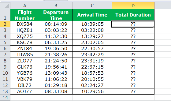
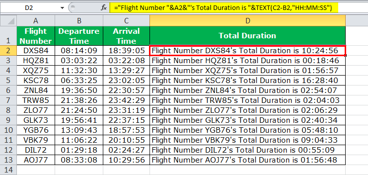
Not only the total duration, but we want to show the message like this “Flight Number DXS84’s total duration is 10:24:56.”
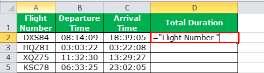
In cell D2, we must start the formula. Our first value is “Flight Number.” We must enter this in double-quotes.
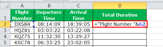
The next value we need to add is the flight number already in cell A2. Enter the “&” symbol and select cell A2.
The next thing we need to add to the text‘s “Total Duration.”We must insert one more “&”symbol and enter this text in double-quotes.
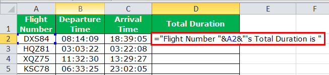
Now comes the most important part of the formula. We need to calculate the total duration after “&” the symbol enters the formula as C2 – B2.
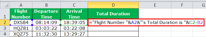
Our full calculation is complete. Press the “Enter” key to get the result.
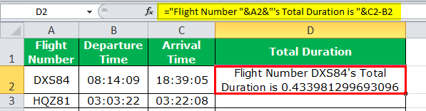
We got the total duration as 0.433398, which is not in the right format. So, we must apply the TEXT function to perform the calculation and format that to TIME.
#3 – Add Meaningful Words to Formula Calculations with Date Format
The TEXT function can perform the formatting task when adding text values to get the correct number format. Now, we will see it in the date format.
Below is the daily sales table that we update the values regularly.
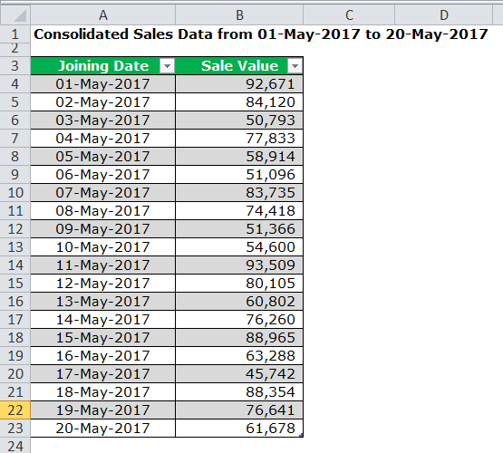
We need to automate the heading as the data keeps adding, i.e., we should change the last date as per the last day of the table.
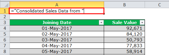
Step 1: We must first open the formula in the A1 cell as “Consolidated Sales Data from.”
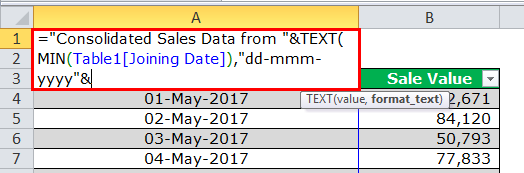
Step 2: Put the “&” symbol and apply the TEXT function in the Excel formula. Apply the MIN function to get the least date from this list inside the TEXT function. And format it as “dd-mmm-yyyy.”
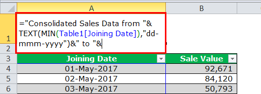
Step 3: Now, enter the word to.
Step 4: To get the latest date from the table, we must apply the MAX formulaThe MAX Formula in Excel is used to calculate the maximum value from a set of data/array. It counts numbers but ignores empty cells, text, the logical values TRUE and FALSE, and text values.read more, and format it as the date by using TEXT in the Excel formula.
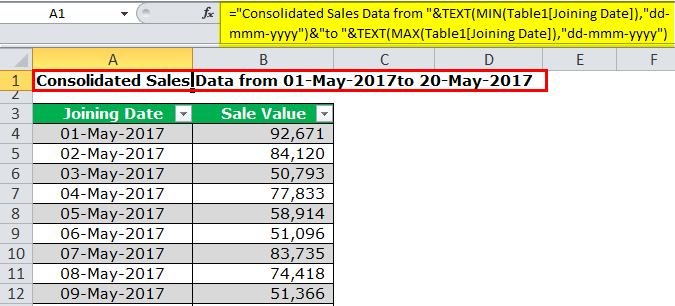
As we update the table, it will automatically update the heading.
Things to Remember Formula with Text in Excel
- We can add the text values according to our preferences by using the CONCATENATE function in excelThe CONCATENATE function in Excel helps the user concatenate or join two or more cell values which may be in the form of characters, strings or numbers.read more or the ampersand (&) symbol.
- To get the correct number format, we must use the TEXT function and specify the number format we want to display.
Recommended Articles
This article has been a guide on Text in Excel Formula. Here, we discuss how to add text in the Excel formula cell along with practical examples and downloadable Excel templates. You may also look at these useful functions in Excel: –
- Separate Text in Excel
- How to Wrap Text in Excel?
- How to Convert Text to Numbers in Excel?
- Convert Date to Text in Excel