
Many users find that using an external keyboard with keyboard shortcuts for Excel helps them work more efficiently. For users with mobility or vision disabilities, keyboard shortcuts can be easier than using the touchscreen and are an essential alternative to using a mouse.
Notes:
-
The shortcuts in this topic refer to the US keyboard layout. Keys for other layouts might not correspond exactly to the keys on a US keyboard.
-
A plus sign (+) in a shortcut means that you need to press multiple keys at the same time.
-
A comma sign (,) in a shortcut means that you need to press multiple keys in order.
This article describes the keyboard shortcuts, function keys, and some other common shortcut keys in Excel for Windows.
Notes:
-
To quickly find a shortcut in this article, you can use the Search. Press Ctrl+F, and then type your search words.
-
If an action that you use often does not have a shortcut key, you can record a macro to create one. For instructions, go to Automate tasks with the Macro Recorder.
-
Download our 50 time-saving Excel shortcuts quick tips guide.
-
Get the Excel 2016 keyboard shortcuts in a Word document: Excel keyboard shortcuts and function keys.
In this topic
-
Frequently used shortcuts
-
Ribbon keyboard shortcuts
-
Use the Access keys for ribbon tabs
-
Work in the ribbon with the keyboard
-
-
Keyboard shortcuts for navigating in cells
-
Keyboard shortcuts for formatting cells
-
Keyboard shortcuts in the Paste Special dialog box in Excel 2013
-
-
Keyboard shortcuts for making selections and performing actions
-
Keyboard shortcuts for working with data, functions, and the formula bar
-
Keyboard shortcuts for refreshing external data
-
Power Pivot keyboard shortcuts
-
Function keys
-
Other useful shortcut keys
Frequently used shortcuts
This table lists the most frequently used shortcuts in Excel.
|
To do this |
Press |
|---|---|
|
Close a workbook. |
Ctrl+W |
|
Open a workbook. |
Ctrl+O |
|
Go to the Home tab. |
Alt+H |
|
Save a workbook. |
Ctrl+S |
|
Copy selection. |
Ctrl+C |
|
Paste selection. |
Ctrl+V |
|
Undo recent action. |
Ctrl+Z |
|
Remove cell contents. |
Delete |
|
Choose a fill color. |
Alt+H, H |
|
Cut selection. |
Ctrl+X |
|
Go to the Insert tab. |
Alt+N |
|
Apply bold formatting. |
Ctrl+B |
|
Center align cell contents. |
Alt+H, A, C |
|
Go to the Page Layout tab. |
Alt+P |
|
Go to the Data tab. |
Alt+A |
|
Go to the View tab. |
Alt+W |
|
Open the context menu. |
Shift+F10 or Windows Menu key |
|
Add borders. |
Alt+H, B |
|
Delete column. |
Alt+H, D, C |
|
Go to the Formula tab. |
Alt+M |
|
Hide the selected rows. |
Ctrl+9 |
|
Hide the selected columns. |
Ctrl+0 |
Top of Page
Ribbon keyboard shortcuts
The ribbon groups related options on tabs. For example, on the Home tab, the Number group includes the Number Format option. Press the Alt key to display the ribbon shortcuts, called Key Tips, as letters in small images next to the tabs and options as shown in the image below.
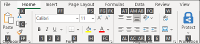
You can combine the Key Tips letters with the Alt key to make shortcuts called Access Keys for the ribbon options. For example, press Alt+H to open the Home tab, and Alt+Q to move to the Tell me or Search field. Press Alt again to see KeyTips for the options for the selected tab.
Depending on the version of Microsoft 365 you are using, the Search text field at the top of the app window might be called Tell Me instead. Both offer a largely similar experience, but some options and search results can vary.
In Office 2013 and Office 2010, most of the old Alt key menu shortcuts still work, too. However, you need to know the full shortcut. For example, press Alt, and then press one of the old menu keys, for example, E (Edit), V (View), I (Insert), and so on. A notification pops up saying you’re using an access key from an earlier version of Microsoft 365. If you know the entire key sequence, go ahead, and use it. If you don’t know the sequence, press Esc and use Key Tips instead.
Use the Access keys for ribbon tabs
To go directly to a tab on the ribbon, press one of the following access keys. Additional tabs might appear depending on your selection in the worksheet.
|
To do this |
Press |
|---|---|
|
Move to the Tell me or Search field on the ribbon and type a search term for assistance or Help content. |
Alt+Q, then enter the search term. |
|
Open the File menu. |
Alt+F |
|
Open the Home tab and format text and numbers and use the Find tool. |
Alt+H |
|
Open the Insert tab and insert PivotTables, charts, add-ins, Sparklines, pictures, shapes, headers, or text boxes. |
Alt+N |
|
Open the Page Layout tab and work with themes, page setup, scale, and alignment. |
Alt+P |
|
Open the Formulas tab and insert, trace, and customize functions and calculations. |
Alt+M |
|
Open the Data tab and connect to, sort, filter, analyze, and work with data. |
Alt+A |
|
Open the Review tab and check spelling, add notes and threaded comments, and protect sheets and workbooks. |
Alt+R |
|
Open the View tab and preview page breaks and layouts, show and hide gridlines and headings, set zoom magnification, manage windows and panes, and view macros. |
Alt+W |
Top of Page
Work in the ribbon with the keyboard
|
To do this |
Press |
|---|---|
|
Select the active tab on the ribbon and activate the access keys. |
Alt or F10. To move to a different tab, use access keys or the arrow keys. |
|
Move the focus to commands on the ribbon. |
Tab key or Shift+Tab |
|
Move down, up, left, or right, respectively, among the items on the ribbon. |
Arrow keys |
|
Show the tooltip for the ribbon element currently in focus. |
Ctrl+Shift+F10 |
|
Activate a selected button. |
Spacebar or Enter |
|
Open the list for a selected command. |
Down arrow key |
|
Open the menu for a selected button. |
Alt+Down arrow key |
|
When a menu or submenu is open, move to the next command. |
Down arrow key |
|
Expand or collapse the ribbon. |
Ctrl+F1 |
|
Open a context menu. |
Shift+F10 Or, on a Windows keyboard, the Windows Menu key (usually between the Alt Gr and right Ctrl keys) |
|
Move to the submenu when a main menu is open or selected. |
Left arrow key |
|
Move from one group of controls to another. |
Ctrl+Left or Right arrow key |
Top of Page
Keyboard shortcuts for navigating in cells
|
To do this |
Press |
|---|---|
|
Move to the previous cell in a worksheet or the previous option in a dialog box. |
Shift+Tab |
|
Move one cell up in a worksheet. |
Up arrow key |
|
Move one cell down in a worksheet. |
Down arrow key |
|
Move one cell left in a worksheet. |
Left arrow key |
|
Move one cell right in a worksheet. |
Right arrow key |
|
Move to the edge of the current data region in a worksheet. |
Ctrl+Arrow key |
|
Enter the End mode, move to the next nonblank cell in the same column or row as the active cell, and turn off End mode. If the cells are blank, move to the last cell in the row or column. |
End, Arrow key |
|
Move to the last cell on a worksheet, to the lowest used row of the rightmost used column. |
Ctrl+End |
|
Extend the selection of cells to the last used cell on the worksheet (lower-right corner). |
Ctrl+Shift+End |
|
Move to the cell in the upper-left corner of the window when Scroll lock is turned on. |
Home+Scroll lock |
|
Move to the beginning of a worksheet. |
Ctrl+Home |
|
Move one screen down in a worksheet. |
Page down |
|
Move to the next sheet in a workbook. |
Ctrl+Page down |
|
Move one screen to the right in a worksheet. |
Alt+Page down |
|
Move one screen up in a worksheet. |
Page up |
|
Move one screen to the left in a worksheet. |
Alt+Page up |
|
Move to the previous sheet in a workbook. |
Ctrl+Page up |
|
Move one cell to the right in a worksheet. Or, in a protected worksheet, move between unlocked cells. |
Tab key |
|
Open the list of validation choices on a cell that has data validation option applied to it. |
Alt+Down arrow key |
|
Cycle through floating shapes, such as text boxes or images. |
Ctrl+Alt+5, then the Tab key repeatedly |
|
Exit the floating shape navigation and return to the normal navigation. |
Esc |
|
Scroll horizontally. |
Ctrl+Shift, then scroll your mouse wheel up to go left, down to go right |
|
Zoom in. |
Ctrl+Alt+Equal sign ( = ) |
|
Zoom out. |
Ctrl+Alt+Minus sign (-) |
Top of Page
Keyboard shortcuts for formatting cells
|
To do this |
Press |
|---|---|
|
Open the Format Cells dialog box. |
Ctrl+1 |
|
Format fonts in the Format Cells dialog box. |
Ctrl+Shift+F or Ctrl+Shift+P |
|
Edit the active cell and put the insertion point at the end of its contents. Or, if editing is turned off for the cell, move the insertion point into the formula bar. If editing a formula, toggle Point mode off or on so you can use the arrow keys to create a reference. |
F2 |
|
Insert a note. Open and edit a cell note. |
Shift+F2 Shift+F2 |
|
Insert a threaded comment. Open and reply to a threaded comment. |
Ctrl+Shift+F2 Ctrl+Shift+F2 |
|
Open the Insert dialog box to insert blank cells. |
Ctrl+Shift+Plus sign (+) |
|
Open the Delete dialog box to delete selected cells. |
Ctrl+Minus sign (-) |
|
Enter the current time. |
Ctrl+Shift+Colon (:) |
|
Enter the current date. |
Ctrl+Semicolon (;) |
|
Switch between displaying cell values or formulas in the worksheet. |
Ctrl+Grave accent (`) |
|
Copy a formula from the cell above the active cell into the cell or the formula bar. |
Ctrl+Apostrophe (‘) |
|
Move the selected cells. |
Ctrl+X |
|
Copy the selected cells. |
Ctrl+C |
|
Paste content at the insertion point, replacing any selection. |
Ctrl+V |
|
Open the Paste Special dialog box. |
Ctrl+Alt+V |
|
Italicize text or remove italic formatting. |
Ctrl+I or Ctrl+3 |
|
Bold text or remove bold formatting. |
Ctrl+B or Ctrl+2 |
|
Underline text or remove underline. |
Ctrl+U or Ctrl+4 |
|
Apply or remove strikethrough formatting. |
Ctrl+5 |
|
Switch between hiding objects, displaying objects, and displaying placeholders for objects. |
Ctrl+6 |
|
Apply an outline border to the selected cells. |
Ctrl+Shift+Ampersand sign (&) |
|
Remove the outline border from the selected cells. |
Ctrl+Shift+Underscore (_) |
|
Display or hide the outline symbols. |
Ctrl+8 |
|
Use the Fill Down command to copy the contents and format of the topmost cell of a selected range into the cells below. |
Ctrl+D |
|
Apply the General number format. |
Ctrl+Shift+Tilde sign (~) |
|
Apply the Currency format with two decimal places (negative numbers in parentheses). |
Ctrl+Shift+Dollar sign ($) |
|
Apply the Percentage format with no decimal places. |
Ctrl+Shift+Percent sign (%) |
|
Apply the Scientific number format with two decimal places. |
Ctrl+Shift+Caret sign (^) |
|
Apply the Date format with the day, month, and year. |
Ctrl+Shift+Number sign (#) |
|
Apply the Time format with the hour and minute, and AM or PM. |
Ctrl+Shift+At sign (@) |
|
Apply the Number format with two decimal places, thousands separator, and minus sign (-) for negative values. |
Ctrl+Shift+Exclamation point (!) |
|
Open the Insert hyperlink dialog box. |
Ctrl+K |
|
Check spelling in the active worksheet or selected range. |
F7 |
|
Display the Quick Analysis options for selected cells that contain data. |
Ctrl+Q |
|
Display the Create Table dialog box. |
Ctrl+L or Ctrl+T |
|
Open the Workbook Statistics dialog box. |
Ctrl+Shift+G |
Top of Page
Keyboard shortcuts in the Paste Special dialog box in Excel 2013
In Excel 2013, you can paste a specific aspect of the copied data like its formatting or value using the Paste Special options. After you’ve copied the data, press Ctrl+Alt+V, or Alt+E+S to open the Paste Special dialog box.
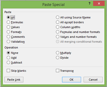
Tip: You can also select Home > Paste > Paste Special.
To pick an option in the dialog box, press the underlined letter for that option. For example, press the letter C to pick the Comments option.
|
To do this |
Press |
|---|---|
|
Paste all cell contents and formatting. |
A |
|
Paste only the formulas as entered in the formula bar. |
F |
|
Paste only the values (not the formulas). |
V |
|
Paste only the copied formatting. |
T |
|
Paste only comments and notes attached to the cell. |
C |
|
Paste only the data validation settings from copied cells. |
N |
|
Paste all cell contents and formatting from copied cells. |
H |
|
Paste all cell contents without borders. |
X |
|
Paste only column widths from copied cells. |
W |
|
Paste only formulas and number formats from copied cells. |
R |
|
Paste only the values (not formulas) and number formats from copied cells. |
U |
Top of Page
Keyboard shortcuts for making selections and performing actions
|
To do this |
Press |
|---|---|
|
Select the entire worksheet. |
Ctrl+A or Ctrl+Shift+Spacebar |
|
Select the current and next sheet in a workbook. |
Ctrl+Shift+Page down |
|
Select the current and previous sheet in a workbook. |
Ctrl+Shift+Page up |
|
Extend the selection of cells by one cell. |
Shift+Arrow key |
|
Extend the selection of cells to the last nonblank cell in the same column or row as the active cell, or if the next cell is blank, to the next nonblank cell. |
Ctrl+Shift+Arrow key |
|
Turn extend mode on and use the arrow keys to extend a selection. Press again to turn off. |
F8 |
|
Add a non-adjacent cell or range to a selection of cells by using the arrow keys. |
Shift+F8 |
|
Start a new line in the same cell. |
Alt+Enter |
|
Fill the selected cell range with the current entry. |
Ctrl+Enter |
|
Complete a cell entry and select the cell above. |
Shift+Enter |
|
Select an entire column in a worksheet. |
Ctrl+Spacebar |
|
Select an entire row in a worksheet. |
Shift+Spacebar |
|
Select all objects on a worksheet when an object is selected. |
Ctrl+Shift+Spacebar |
|
Extend the selection of cells to the beginning of the worksheet. |
Ctrl+Shift+Home |
|
Select the current region if the worksheet contains data. Press a second time to select the current region and its summary rows. Press a third time to select the entire worksheet. |
Ctrl+A or Ctrl+Shift+Spacebar |
|
Select the current region around the active cell. |
Ctrl+Shift+Asterisk sign (*) |
|
Select the first command on the menu when a menu or submenu is visible. |
Home |
|
Repeat the last command or action, if possible. |
Ctrl+Y |
|
Undo the last action. |
Ctrl+Z |
|
Expand grouped rows or columns. |
While hovering over the collapsed items, press and hold the Shift key and scroll down. |
|
Collapse grouped rows or columns. |
While hovering over the expanded items, press and hold the Shift key and scroll up. |
Top of Page
Keyboard shortcuts for working with data, functions, and the formula bar
|
To do this |
Press |
|---|---|
|
Turn on or off tooltips for checking formulas directly in the formula bar or in the cell you’re editing. |
Ctrl+Alt+P |
|
Edit the active cell and put the insertion point at the end of its contents. Or, if editing is turned off for the cell, move the insertion point into the formula bar. If editing a formula, toggle Point mode off or on so you can use the arrow keys to create a reference. |
F2 |
|
Expand or collapse the formula bar. |
Ctrl+Shift+U |
|
Cancel an entry in the cell or formula bar. |
Esc |
|
Complete an entry in the formula bar and select the cell below. |
Enter |
|
Move the cursor to the end of the text when in the formula bar. |
Ctrl+End |
|
Select all text in the formula bar from the cursor position to the end. |
Ctrl+Shift+End |
|
Calculate all worksheets in all open workbooks. |
F9 |
|
Calculate the active worksheet. |
Shift+F9 |
|
Calculate all worksheets in all open workbooks, regardless of whether they have changed since the last calculation. |
Ctrl+Alt+F9 |
|
Check dependent formulas, and then calculate all cells in all open workbooks, including cells not marked as needing to be calculated. |
Ctrl+Alt+Shift+F9 |
|
Display the menu or message for an Error Checking button. |
Alt+Shift+F10 |
|
Display the Function Arguments dialog box when the insertion point is to the right of a function name in a formula. |
Ctrl+A |
|
Insert argument names and parentheses when the insertion point is to the right of a function name in a formula. |
Ctrl+Shift+A |
|
Insert the AutoSum formula |
Alt+Equal sign ( = ) |
|
Invoke Flash Fill to automatically recognize patterns in adjacent columns and fill the current column |
Ctrl+E |
|
Cycle through all combinations of absolute and relative references in a formula if a cell reference or range is selected. |
F4 |
|
Insert a function. |
Shift+F3 |
|
Copy the value from the cell above the active cell into the cell or the formula bar. |
Ctrl+Shift+Straight quotation mark («) |
|
Create an embedded chart of the data in the current range. |
Alt+F1 |
|
Create a chart of the data in the current range in a separate Chart sheet. |
F11 |
|
Define a name to use in references. |
Alt+M, M, D |
|
Paste a name from the Paste Name dialog box (if names have been defined in the workbook). |
F3 |
|
Move to the first field in the next record of a data form. |
Enter |
|
Create, run, edit, or delete a macro. |
Alt+F8 |
|
Open the Microsoft Visual Basic For Applications Editor. |
Alt+F11 |
|
Open the Power Query Editor |
Alt+F12 |
Top of Page
Keyboard shortcuts for refreshing external data
Use the following keys to refresh data from external data sources.
|
To do this |
Press |
|---|---|
|
Stop a refresh operation. |
Esc |
|
Refresh data in the current worksheet. |
Ctrl+F5 |
|
Refresh all data in the workbook. |
Ctrl+Alt+F5 |
Top of Page
Power Pivot keyboard shortcuts
Use the following keyboard shortcuts with Power Pivot in Microsoft 365, Excel 2019, Excel 2016, and Excel 2013.
|
To do this |
Press |
|---|---|
|
Open the context menu for the selected cell, column, or row. |
Shift+F10 |
|
Select the entire table. |
Ctrl+A |
|
Copy selected data. |
Ctrl+C |
|
Delete the table. |
Ctrl+D |
|
Move the table. |
Ctrl+M |
|
Rename the table. |
Ctrl+R |
|
Save the file. |
Ctrl+S |
|
Redo the last action. |
Ctrl+Y |
|
Undo the last action. |
Ctrl+Z |
|
Select the current column. |
Ctrl+Spacebar |
|
Select the current row. |
Shift+Spacebar |
|
Select all cells from the current location to the last cell of the column. |
Shift+Page down |
|
Select all cells from the current location to the first cell of the column. |
Shift+Page up |
|
Select all cells from the current location to the last cell of the row. |
Shift+End |
|
Select all cells from the current location to the first cell of the row. |
Shift+Home |
|
Move to the previous table. |
Ctrl+Page up |
|
Move to the next table. |
Ctrl+Page down |
|
Move to the first cell in the upper-left corner of selected table. |
Ctrl+Home |
|
Move to the last cell in the lower-right corner of selected table. |
Ctrl+End |
|
Move to the first cell of the selected row. |
Ctrl+Left arrow key |
|
Move to the last cell of the selected row. |
Ctrl+Right arrow key |
|
Move to the first cell of the selected column. |
Ctrl+Up arrow key |
|
Move to the last cell of selected column. |
Ctrl+Down arrow key |
|
Close a dialog box or cancel a process, such as a paste operation. |
Ctrl+Esc |
|
Open the AutoFilter Menu dialog box. |
Alt+Down arrow key |
|
Open the Go To dialog box. |
F5 |
|
Recalculate all formulas in the Power Pivot window. For more information, see Recalculate Formulas in Power Pivot. |
F9 |
Top of Page
Function keys
|
Key |
Description |
|---|---|
|
F1 |
|
|
F2 |
|
|
F3 |
|
|
F4 |
|
|
F5 |
|
|
F6 |
|
|
F7 |
|
|
F8 |
|
|
F9 |
|
|
F10 |
|
|
F11 |
|
|
F12 |
|
Top of Page
Other useful shortcut keys
|
Key |
Description |
|---|---|
|
Alt |
For example,
|
|
Arrow keys |
|
|
Backspace |
|
|
Delete |
|
|
End |
|
|
Enter |
|
|
Esc |
|
|
Home |
|
|
Page down |
|
|
Page up |
|
|
Shift |
|
|
Spacebar |
|
|
Tab key |
|
Top of Page
See also
Excel help & learning
Basic tasks using a screen reader with Excel
Use a screen reader to explore and navigate Excel
Screen reader support for Excel
This article describes the keyboard shortcuts, function keys, and some other common shortcut keys in Excel for Mac.
Notes:
-
The settings in some versions of the Mac operating system (OS) and some utility applications might conflict with keyboard shortcuts and function key operations in Microsoft 365 for Mac.
-
If you don’t find a keyboard shortcut here that meets your needs, you can create a custom keyboard shortcut. For instructions, go to Create a custom keyboard shortcut for Office for Mac.
-
Many of the shortcuts that use the Ctrl key on a Windows keyboard also work with the Control key in Excel for Mac. However, not all do.
-
To quickly find a shortcut in this article, you can use the Search. Press
 +F, and then type your search words.
 -
Click-to-add is available but requires a setup. Select Excel> Preferences > Edit > Enable Click to Add Mode. To start a formula, type an equal sign ( = ), and then select cells to add them together. The plus sign (+) will be added automatically.
In this topic
-
Frequently used shortcuts
-
Shortcut conflicts
-
Change system preferences for keyboard shortcuts with the mouse
-
-
Work in windows and dialog boxes
-
Move and scroll in a sheet or workbook
-
Enter data on a sheet
-
Work in cells or the Formula bar
-
Format and edit data
-
Select cells, columns, or rows
-
Work with a selection
-
Use charts
-
Sort, filter, and use PivotTable reports
-
Outline data
-
Use function key shortcuts
-
Change function key preferences with the mouse
-
-
Drawing
Frequently used shortcuts
This table itemizes the most frequently used shortcuts in Excel for Mac.
|
To do this |
Press |
|---|---|
|
Paste selection. |
|
|
Copy selection. |
|
|
Clear selection. |
Delete |
|
Save workbook. |
|
|
Undo action. |
|
|
Redo action. |
|
|
Cut selection. |
|
|
Apply bold formatting. |
|
|
Print workbook. |
|
|
Open Visual Basic. |
Option+F11 |
|
Fill cells down. |
|
|
Fill cells right. |
|
|
Insert cells. |
Control+Shift+Equal sign ( = ) |
|
Delete cells. |
|
|
Calculate all open workbooks. |
|
|
Close window. |
|
|
Quit Excel. |
|
|
Display the Go To dialog box. |
Control+G |
|
Display the Format Cells dialog box. |
|
|
Display the Replace dialog box. |
Control+H |
|
Use Paste Special. |
|
|
Apply underline formatting. |
|
|
Apply italic formatting. |
|
|
Open a new blank workbook. |
|
|
Create a new workbook from template. |
|
|
Display the Save As dialog box. |
|
|
Display the Help window. |
F1 |
|
Select all. |
|
|
Add or remove a filter. |
|
|
Minimize or maximize the ribbon tabs. |
|
|
Display the Open dialog box. |
|
|
Check spelling. |
F7 |
|
Open the thesaurus. |
Shift+F7 |
|
Display the Formula Builder. |
Shift+F3 |
|
Open the Define Name dialog box. |
|
|
Insert or reply to a threaded comment. |
|
|
Open the Create names dialog box. |
|
|
Insert a new sheet. * |
Shift+F11 |
|
Print preview. |
|

Top of Page
Shortcut conflicts
Some Windows keyboard shortcuts conflict with the corresponding default macOS keyboard shortcuts. This topic flags such shortcuts with an asterisk (*). To use these shortcuts, you might have to change your Mac keyboard settings to change the Show Desktop shortcut for the key.
Change system preferences for keyboard shortcuts with the mouse
-
On the Apple menu, select System Settings.
-
Select Keyboard.
-
Select Keyboard Shortcuts.
-
Find the shortcut that you want to use in Excel and clear the checkbox for it.
Top of Page
Work in windows and dialog boxes
|
To do this |
Press |
|---|---|
|
Expand or minimize the ribbon. |
|
|
Switch to full screen view. |
|
|
Switch to the next application. |
|
|
Switch to the previous application. |
Shift+ |
|
Close the active workbook window. |
|
|
Take a screenshot and save it on your desktop. |
Shift+ |
|
Minimize the active window. |
Control+F9 |
|
Maximize or restore the active window. |
Control+F10 |
|
Hide Excel. |
|
|
Move to the next box, option, control, or command. |
Tab key |
|
Move to the previous box, option, control, or command. |
Shift+Tab |
|
Exit a dialog box or cancel an action. |
Esc |
|
Perform the action assigned to the default button (the button with the bold outline). |
Return |
|
Cancel the command and close the dialog box or menu. |
Esc |
Top of Page
Move and scroll in a sheet or workbook
|
To do this |
Press |
|---|---|
|
Move one cell up, down, left, or right. |
Arrow keys |
|
Move to the edge of the current data region. |
|
|
Move to the beginning of the row. |
Home |
|
Move to the beginning of the sheet. |
Control+Home |
|
Move to the last cell in use on the sheet. |
Control+End |
|
Move down one screen. |
Page down |
|
Move up one screen. |
Page up |
|
Move one screen to the right. |
Option+Page down |
|
Move one screen to the left. |
Option+Page up |
|
Move to the next sheet in the workbook. |
Control+Page down |
|
Move to the previous sheet in the workbook. |
Control+Page down |
|
Scroll to display the active cell. |
Control+Delete |
|
Display the Go To dialog box. |
Control+G |
|
Display the Find dialog box. |
Control+F |
|
Access search (when in a cell or when a cell is selected). |
|
|
Move between unlocked cells on a protected sheet. |
Tab key |
|
Scroll horizontally. |
Shift, then scroll the mouse wheel up for left, down for right |
Tip: To use the arrow keys to move between cells in Excel for Mac 2011, you must turn Scroll Lock off. To toggle Scroll Lock off or on, press Shift+F14. Depending on the type of your keyboard, you might need to use the Control, Option, or the Command key instead of the Shift key. If you are using a MacBook, you might need to plug in a USB keyboard to use the F14 key combination.
Top of Page
Enter data on a sheet
|
To do this |
Press |
|---|---|
|
Edit the selected cell. |
F2 |
|
Complete a cell entry and move forward in the selection. |
Return |
|
Start a new line in the same cell. |
Option+Return or Control+Option+Return |
|
Fill the selected cell range with the text that you type. |
|
|
Complete a cell entry and move up in the selection. |
Shift+Return |
|
Complete a cell entry and move to the right in the selection. |
Tab key |
|
Complete a cell entry and move to the left in the selection. |
Shift+Tab |
|
Cancel a cell entry. |
Esc |
|
Delete the character to the left of the insertion point or delete the selection. |
Delete |
|
Delete the character to the right of the insertion point or delete the selection. Note: Some smaller keyboards do not have this key. |
|
|
Delete text to the end of the line. Note: Some smaller keyboards do not have this key. |
Control+ |
|
Move one character up, down, left, or right. |
Arrow keys |
|
Move to the beginning of the line. |
Home |
|
Insert a note. |
Shift+F2 |
|
Open and edit a cell note. |
Shift+F2 |
|
Insert a threaded comment. |
|
|
Open and reply to a threaded comment. |
|
|
Fill down. |
Control+D |
|
Fill to the right. |
Control+R |
|
Invoke Flash Fill to automatically recognize patterns in adjacent columns and fill the current column. |
Control+E |
|
Define a name. |
Control+L |
Top of Page
Work in cells or the Formula bar
|
To do this |
Press |
|---|---|
|
Turn on or off tooltips for checking formulas directly in the formula bar. |
Control+Option+P |
|
Edit the selected cell. |
F2 |
|
Expand or collapse the formula bar. |
Control+Shift+U |
|
Edit the active cell and then clear it or delete the preceding character in the active cell as you edit the cell contents. |
Delete |
|
Complete a cell entry. |
Return |
|
Enter a formula as an array formula. |
Shift+ |
|
Cancel an entry in the cell or formula bar. |
Esc |
|
Display the Formula Builder after you type a valid function name in a formula |
Control+A |
|
Insert a hyperlink. |
|
|
Edit the active cell and position the insertion point at the end of the line. |
Control+U |
|
Open the Formula Builder. |
Shift+F3 |
|
Calculate the active sheet. |
Shift+F9 |
|
Display the context menu. |
Shift+F10 |
|
Start a formula. |
Equal sign ( = ) |
|
Toggle the formula reference style between absolute, relative, and mixed. |
|
|
Insert the AutoSum formula. |
Shift+ |
|
Enter the date. |
Control+Semicolon (;) |
|
Enter the time. |
|
|
Copy the value from the cell above the active cell into the cell or the formula bar. |
Control+Shift+Inch mark/Straight double quote («) |
|
Alternate between displaying cell values and displaying cell formulas. |
Control+Grave accent (`) |
|
Copy a formula from the cell above the active cell into the cell or the formula bar. |
Control+Apostrophe (‘) |
|
Display the AutoComplete list. |
Option+Down arrow key |
|
Define a name. |
Control+L |
|
Open the Smart Lookup pane. |
Control+Option+ |
Top of Page
Format and edit data
|
To do this |
Press |
|---|---|
|
Edit the selected cell. |
F2 |
|
Create a table. |
|
|
Insert a line break in a cell. |
|
|
Insert special characters like symbols, including emoji. |
Control+ |
|
Increase font size. |
Shift+ |
|
Decrease font size. |
Shift+ |
|
Align center. |
|
|
Align left. |
|
|
Display the Modify Cell Style dialog box. |
Shift+ |
|
Display the Format Cells dialog box. |
|
|
Apply the general number format. |
Control+Shift+Tilde (~) |
|
Apply the currency format with two decimal places (negative numbers appear in red with parentheses). |
Control+Shift+Dollar sign ($) |
|
Apply the percentage format with no decimal places. |
Control+Shift+Percent sign (%) |
|
Apply the exponential number format with two decimal places. |
Control+Shift+Caret (^) |
|
Apply the date format with the day, month, and year. |
Control+Shift+Number sign (#) |
|
Apply the time format with the hour and minute, and indicate AM or PM. |
Control+Shift+At symbol (@) |
|
Apply the number format with two decimal places, thousands separator, and minus sign (-) for negative values. |
Control+Shift+Exclamation point (!) |
|
Apply the outline border around the selected cells. |
|
|
Add an outline border to the right of the selection. |
|
|
Add an outline border to the left of the selection. |
|
|
Add an outline border to the top of the selection. |
|
|
Add an outline border to the bottom of the selection. |
|
|
Remove outline borders. |
|
|
Apply or remove bold formatting. |
|
|
Apply or remove italic formatting. |
|
|
Apply or remove underline formatting. |
|
|
Apply or remove strikethrough formatting. |
Shift+ |
|
Hide a column. |
|
|
Unhide a column. |
Shift+ |
|
Hide a row. |
|
|
Unhide a row. |
Shift+ |
|
Edit the active cell. |
Control+U |
|
Cancel an entry in the cell or the formula bar. |
Esc |
|
Edit the active cell and then clear it or delete the preceding character in the active cell as you edit the cell contents. |
Delete |
|
Paste text into the active cell. |
|
|
Complete a cell entry |
Return |
|
Give selected cells the current cell’s entry. |
|
|
Enter a formula as an array formula. |
Shift+ |
|
Display the Formula Builder after you type a valid function name in a formula. |
Control+A |
Top of Page
Select cells, columns, or rows
|
To do this |
Press |
|---|---|
|
Extend the selection by one cell. |
Shift+Arrow key |
|
Extend the selection to the last nonblank cell in the same column or row as the active cell. |
Shift+ |
|
Extend the selection to the beginning of the row. |
Shift+Home |
|
Extend the selection to the beginning of the sheet. |
Control+Shift+Home |
|
Extend the selection to the last cell used |
Control+Shift+End |
|
Select the entire column. * |
Control+Spacebar |
|
Select the entire row. |
Shift+Spacebar |
|
Select the current region or entire sheet. Press more than once to expand the selection. |
|
|
Select only visible cells. |
Shift+ |
|
Select only the active cell when multiple cells are selected. |
Shift+Delete |
|
Extend the selection down one screen. |
Shift+Page down |
|
Extend the selection up one screen |
Shift+Page up |
|
Alternate between hiding objects, displaying objects, |
Control+6 |
|
Turn on the capability to extend a selection |
F8 |
|
Add another range of cells to the selection. |
Shift+F8 |
|
Select the current array, which is the array that the |
Control+Forward slash (/) |
|
Select cells in a row that don’t match the value |
Control+Backward slash () |
|
Select only cells that are directly referred to by formulas in the selection. |
Control+Shift+Left bracket ([) |
|
Select all cells that are directly or indirectly referred to by formulas in the selection. |
Control+Shift+Left brace ({) |
|
Select only cells with formulas that refer directly to the active cell. |
Control+Right bracket (]) |
|
Select all cells with formulas that refer directly or indirectly to the active cell. |
Control+Shift+Right brace (}) |
Top of Page
Work with a selection
|
To do this |
Press |
|---|---|
|
Copy a selection. |
|
|
Paste a selection. |
|
|
Cut a selection. |
|
|
Clear a selection. |
Delete |
|
Delete the selection. |
Control+Hyphen |
|
Undo the last action. |
|
|
Hide a column. |
|
|
Unhide a column. |
|
|
Hide a row. |
|
|
Unhide a row. |
|
|
Move selected rows, columns, or cells. |
Hold the Shift key while you drag a selected row, column, or selected cells to move the selected cells and drop to insert them in a new location. If you don’t hold the Shift key while you drag and drop, the selected cells will be cut from the original location and pasted to the new location (not inserted). |
|
Move from top to bottom within the selection (down). * |
Return |
|
Move from bottom to top within the selection (up). * |
Shift+Return |
|
Move from left to right within the selection, |
Tab key |
|
Move from right to left within the selection, |
Shift+Tab |
|
Move clockwise to the next corner of the selection. |
Control+Period (.) |
|
Group selected cells. |
|
|
Ungroup selected cells. |
|
* These shortcuts might move in another direction other than down or up. If you’d like to change the direction of these shortcuts using the mouse, select Excel > Preferences > Edit, and then, in After pressing Return, move selection, select the direction you want to move to.
Top of Page
Use charts
|
To do this |
Press |
|---|---|
|
Insert a new chart sheet. * |
F11 |
|
Cycle through chart object selection. |
Arrow keys |
Top of Page
Sort, filter, and use PivotTable reports
|
To do this |
Press |
|---|---|
|
Open the Sort dialog box. |
|
|
Add or remove a filter. |
|
|
Display the Filter list or PivotTable page |
Option+Down arrow key |
Top of Page
Outline data
|
To do this |
Press |
|---|---|
|
Display or hide outline symbols. |
Control+8 |
|
Hide selected rows. |
Control+9 |
|
Unhide selected rows. |
Control+Shift+Left parenthesis (() |
|
Hide selected columns. |
Control+Zero (0) |
|
Unhide selected columns. |
Control+Shift+Right parenthesis ()) |
Top of Page
Use function key shortcuts
Excel for Mac uses the function keys for common commands, including Copy and Paste. For quick access to these shortcuts, you can change your Apple system preferences, so you don’t have to press the Fn key every time you use a function key shortcut.
Note: Changing system function key preferences affects how the function keys work for your Mac, not just Excel for Mac. After changing this setting, you can still perform the special features printed on a function key. Just press the Fn key. For example, to use the F12 key to change your volume, you would press Fn+F12.
If a function key doesn’t work as you expect it to, press the Fn key in addition to the function key. If you don’t want to press the Fn key each time, you can change your Apple system preferences. For instructions, go to Change function key preferences with the mouse.
The following table provides the function key shortcuts for Excel for Mac.
|
To do this |
Press |
|---|---|
|
Display the Help window. |
F1 |
|
Edit the selected cell. |
F2 |
|
Insert a note or open and edit a cell note. |
Shift+F2 |
|
Insert a threaded comment or open and reply to a threaded comment. |
|
|
Open the Save dialog box. |
Option+F2 |
|
Open the Formula Builder. |
Shift+F3 |
|
Open the Define Name dialog box. |
|
|
Close a window or a dialog box. |
|
|
Display the Go To dialog box. |
F5 |
|
Display the Find dialog box. |
Shift+F5 |
|
Move to the Search Sheet dialog box. |
Control+F5 |
|
Switch focus between the worksheet, ribbon, task pane, and status bar. |
F6 or Shift+F6 |
|
Check spelling. |
F7 |
|
Open the thesaurus. |
Shift+F7 |
|
Extend the selection. |
F8 |
|
Add to the selection. |
Shift+F8 |
|
Display the Macro dialog box. |
Option+F8 |
|
Calculate all open workbooks. |
F9 |
|
Calculate the active sheet. |
Shift+F9 |
|
Minimize the active window. |
Control+F9 |
|
Display the context menu, or «right click» menu. |
Shift+F10 |
|
Display a pop-up menu (on object button menu), such as by clicking the button after you paste into a sheet. |
Option+Shift+F10 |
|
Maximize or restore the active window. |
Control+F10 |
|
Insert a new chart sheet.* |
F11 |
|
Insert a new sheet.* |
Shift+F11 |
|
Insert an Excel 4.0 macro sheet. |
|
|
Open Visual Basic. |
Option+F11 |
|
Display the Save As dialog box. |
F12 |
|
Display the Open dialog box. |
|
|
Open the Power Query Editor |
Option+F12 |
Top of Page
Change function key preferences with the mouse
-
On the Apple menu, select System Preferences > Keyboard.
-
On the Keyboard tab, select the checkbox for Use all F1, F2, etc. keys as standard function keys.
Drawing
|
To do this |
Press |
|---|---|
|
Toggle Drawing mode on and off. |
|
Top of Page
See also
Excel help & learning
Use a screen reader to explore and navigate Excel
Basic tasks using a screen reader with Excel
Screen reader support for Excel
This article describes the keyboard shortcuts in Excel for iOS.
Notes:
-
If you’re familiar with keyboard shortcuts on your macOS computer, the same key combinations work with Excel for iOS using an external keyboard, too.
-
To quickly find a shortcut, you can use the Search. Press
+F and then type your search words.
In this topic
-
Navigate the worksheet
-
Format and edit data
-
Work in cells or the formula bar
Navigate the worksheet
|
To do this |
Press |
|---|---|
|
Move one cell to the right. |
Tab key |
|
Move one cell up, down, left, or right. |
Arrow keys |
|
Move to the next sheet in the workbook. |
Option+Right arrow key |
|
Move to the previous sheet in the workbook. |
Option+Left arrow key |
Top of Page
Format and edit data
|
To do this |
Press |
|---|---|
|
Apply outline border. |
|
|
Remove outline border. |
|
|
Hide column(s). |
|
|
Hide row(s). |
Control+9 |
|
Unhide column(s). |
Shift+ |
|
Unhide row(s). |
Shift+Control+9 or Shift+Control+Left parenthesis (() |
Top of Page
Work in cells or the formula bar
|
To do this |
Press |
|---|---|
|
Move to the cell on the right. |
Tab key |
|
Move within cell text. |
Arrow keys |
|
Copy a selection. |
|
|
Paste a selection. |
|
|
Cut a selection. |
|
|
Undo an action. |
|
|
Redo an action. |
|
|
Apply bold formatting to the selected text. |
|
|
Apply italic formatting to the selected text. |
|
|
Underline the selected text. |
|
|
Select all. |
|
|
Select a range of cells. |
Shift+Left or Right arrow key |
|
Insert a line break within a cell. |
|
|
Move the cursor to the beginning of the current line within a cell. |
|
|
Move the cursor to the end of the current line within a cell. |
|
|
Move the cursor to the beginning of the current cell. |
|
|
Move the cursor to the end of the current cell. |
|
|
Move the cursor up by one paragraph within a cell that contains a line break. |
Option+Up arrow key |
|
Move the cursor down by one paragraph within a cell that contains a line break. |
Option+Down arrow key |
|
Move the cursor right by one word. |
Option+Right arrow key |
|
Move the cursor left by one word. |
Option+Left arrow key |
|
Insert an AutoSum formula. |
Shift+ |
Top of Page
See also
Excel help & learning
Screen reader support for Excel
Basic tasks using a screen reader with Excel
Use a screen reader to explore and navigate Excel
This article describes the keyboard shortcuts in Excel for Android.
Notes:
-
If you’re familiar with keyboard shortcuts on your Windows computer, the same key combinations work with Excel for Android using an external keyboard, too.
-
To quickly find a shortcut, you can use the Search. Press Control+F and then type your search words.
In this topic
-
Navigate the worksheet
-
Work with cells
Navigate the worksheet
|
To do this |
Press |
|---|---|
|
Move one cell to the right. |
Tab key |
|
Move one cell up, down, left, or right. |
Up, Down, Left, or Right arrow key |
Top of Page
Work with cells
|
To do this |
Press |
|---|---|
|
Save a worksheet. |
Control+S |
|
Copy a selection. |
Control+C |
|
Paste a selection. |
Control+V |
|
Cut a selection. |
Control+X |
|
Undo an action. |
Control+Z |
|
Redo an action. |
Control+Y |
|
Apply bold formatting. |
Control+B |
|
Apply italic formatting. |
Control+I |
|
Apply underline formatting. |
Control+U |
|
Select all. |
Control+A |
|
Find. |
Control+F |
|
Insert a line break within a cell. |
Alt+Enter |
Top of Page
See also
Excel help & learning
Screen reader support for Excel
Basic tasks using a screen reader with Excel
Use a screen reader to explore and navigate Excel
This article describes the keyboard shortcuts in Excel for the web.
Notes:
-
If you use Narrator with the Windows 10 Fall Creators Update, you have to turn off scan mode in order to edit documents, spreadsheets, or presentations with Microsoft 365 for the web. For more information, refer to Turn off virtual or browse mode in screen readers in Windows 10 Fall Creators Update.
-
To quickly find a shortcut, you can use the Search. Press Ctrl+F and then type your search words.
-
When you use Excel for the web, we recommend that you use Microsoft Edge as your web browser. Because Excel for the web runs in your web browser, the keyboard shortcuts are different from those in the desktop program. For example, you’ll use Ctrl+F6 instead of F6 for jumping in and out of the commands. Also, common shortcuts like F1 (Help) and Ctrl+O (Open) apply to the web browser — not Excel for the web.
In this article
-
Quick tips for using keyboard shortcuts with Excel for the web
-
Frequently used shortcuts
-
Access keys: Shortcuts for using the ribbon
-
Keyboard shortcuts for editing cells
-
Keyboard shortcuts for entering data
-
Keyboard shortcuts for editing data within a cell
-
Keyboard shortcuts for formatting cells
-
Keyboard shortcuts for moving and scrolling within worksheets
-
Keyboard shortcuts for working with objects
-
Keyboard shortcuts for working with cells, rows, columns, and objects
-
Keyboard shortcuts for moving within a selected range
-
Keyboard shortcuts for calculating data
-
Accessibility Shortcuts Menu (Alt+Shift+A)
-
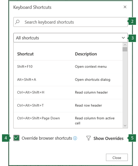
Control keyboard shortcuts in Excel for the web by overriding browser keyboard shortcuts
Quick tips for using keyboard shortcuts with Excel for the web
-
To find any command quickly, press Alt+Windows logo key, Q to jump to the Search or Tell Me text field. In Search or Tell Me, type a word or the name of a command you want (available only in Editing mode). Search or Tell Me searches for related options and provides a list. Use the Up and Down arrow keys to select a command, and then press Enter.
Depending on the version of Microsoft 365 you are using, the Search text field at the top of the app window might be called Tell Me instead. Both offer a largely similar experience, but some options and search results can vary.
-
To jump to a particular cell in a workbook, use the Go To option: press Ctrl+G, type the cell reference (such as B14), and then press Enter.
-
If you use a screen reader, go to Accessibility Shortcuts Menu (Alt+Shift+A).
Frequently used shortcuts
These are the most frequently used shortcuts for Excel for the web.
Tip: To quickly create a new worksheet in Excel for the web, open your browser, type Excel.new in the address bar, and then press Enter.
|
To do this |
Press |
|---|---|
|
Go to a specific cell. |
Ctrl+G |
|
Move down. |
Page down or Down arrow key |
|
Move up. |
Page up or Up arrow key |
|
Print a workbook. |
Ctrl+P |
|
Copy selection. |
Ctrl+C |
|
Paste selection. |
Ctrl+V |
|
Cut selection. |
Ctrl+X |
|
Undo action. |
Ctrl+Z |
|
Open workbook. |
Ctrl+O |
|
Close workbook. |
Ctrl+W |
|
Open the Save As dialog box. |
Alt+F2 |
|
Use Find. |
Ctrl+F or Shift+F3 |
|
Apply bold formatting. |
Ctrl+B |
|
Open the context menu. |
|
|
Jump to Search or Tell me. |
Alt+Q |
|
Repeat Find downward. |
Shift+F4 |
|
Repeat Find upward. |
Ctrl+Shift+F4 |
|
Insert a chart. |
Alt+F1 |
|
Display the access keys (ribbon commands) on the classic ribbon when using Narrator. |
Alt+Period (.) |
Top of Page
Access keys: Shortcuts for using the ribbon
Excel for the web offers access keys, keyboard shortcuts to navigate the ribbon. If you’ve used access keys to save time on Excel for desktop computers, you’ll find access keys very similar in Excel for the web.
In Excel for the web, access keys all start with Alt+Windows logo key, then add a letter for the ribbon tab. For example, to go to the Review tab, press Alt+Windows logo key, R.
Note: To learn how to override the browser’s Alt-based ribbon shortcuts, go to Control keyboard shortcuts in Excel for the web by overriding browser keyboard shortcuts.
If you’re using Excel for the web on a Mac computer, press Control+Option to start.
-
To get to the ribbon, press Alt+Windows logo key, or press Ctrl+F6 until you reach the Home tab.
-
To move between tabs on the ribbon, press the Tab key.
-
To hide the ribbon so you have more room to work, press Ctrl+F1. To display the ribbon again, press Ctrl+F1.
Go to the access keys for the ribbon
To go directly to a tab on the ribbon, press one of the following access keys:
|
To do this |
Press |
|---|---|
|
Go to the Search or Tell Me field on the ribbon and type a search term. |
Alt+Windows logo key, Q |
|
Open the File menu. |
Alt+Windows logo key, F |
|
Open the Home tab and format text and numbers or use other tools such as Sort & Filter. |
Alt+Windows logo key, H |
|
Open the Insert tab and insert a function, table, chart, hyperlink, or threaded comment. |
Alt+Windows logo key, N |
|
Open the Data tab and refresh connections or use data tools. |
Alt+Windows logo key, A |
|
Open the Review tab and use the Accessibility Checker or work with threaded comments and notes. |
Alt+Windows logo key, R |
|
Open the View tab to choose a view, freeze rows or columns in your worksheet, or show gridlines and headers. |
Alt+Windows logo key, W |
Top of Page
Work in the ribbon tabs and menus
The shortcuts in this table can save time when you work with the ribbon tabs and ribbon menus.
|
To do this |
Press |
|---|---|
|
Select the active tab of the ribbon and activate the access keys. |
Alt+Windows logo key. To move to a different tab, use an access key or the Tab key. |
|
Move the focus to commands on the ribbon. |
Enter, then the Tab key or Shift+Tab |
|
Activate a selected button. |
Spacebar or Enter |
|
Open the list for a selected command. |
Spacebar or Enter |
|
Open the menu for a selected button. |
Alt+Down arrow key |
|
When a menu or submenu is open, move to the next command. |
Esc |
Top of Page
Keyboard shortcuts for editing cells
Tip: If a spreadsheet opens in the Viewing mode, editing commands won’t work. To switch to Editing mode, press Alt+Windows logo key, Z, M, E.
|
To do this |
Press |
|---|---|
|
Insert a row above the current row. |
Alt+Windows logo key, H, I, R |
|
Insert a column to the left of the current column. |
Alt+Windows logo key, H, I, C |
|
Cut selection. |
Ctrl+X |
|
Copy selection. |
Ctrl+C |
|
Paste selection. |
Ctrl+V |
|
Undo an action. |
Ctrl+Z |
|
Redo an action. |
Ctrl+Y |
|
Start a new line in the same cell. |
Alt+Enter |
|
Insert a hyperlink. |
Ctrl+K |
|
Insert a table. |
Ctrl+L |
|
Insert a function. |
Shift+F3 |
|
Increase font size. |
Ctrl+Shift+Right angle bracket (>) |
|
Decrease font size. |
Ctrl+Shift+Left angle bracket (<) |
|
Apply a filter. |
Alt+Windows logo key, A, T |
|
Re-apply a filter. |
Ctrl+Alt+L |
|
Toggle AutoFilter on and off. |
Ctrl+Shift+L |
Top of Page
Keyboard shortcuts for entering data
|
To do this |
Press |
|---|---|
|
Complete cell entry and select the cell below. |
Enter |
|
Complete cell entry and select the cell above. |
Shift+Enter |
|
Complete cell entry and select the next cell in the row. |
Tab key |
|
Complete cell entry and select the previous cell in the row. |
Shift+Tab |
|
Cancel cell entry. |
Esc |
Top of Page
Keyboard shortcuts for editing data within a cell
|
To do this |
Press |
|---|---|
|
Edit the selected cell. |
F2 |
|
Cycle through all the various combinations of absolute and relative references when a cell reference or range is selected in a formula. |
F4 |
|
Clear the selected cell. |
Delete |
|
Clear the selected cell and start editing. |
Backspace |
|
Go to beginning of cell line. |
Home |
|
Go to end of cell line. |
End |
|
Select right by one character. |
Shift+Right arrow key |
|
Select to the beginning of cell data. |
Shift+Home |
|
Select to the end of cell data. |
Shift+End |
|
Select left by one character. |
Shift+Left arrow key |
|
Extend selection to the last nonblank cell in the same column or row as the active cell, or if the next cell is blank, to the next nonblank cell. |
Ctrl+Shift+Right arrow key or Ctrl+Shift+Left arrow key |
|
Insert the current date. |
Ctrl+Semicolon (;) |
|
Insert the current time. |
Ctrl+Shift+Semicolon (;) |
|
Copy a formula from the cell above. |
Ctrl+Apostrophe (‘) |
|
Copy the value from the cell above. |
Ctrl+Shift+Apostrophe (‘) |
|
Insert a formula argument. |
Ctrl+Shift+A |
Top of Page
Keyboard shortcuts for formatting cells
|
To do this |
Press |
|---|---|
|
Apply bold formatting. |
Ctrl+B |
|
Apply italic formatting. |
Ctrl+I |
|
Apply underline formatting. |
Ctrl+U |
|
Paste formatting. |
Shift+Ctrl+V |
|
Apply the outline border to the selected cells. |
Ctrl+Shift+Ampersand (&) |
|
Apply the number format. |
Ctrl+Shift+1 |
|
Apply the time format. |
Ctrl+Shift+2 |
|
Apply the date format. |
Ctrl+Shift+3 |
|
Apply the currency format. |
Ctrl+Shift+4 |
|
Apply the percentage format. |
Ctrl+Shift+5 |
|
Apply the scientific format. |
Ctrl+Shift+6 |
|
Apply outside border. |
Ctrl+Shift+7 |
|
Open the Number Format dialog box. |
Ctrl+1 |
Top of Page
Keyboard shortcuts for moving and scrolling within worksheets
|
To do this |
Press |
|---|---|
|
Move up one cell. |
Up arrow key or Shift+Enter |
|
Move down one cell. |
Down arrow key or Enter |
|
Move right one cell. |
Right arrow key or Tab key |
|
Go to the beginning of the row. |
Home |
|
Go to cell A1. |
Ctrl+Home |
|
Go to the last cell of the used range. |
Ctrl+End |
|
Move down one screen (28 rows). |
Page down |
|
Move up one screen (28 rows). |
Page up |
|
Move to the edge of the current data region. |
Ctrl+Right arrow key or Ctrl+Left arrow key |
|
Move between ribbon and workbook content. |
Ctrl+F6 |
|
Move to a different ribbon tab. |
Tab key Press Enter to go to the ribbon for the tab. |
|
Insert a new sheet. |
Shift+F11 |
|
Switch to the next sheet. |
Alt+Ctrl+Page down |
|
Switch to the next sheet (when in Microsoft Teams or a browser other than Chrome). |
Ctrl+Page down |
|
Switch to the previous sheet. |
Alt+Ctrl+Page up |
|
Switch to previous sheet (when in Microsoft Teams or a browser other than Chrome). |
Ctrl+Page up |
Top of Page
Keyboard shortcuts for working with objects
|
To do this |
Press |
|---|---|
|
Open menu or drill down. |
Alt+Down arrow key |
|
Close menu or drill up. |
Alt+Up arrow key |
|
Follow hyperlink. |
Ctrl+Enter |
|
Open a note for editing. |
Shift+F2 |
|
Open and reply to a threaded comment. |
Ctrl+Shift+F2 |
|
Rotate an object left. |
Alt+Left arrow key |
|
Rotate an object right. |
Alt+Right arrow key |
Top of Page
Keyboard shortcuts for working with cells, rows, columns, and objects
|
To do this |
Press |
|---|---|
|
Select a range of cells. |
Shift+Arrow keys |
|
Select an entire column. |
Ctrl+Spacebar |
|
Select an entire row. |
Shift+Spacebar |
|
Extend selection to the last nonblank cell in the same column or row as the active cell, or if the next cell is blank, to the next nonblank cell. |
Ctrl+Shift+Right arrow key or Ctrl+Shift+Left arrow key |
|
Add a non-adjacent cell or range to a selection. |
Shift+F8 |
|
Insert cells, rows, or columns. |
Ctrl+Plus sign (+) |
|
Delete cells, rows, or columns. |
Ctrl+Minus sign (-) |
|
Hide rows. |
Ctrl+9 |
|
Unhide rows. |
Ctrl+Shift+9 |
|
Hide columns |
Ctrl+0 |
|
Unhide columns |
Ctrl+Shift+0 |
Top of Page
Keyboard shortcuts for moving within a selected range
|
To do this |
Press |
|---|---|
|
Move from top to bottom (or forward through the selection). |
Enter |
|
Move from bottom to top (or back through the selection). |
Shift+Enter |
|
Move forward through a row (or down through a single-column selection). |
Tab key |
|
Move back through a row (or up through a single-column selection). |
Shift+Tab |
|
Move to an active cell. |
Shift+Backspace |
|
Move to an active cell and keep the selection. |
Ctrl+Backspace |
|
Rotate the active cell through the corners of the selection. |
Ctrl+Period (.) |
|
Move to the next selected range. |
Ctrl+Alt+Right arrow key |
|
Move to the previous selected range. |
Ctrl+Alt+Left arrow key |
|
Extend selection to the last used cell in the sheet. |
Ctrl+Shift+End |
|
Extend selection to the first cell in the sheet. |
Ctrl+Shift+Home |
Top of Page
Keyboard shortcuts for calculating data
|
To do this |
Press |
|---|---|
|
Calculate workbook (refresh). |
F9 |
|
Perform full calculation. |
Ctrl+Shift+Alt+F9 |
|
Refresh external data. |
Alt+F5 |
|
Refresh all external data. |
Ctrl+Alt+F5 |
|
Apply Auto Sum. |
Alt+Equal sign ( = ) |
|
Apply Flash Fill. |
Ctrl+E |
Top of Page
Accessibility Shortcuts Menu (Alt+Shift+A)
Access the common features quickly by using the following shortcuts:
|
To do this |
Press |
|---|---|
|
Cycle between landmark regions. |
Ctrl+F6 or Ctrl+Shift+F6 |
|
Move within a landmark region. |
Tab key or Shift+Tab |
|
Go to the Search or Tell Me field to run any command. |
Alt+Q |
|
Display or hide Key Tips or access the ribbon. |
Alt+Windows logo key |
|
Edit the selected cell. |
F2 |
|
Go to a specific cell. |
Ctrl+G |
|
Move to another worksheet in the workbook. |
Ctrl+Alt+Page up or Ctrl+Alt+Page down |
|
Open the context menu. |
Shift+F10 or Windows Menu key |
|
Read row header. |
Ctrl+Alt+Shift+T |
|
Read row until an active cell. |
Ctrl+Alt+Shift+Home |
|
Read row from an active cell. |
Ctrl+Alt+Shift+End |
|
Read column header. |
Ctrl+Alt+Shift+H |
|
Read column until an active cell. |
Ctrl+Alt+Shift+Page up |
|
Read column from an active cell. |
Ctrl+Alt+Shift+Page down |
|
Open a list of moving options within a dialog box. |
Ctrl+Alt+Spacebar |
Top of Page
Control keyboard shortcuts in Excel for the web by overriding browser keyboard shortcuts
Excel for the web works in a browser. Browsers have keyboard shortcuts, some of which conflict with shortcuts that work in Excel on the desktop. You can control these shortcuts, so they work the same in both versions of Excel by changing the Keyboard Shortcuts settings. Overriding browser shortcuts also enables you to open the Excel for the web Help by pressing F1.
|
|
Top of Page
See also
Excel help & learning
Use a screen reader to explore and navigate Excel
Basic tasks using a screen reader with Excel
Screen reader support for Excel
Technical support for customers with disabilities
Microsoft wants to provide the best possible experience for all our customers. If you have a disability or questions related to accessibility, please contact the Microsoft Disability Answer Desk for technical assistance. The Disability Answer Desk support team is trained in using many popular assistive technologies and can offer assistance in English, Spanish, French, and American Sign Language. Please go to the Microsoft Disability Answer Desk site to find out the contact details for your region.
If you are a government, commercial, or enterprise user, please contact the enterprise Disability Answer Desk.
Содержание
- Create a custom keyboard shortcut for Office for Mac
- Create Keyboard Shortcuts for your Favorite Excel Commands
- QAT Shortcuts
- QAT Customization
- Customize keyboard shortcuts
- Use a mouse to assign or remove a keyboard shortcut
- Use just the keyboard to assign or remove a keyboard shortcut
- Keyboard Shortcuts in Excel
- What are Excel Shortcuts?
- Top 20 Keyboard Shortcuts in Excel
- #1–Paste as Values With “Paste Special”
- #2–Sum Numbers With AutoSum
- #3–Fill the Subsequent Cell With the Fill Down
- #4–Select the Entire Row or Column
- #5–Insert and Delete Row or Column
- #6–Insert and Edit Comment
- #7–Move Between Sheets
- #8–Add Filters
- #9–Freeze Rows and Columns
- #10–Open “Format Cells” Dialog Box
- #11–Adjust Column Width
- #12–Repeat the Last Task
- #13–Insert Line Breaks in a Cell
- #14–Move Between Different Workbooks
- #15–Spell-Check
- #16–Move Between Worksheet and Excel VBA Editor
- #17–Select a Cell Range
- #18–Select the Last Non-Blank Cell of a Row or Column
- #19–Delete the Active Sheet
- #20–Insert a New Sheet
- Frequently Asked Questions
- Recommended Articles
- Comments
Create a custom keyboard shortcut for Office for Mac
You can create your own keyboard shortcuts in Microsoft 365 for Mac using the steps in this article.
You can create custom keyboard shortcuts in Excel or Word for Mac within the application itself. To create custom keyboard shortcuts in PowerPoint, Outlook, or OneNote for Mac, you can use the built-in capability in Mac OS X.
On the Tools menu, click Customize Keyboard.
In the Categories list, click a tab name.
In the Commands list, click the command that you want to assign a keyboard shortcut to.
Any keyboard shortcuts that are currently assigned to the selected command will appear in the Current keys box.
Tip: If you prefer to use a different keyboard shortcut, add another shortcut to the list, and then use it instead.
In the Press new keyboard shortcut box, type a key combination that includes at least one modifier key (  , CONTROL , OPTION , SHIFT ) and an additional key, such as + F11 .
If you type a keyboard shortcut that is already assigned, the action assigned to that key combination appears next to Currently assigned to.
Note: Keyboard shortcut descriptions refer to the U.S. keyboard layout. Keys on other keyboard layouts might not correspond to the keys on a U.S. keyboard. Keyboard shortcuts for laptop computers might also differ.
You can delete keyboard shortcuts that you created, but you cannot delete the default keyboard shortcuts for Excel.
On the Tools menu, click Customize Keyboard.
In the Categories list, click a tab name.
In the Commands list, click the command that you want to delete a keyboard shortcut from.
In the Current keys box, click the keyboard shortcut that you want to delete, and then click Remove.
Note: If the Remove button appears grayed out, then the selected keyboard shortcut is a default keyboard shortcut, and therefore it cannot be deleted.
On the Tools menu, click Customize Keyboard.
To restore keyboard shortcuts to their original state, click Reset All.
From the Apple menu, click System Preferences > Keyboard > Shortcuts > App Shortcuts.
Click the + sign to add a keyboard shortcut.
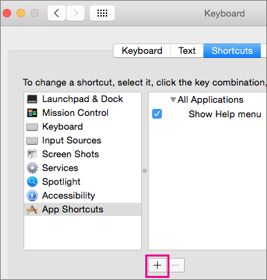
In the Application menu, click the Office for Mac app ( Microsoft Word, Microsoft PowerPoint, Microsoft OneNote, Microsoft Outlook) you want to create keyboard a shortcut for.
Enter a Menu Title and the Keyboard Shortcut and click Add.
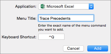
Tip: If you aren’t sure what the menu name is for a command, click Help in that app and search for what you want, which will then show you the exact menu name.
Источник
Create Keyboard Shortcuts for your Favorite Excel Commands
Generally, you can improve your speed by keeping your hands on your keyboard. But, what do you do if there is no built-in keyboard shortcut to execute your favorite command? Well, one approach is to customize the QAT. This post discusses the Quick Access Toolbar and the related keyboard shortcuts it creates.
QAT Shortcuts
Microsoft introduced the Quick Access Toolbar (QAT) in Excel 2007 with the rollout of the ribbon. It is a tiny little toolbar that includes a few commands by default, such as save, undo, and redo.
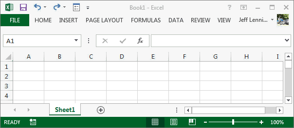
You can see it in the following screenshot just above the ribbon:

The nice thing about the QAT is that Excel automatically creates a simple keyboard shortcut to access its command icons. If you tap the Alt key, you’ll notice that the QAT icons each get a sequential number, 1, 2, 3, and so on, as shown below.
The QAT commands are easily accessed by tapping the corresponding Alt+Number combination. This is quite handy, especially since we can customize the QAT to include additional commands.
QAT Customization
Microsoft allows us to customize the QAT, including positioning it above or below the ribbon and adding/removing commands. On the right side of the QAT you’ll see a little dropdown arrow, and when you click it, you’ll have access to the various customization options, as shown below.
Some of the basic commands are provided in the dropdown menu, and you can toggle them on or off. In addition, you can select More Commands to open up the Excel Options dialog to select from a huge number of Excel commands. Remember how the QAT automatically creates an Alt shortcut for its icons? Well, when you add a command to the QAT you’ll be able to access it with a simple Alt shortcut. So, any frequently used commands become a simple shortcut away.
Let’s walk through an example. Back in Excel 2003 and earlier, I could quickly access the document properties dialog box by hitting Alt+F, I. I loved this dialog because it showed the full path of the file and I was able to quickly confirm that I was working on the correct document. I lost that dialog beginning with Excel 2007 and the new document properties didn’t seem to show the full file path. The good news is that it is easy to customize the QAT to regain that dialog. We’ll use this customization as an example, but keep in mind, there are hundreds of commands available to add, so, you can easily customize the QAT to include just your favorites and frequently used commands.
We click the little QAT dropdown and select More Commands to open the Excel Options dialog. Then, we select All Commands from the Choose commands from dropdown, select Advanced Document Properties from the command list, and click the Add button, as shown below.
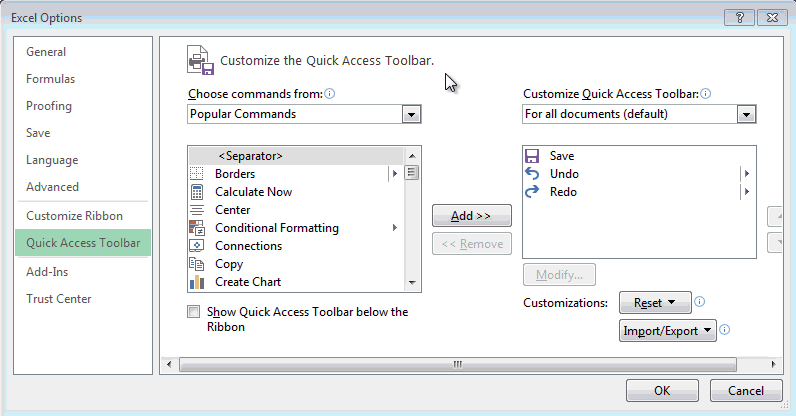
Now, the Advanced Document Properties icon appears in the QAT, and I can easily access it with the corresponding Alt+4 shortcut, as shown below.
In addition to adding built-in commands, you can add macros to the QAT. Simply select Macros from the Excel Options dialog, and then pick your macro. Now, you can launch the macro with the corresponding Alt+Number shortcut. I have a macro that sets up my standard worksheet header and I access it with the QAT keyboard shortcut several times a day. This saves quite a bit of time which makes me happy!
If you have other observations about the QAT or related tips or tricks you’d like to share, please post a comment below!
Источник
Customize keyboard shortcuts
You can customize keyboard shortcuts (or shortcut keys) by assigning them to a command, macro, font, style, or frequently used symbol. You can also remove keyboard shortcuts. You can assign or remove keyboard shortcuts by using a mouse or just the keyboard.
Use a mouse to assign or remove a keyboard shortcut
Go to File > Options > Customize Ribbon.
At the bottom of the Customize the Ribbon and keyboard shortcuts pane, select Customize.
In the Save changes in box, select the current document name or template that you want to save the keyboard shortcut changes in.
In the Categories box, select the category that contains the command or other item that you want to assign a keyboard shortcut to or remove a keyboard shortcut from.
In the Commands box, select the name of the command or other item that you want to assign a keyboard shortcut to or remove a keyboard shortcut from.
Any keyboard shortcuts that are currently assigned to that command or other item appear in the Current keys box, or below the box with the label Currently assigned to.
To assign a keyboard shortcut do the following:
Begin keyboard shortcuts with CTRL or a function key.
In the Press new shortcut key box, press the combination of keys that you want to assign. For example, press CTRL plus the key that you want to use.
Look at Current keys (or Currently assigned to) to see whether the combination of keys is already assigned to a command or other item. If the combination is already assigned, type a different combination.
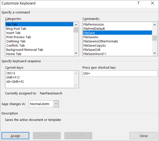
Important: Reassigning a combination of keys means that you can no longer use the combination for its original purpose. For example, pressing CTRL+B changes selected text to bold. If you reassign CTRL+B to a new command or other item, you will not be able to make text bold by pressing CTRL+B unless you restore the keyboard shortcut assignments to their original settings by selecting Reset All at the bottom of the Customize Keyboard dialog box.
Note: If you use a programmable keyboard, the key combination CTRL+ALT+F8 might already be reserved for initiating keyboard programming.
Remove a keyboard shortcut
In the Current keys box, select the keyboard shortcut that you want to remove.
Use just the keyboard to assign or remove a keyboard shortcut
Press ALT+F, T to open the Word Options dialog box.
Press DOWN ARROW to select Customize Ribbon.
Press the TAB key repeatedly until Customize is selected at the bottom of the dialog box, and then press ENTER.
In the Categories box, press DOWN ARROW or UP ARROW to select the category that contains the command or other item that you want to assign a keyboard shortcut to or remove a keyboard shortcut from.
Press the TAB key to move to the Commands box.
Press DOWN ARROW or UP ARROW to select the name of the command or other item that you want to assign a keyboard shortcut to or remove a keyboard shortcut from.
Any keyboard shortcuts that are currently assigned to that command or item appear in the Current keys box, or below the box with the label Currently assigned to.
To assign a keyboard shortcut do the following:
Begin keyboard shortcuts with CTRL or a function key.
Press the TAB key repeatedly until the cursor is in the Press new shortcut key box.
Press the combination of keys that you want to assign. For example, press CTRL plus the key that you want to use.
Look at Current keys (or Currently assigned to) to see whether the combination of keys is already assigned to a command or other item. If the combination is already assigned, type a different combination.
Important: Reassigning a combination of keys means that you can no longer use the combination for its original purpose. For example, pressing CTRL+B changes selected text to bold. If you reassign CTRL+B to a new command or other item, you will not be able to make text bold by pressing CTRL+B unless you restore the keyboard shortcut assignments to their original settings by selecting Reset All at the bottom of the Customize Keyboard dialog box.
Press the TAB key repeatedly until the Save changes in box is selected.
Press DOWN ARROW or UP ARROW to highlight the current document name or template in which you want to save the keyboard shortcut changes, and then press ENTER.
Press the TAB key repeatedly until Assign is selected, and then press ENTER.
Note: If you use a programmable keyboard, the key combination CTRL+ALT+F8 might already be reserved for initiating keyboard programming.
To remove a keyboard shortcut
Press the TAB key repeatedly until the Save changes in box is selected.
Press DOWN ARROW or UP ARROW to highlight the current document name or template in which you want to save the keyboard shortcut changes, and then press ENTER.
Press the SHIFT+TAB key repeatedly until the cursor is in the Current keys box.
Press DOWN ARROW or UP ARROW to select the keyboard shortcut that you want to remove.
Press the TAB key repeatedly until Remove is selected, and then press ENTER.
Источник
Keyboard Shortcuts in Excel


What are Excel Shortcuts?
An Excel shortcut is a technique of performing a manual task in a quicker way. The shortcuts help speed up the work, which saves time for the secondary tasks of the job. Since Excel is used by almost everybody in some form or the other, it is essential to be aware of the shortcuts.
For example, the excel shortcut “Ctrl+O” opens an already existing workbook. The shortcut “Ctrl+W” closes the currently active workbook.
The purpose of using an excel shortcut is to save the worksheet creator from extra clicks. This improves the productivity at the workplace.
At times, the same task is repeated in Excel on a daily basis. Since such tasks may not have a shortcut, the solution is to create it by recording a macro.
Table of contents
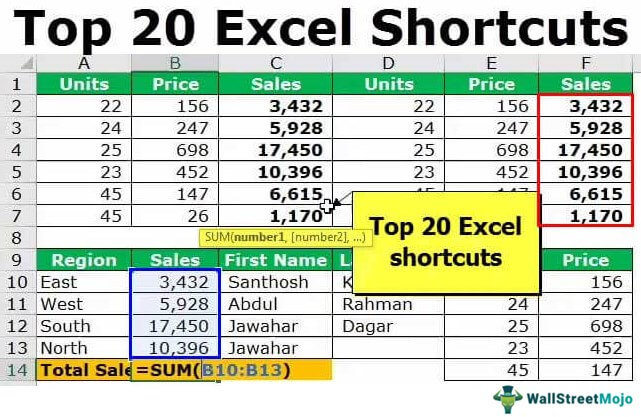
Top 20 Keyboard Shortcuts in Excel
This article discusses the important excel shortcuts which have been consolidated keeping in mind the day-to-day needs of the user. The explanation of each technique is followed by a relevant example.
It is not possible to memorize every excel shortcut. However, a regular usage does allow gradual learning. To develop expertise in Excel, it is imperative to go beyond the basic cut (Ctrl+X), copy (Ctrl+C), and paste (Ctrl+V) shortcuts.
#1–Paste as Values With “Paste Special”
The excel shortcut “Alt+E+S+V” (press one by one) opens the “paste special” window and selects “values” under “paste.”
Note: Prior to pressing the excel shortcut, the formula cell must be copied and the desired output cell (where output is required) should be selected.

Example
The succeeding table shows the prices (in $ in column B) at which some units (column A) of a product are sold. We want to calculate the sales figures and, instead of formulas, paste the final values in column C.
Use the shortcut of the “paste special” property.
The steps to calculate sales and apply the “paste special” shortcut are listed as follows:
Step 1: In cell C2, enter the following formula.
The cell C2 is dependent on the cells A2 and B2.
Copy-paste or drag the formula to the remaining cells. The formulas are applied to the entire range (C2:C6).

Step 2: Copy the formula cell C2. Press the keys “ALT+E+S+V” one by one. The “paste special” window opens. “Values” is automatically selected under “paste.” Click “Ok.”

Step 3: The number 3,432 is pasted in cell C2 as a value and not as a formula.

#2–Sum Numbers With AutoSum
The shortcut “Alt+=” (press together) sums numbers.

Example #2
The following table shows the region-wise sales of an organization. We want to sum all the sales figures to find the total sales. Use the shortcut of AutoSum.
Step 1: Select cell B6. Press the excel shortcut keys “Alt+=” together.
Step 2: The SUM formula automatically appears in cell B6, as shown in the following image.
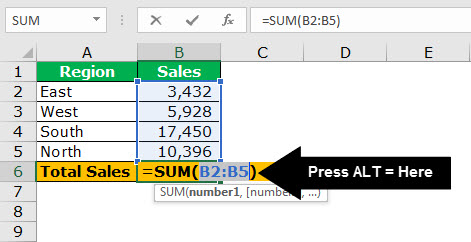
#3–Fill the Subsequent Cell With the Fill Down
The fill down Fill Down When you want to fill down or copy any data or formulas to the cells down below, you can use Excel fill down. While copying the data and selecting the cells, the keyboard shortcut is CTRL + D. read more property fills the present (subsequent) cell with the value or formula of the immediately preceding cell. This feature is often used while entering data in Excel.
The excel shortcut “Ctrl+D” (press together) fills the immediately following cell with the data or formula of the preceding cell.
If a range of cells is selected, the content of the topmost cell is filled in the cells below. If the subsequent cell already contains a value, pressing “Ctrl+D” overwrites it.
Note 1: If the preceding cell contains a value, the fill down feature copies the same to the immediately following cell. However, if the preceding cell contains a formula, the same is copied.
Note 2: While copying a formula, the cell references may or may not change depending on the kind of references used (relative or absolute).
Note 3: The shortcut “Ctrl+D” works only for columns and not for rows. For rows, use the shortcut “Ctrl+R” (press together), which fills cells to the right.

Example
The left side of the following image shows the first and the last names in columns A and B respectively. We want to copy the first name of row 4 in row 5 with the help of the fill down excel shortcut.
Step 1: Select cell A5. Press the keys “Ctrl+D” together.
Step 2: The name “Jawahar” is copied to cell A5, as shown by the right side of the following image.

Example
The left side of the following image shows the sales (column G) calculated by multiplying the price (column F) with the number of units (column E).
We want to calculate the sales (units=45 and price=26) for the entry in row 7. Use the fill down shortcut.
Step 1: Enter 26 as the price in cell F7. Select cell G7 and press the keys “Ctrl+D.”
Step 2: The formula of the preceding cell (G6) is copied to cell G7, as shown by the right side of the following image.

#4–Select the Entire Row or Column
Often, there is a need to select the entire row or column in Excel.
The excel shortcut “Shift+space” (press together) selects the entire row.

The shortcut “Ctrl+space” (press together) selects the entire column.

Example
The following image shows a blank worksheet. With the help of the shortcut, we want to:
a) Select row 4 in the given worksheet
b) Select column B in the given worksheet
a) Step 1: Select any cell in row 4. Press the excel shortcut keys “Shift+space” together.
Step 2: The entire row 4 is selected, as shown in the following image.

b) Step 1: Select any cell in column B. Press the shortcut keys “Ctrl+space” together.
Step 2: The entire column B is selected, as shown in the following image.

#5–Insert and Delete Row or Column
The excel shortcut “Ctrl+Shift+plus sign (+)” inserts a new row or column. The keys must be pressed together.
Prior to pressing this shortcut, select the entire row or column preceding which the insertion has to be made. For this, click the row or column label appearing at the leftmost side or on top.

The excel shortcut “Ctrl+minus sign (-)” deletes an existing row or column. The keys must be pressed together.
Prior to pressing this shortcut, select the entire row or column which has to be deleted.

Note: If the preceding shortcuts (insert or delete) are pressed by selecting a cell rather than the entire row or column, the “insert” or “delete” dialog box opens.
Example
The following image shows the number of units (column E), prices (column F), and sales (column G). With the help of the shortcut, we want to:
a) Insert a row preceding row 4
b) Delete the newly inserted row 4.
a) Step 1: Select the entire row 4 by clicking the label “4” at the leftmost side.
Step 2: Press the keys “Ctrl+Shift+plus sign (+)” together.
Step 3: A row preceding row 4 is inserted, as shown in the following image.

b) Step 1: Click the row label to select the entire row 4.
Step 2: Press the keys “Ctrl+minus sign(-)” together.
Step 3: The newly inserted row (inserted in step 3 of the preceding solution) is deleted. The same is shown in the following image.

#6–Insert and Edit Comment
In Excel, we may need to enter comments for a specific cell. This saves the information related to that cell and allows returning to the same, if required.
The excel shortcut “right-click+M” (press one by one) inserts a new comment on a cell.
The right-click button (menu or the context key) on the keyboard opens the context menu for the selected item. The menu key is located at the bottom, to the right side of the spacebar. It is placed between the right side “Alt” and the right side “Ctrl” key.
Prior to pressing the shortcut, it is important to select the cell in which a comment is to be inserted.
Note: Alternatively, press “Shift+F10” (press together) to open the context menu. Thereafter, press “M” to insert a comment.

The excel shortcut “Shift+F2” (press together) helps edit a comment.
Prior to pressing the shortcut, select the cell containing the comment to be edited.

Example
Working on the data of example #6, we want to:
a) Insert a comment on cell C2
b) Edit the comment of cell C2
Use the shortcut of inserting and editing comments.
a) Step 1: Select the cell C2. Press the menu key followed by “M.”
Step 2: A comment is inserted on cell C2, as shown in the following image.

b) Step 1: Select the cell C2. Press the keys “Shift+F2” together.
Step 2: The cursor appears inside the comment. The comment can now be edited, as shown in the following image.

#7–Move Between Sheets
While working in Excel, different sheets are required to be dealt with at one time. Moreover, it is tedious to click the sheet labels at the bottom of the workbook. The shortcuts help in quickly navigating through the sheets.
The excel shortcut “Ctrl+page down” (press together) helps move from the currently active sheet to the next sheet.

The excel shortcut “Ctrl+page up” (press together) helps move from the currently active sheet to the preceding sheet.

For example, the sheet names are “sheet 1,” “sheet 2,” and “sheet 3” and the current active sheet is “sheet 2.” To go to “sheet 3,” press “Ctrl+page down.” Press “Ctrl+page up” to move to “sheet 1.”
Example
The following image shows the different data sheets of a workbook. With the help of the excel shortcut, we want to:
a) Move from the “insert comment” sheet to the “freeze rows & column” sheet
b) Move from the “freeze rows & column” sheet back to the “insert comment” sheet
a) Step 1: Press the keys “Ctrl+page down” together.
Step 2: There is a movement from “insert comment” to “freeze rows & column” sheet. The latter sheet is now the currently active sheet.

b) Step 1: Press the keys “Ctrl+page up” together.
Step 2: There is a movement from “freeze rows & column” to “insert comment” sheet. The currently active sheet now is the “insert comment” sheet.

#8–Add Filters
The excel shortcuts “Ctrl+Shift+L” (press together) or “Alt+D+F+F” (press one by one) add and remove filters.


Example
Working on the data of example #6, we want to insert filters on columns A, B, and C. Thereafter, remove these filters. Use the shortcut keys.
Step 1: Select cell A1. Press the keys “Ctrl+Shift+L” together. Alternatively, press the keys “Alt+D+F+F” one by one.
Step 2: The filters are added to columns A, B, and C.
Step 3: Press the preceding shortcuts (pressed in step 1) again. The filters are removed.
The insertion and removal of filters are shown in the following image.

#9–Freeze Rows and Columns
While working in Excel, there may be a need to freeze the first row and the first column. Once frozen, the given row and column do not move while scrolling through the remaining data.
The excel shortcut “Alt+W+F+F” (press one by one) freezes the rows and/or columns based on the current selection of cell.
To freeze the first row and the first column, select cell B2.
Note: The given shortcut freezes the rows preceding the currently selected cell. At the same time, the columns to the left of the currently selected cell are also frozen.

Example
The following image shows the username and the passwords in columns A and B respectively. We want to freeze the first row and the first column with the help of the shortcut keys.
Step 1: Select cell B2. Press the shortcut “Alt+W+F+F” one by one.
Step 2: The first row and the first column are frozen, as shown in the following image.

#10–Open “Format Cells” Dialog Box
The “format cells” dialog box helps format a cell or a cell range of Excel. To open this box manually, select a cell and right-click the same. Thereafter, choose the “format cells” option from the context menu.
The shortcut “Ctrl+1” (press together) opens the “format cells” dialog box.

Example
We want to open the “format cells” dialog box in an Excel worksheet with the help of the shortcut.
Step 1: In the worksheet, press “Ctrl+1” together.
Step 2: The “format cells” dialog box appears, as shown in the following image.

#11–Adjust Column Width
The excel shortcut “Alt+O+C+A” (press one by one) adjusts the width of the selected column.

Example
The left side of the following image shows the usernames in column A. Since the width of this column has not been adjusted, some entries are exceeding its right-side border.
We want to adjust the width of column A with the help of the shortcut keys.
Step 1: Select the column (column A) whose width has to be adjusted.
Step 2: Press the shortcut keys “Alt+O+C+A” one by one.
Step 3: The column width is adjusted, as shown by the right side of the following image. Hence, all entries fit in column A.
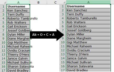
#12–Repeat the Last Task
In Excel, one may need to repeat the last task or action performed. This task can be formatting, inserting a new row or column, deleting an existing row or column, and so on.
The shortcut “F4” repeats the last task, if possible.

#13–Insert Line Breaks in a Cell
While typing in a cell, there may be a need to insert a line break. The line break helps add spacing between the sentences of a cell. Once a line break is added, the user can begin a new sentence in the same cell.
The excel shortcut “Alt+Enter” (press together) inserts a line break within a cell.

Example
The following image shows a question in cell A1. We want to insert a line break in order to type a new sentence within the same cell A1. Use the shortcut for the same.
Step 1: Double-click the cell (cell A1) within which a line break is to be inserted.
Step 2: Click at the place (after the two question marks) where the line break is to be inserted.
Step 3: Press the keys “Alt+Enter” together. The line break appears, as shown in the following image. Hence, after the spacing has been inserted, the user can begin a new sentence in cell A1.

#14–Move Between Different Workbooks
To switch between various windows, the shortcut “Alt+tab” is used. However, often while working, one needs to move from one workbook to another.
The excel shortcut “Ctrl+tab” (press together) helps switch between the open workbooks.

#15–Spell-Check
Prior to submitting an Excel worksheet to seniors at the workplace, it is essential to do a quick spell-check. This lets the user know the mistakes and the corrections that should be followed presently and in the future.
The excel shortcut “F7” helps perform a spell-check of the currently active worksheet.

Example
The following image shows the usernames in column A. We want to run a spell-check on this worksheet with the help of the shortcut.
Step 1: Press the shortcut “F7.”
Step 2: The “spelling” dialog box appears, as shown in the following image. Hence, the spellings of column A can be corrected by matching them against the suggestions.

#16–Move Between Worksheet and Excel VBA Editor
The excel shortcut “Alt+F11” helps switch between the VBA editor and the worksheet.
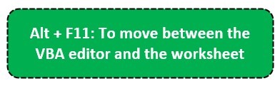
#17–Select a Cell Range
Selecting the cell ranges of Excel can be a time-consuming task, if done manually.
The excel shortcut “Ctrl+Shift+arrow keys” selects the cell ranges of Excel.
Note: The selection of cells, in the same row or column as the currently active cell, is carried out till the last non-blank cell. However, if the following cell (in the same row or column as the currently active cell) is blank, the selection is carried out till the next non-blank cell.

Example
The following image shows the usernames, passwords, designations, titles, and first names in columns A, B, C, D, and E respectively. We want to select the range A1:E100 with the help of the shortcut.
Step 1: Select cell A1. Press the keys “Ctrl+Shift+right arrow” to select till cell E1.
Step 2: Press the keys “Ctrl+Shift+down arrow” to select till cell E100.
Step 3: The range A1:E100 is selected, as shown in the following image.
![]()
#18–Select the Last Non-Blank Cell of a Row or Column
Beginning from cell A1, one may need to go to the last cell of column A. This requires manual scrolling, which is a difficult task, particularly when working with large datasets.
The excel shortcut “Ctrl+down arrow” (press together) helps the user go to the last non-blank cell of the current column (column of the active cell).

The excel shortcut “Ctrl+right arrow” (press together) helps the user go to the last non-blank cell of the current row (row of the active cell).

Note: In case the cell immediately following the active cell is blank, the next non-blank cell is selected.
Example
The following table shows the usernames and passwords in columns A and B respectively. We want to go to the cell A100, which is the last non-blank cell of column A. Use the shortcut keys.
Step 1: Select cell A1. Press the keys “Ctrl+down arrow” together.
Step 2: The last cell (A100) of the dataset is selected, as shown in the following image.
![]()
#19–Delete the Active Sheet
To delete a sheet manually, one can right-click the sheet name and select “delete.” Alternatively, the shortcut helps do the same quickly.
The excel shortcut “Alt+E+L” (press one by one) deletes the currently active sheet.
Once the given shortcut is pressed, a message appears stating that the data of the worksheet will be permanently deleted. Click “delete” to delete the sheet, otherwise press “cancel.”

#20–Insert a New Sheet
Often, new sheets are required to be added to the workbook. It is possible to insert a new sheet with a single click.
The excel shortcut “Shift+F11” (press together) inserts a new sheet in the current workbook.

The excel shortcut “F11” inserts a chart sheet in which a chart can be created by selecting a data range.

Frequently Asked Questions
An Excel shortcut helps perform a manual task in a faster way. With the application of shortcuts, the user saves time and improves the productivity. This saved time can be used for focusing on other projects of a job role.
The list of Excel shortcuts is a large one. There are shortcuts for entering, formatting, deleting, and selecting data. So, it is not possible to learn all the shortcuts. However, knowing the regularly used ones is essential.
To use an Excel shortcut, press the particular keys on the keyboard. But, prior to using it, one must know whether to press the keys simultaneously or one by one. This is because each shortcut works in a specific way.
The basic Excel shortcuts are listed as follows:
Ctrl+S: It saves a workbook.
Ctrl+A: It selects the entire worksheet.
Ctrl+B: It makes the content of the selected cells bold.
Ctrl+C: It copies the selected cell.
Ctrl+I: It italicizes the content of the selected cell.
Ctrl+P: It opens the “print” dialog box.
Ctrl+X: It cuts the content of the selected cell.
Ctrl+V: It pastes in the currently selected cell.
Ctrl+Z: It undoes the last action.
Excel shortcuts can be learned with regular usage and practice. The more you practice working on Excel, the more habitual you will become. In this way, you can learn gradually.
Note: The keys of all the preceding shortcuts should be pressed simultaneously.
The “tab” key is an important shortcut used for auto-completing the name of the function. For instance, to enter the CONCATENATE function in a cell, type “=CON” and press the “tab” key. The CONCATENATE function is automatically selected.
With the “F4” key, one can toggle between the relative, absolute, and mixed references. Double-click the formula cell and press “F4” to change the type of reference.
Likewise, different keyboard keys have different functions. By applying shortcuts to Excel formulas, one can simplify working with calculations.
Recommended Articles
This has been a guide to the top 20 keyboard shortcuts in Excel. Here we discuss the working of keyboard shortcuts and how to use these Excel shortcuts to save your time. You may learn more about Excel from the following articles-
 Adnan Ahmed says
Thank you very much for your efforts
Dheeraj Vaidya says
Thanks for your kind words!
Kufreh says
Very helpful, I am glad you share.
Thank you
Lalit Kumar says
Источник
Generally, you can improve your speed by keeping your hands on your keyboard. But, what do you do if there is no built-in keyboard shortcut to execute your favorite command? Well, one approach is to customize the QAT. This post discusses the Quick Access Toolbar and the related keyboard shortcuts it creates.
QAT Shortcuts
Microsoft introduced the Quick Access Toolbar (QAT) in Excel 2007 with the rollout of the ribbon. It is a tiny little toolbar that includes a few commands by default, such as save, undo, and redo.
You can see it in the following screenshot just above the ribbon:
The nice thing about the QAT is that Excel automatically creates a simple keyboard shortcut to access its command icons. If you tap the Alt key, you’ll notice that the QAT icons each get a sequential number, 1, 2, 3, and so on, as shown below.
The QAT commands are easily accessed by tapping the corresponding Alt+Number combination. This is quite handy, especially since we can customize the QAT to include additional commands.
QAT Customization
Microsoft allows us to customize the QAT, including positioning it above or below the ribbon and adding/removing commands. On the right side of the QAT you’ll see a little dropdown arrow, and when you click it, you’ll have access to the various customization options, as shown below.
Some of the basic commands are provided in the dropdown menu, and you can toggle them on or off. In addition, you can select More Commands to open up the Excel Options dialog to select from a huge number of Excel commands. Remember how the QAT automatically creates an Alt shortcut for its icons? Well, when you add a command to the QAT you’ll be able to access it with a simple Alt shortcut. So, any frequently used commands become a simple shortcut away.
Let’s walk through an example. Back in Excel 2003 and earlier, I could quickly access the document properties dialog box by hitting Alt+F, I. I loved this dialog because it showed the full path of the file and I was able to quickly confirm that I was working on the correct document. I lost that dialog beginning with Excel 2007 and the new document properties didn’t seem to show the full file path. The good news is that it is easy to customize the QAT to regain that dialog. We’ll use this customization as an example, but keep in mind, there are hundreds of commands available to add, so, you can easily customize the QAT to include just your favorites and frequently used commands.
We click the little QAT dropdown and select More Commands to open the Excel Options dialog. Then, we select All Commands from the Choose commands from dropdown, select Advanced Document Properties from the command list, and click the Add button, as shown below.
Now, the Advanced Document Properties icon appears in the QAT, and I can easily access it with the corresponding Alt+4 shortcut, as shown below.
In addition to adding built-in commands, you can add macros to the QAT. Simply select Macros from the Excel Options dialog, and then pick your macro. Now, you can launch the macro with the corresponding Alt+Number shortcut. I have a macro that sets up my standard worksheet header and I access it with the QAT keyboard shortcut several times a day. This saves quite a bit of time which makes me happy!
If you have other observations about the QAT or related tips or tricks you’d like to share, please post a comment below!
Additional Comments
- Beginning with Excel 2010, we can also customize the ribbon by adding new tabs and icons. Investigate it here: Excel Options > Customize Ribbon.
- In addition to adding ribbon icons to the QAT, you can add commands that don’t appear in the ribbon. There are many Excel commands that do not appear in the ribbon, and customizing the QAT is a great way to gain access to them.
Full proficiency in Microsoft Office demands the use of keyboard shortcuts. Although there are plenty of built-in keyboard shortcuts for Microsoft Excel, for the best workflow you usually need to edit or customize those shortcuts to better fit your needs.
Luckily, Excel supports some customizable keyboard shortcuts, and we’re here to show you how to create your own.
A Note on Default Excel Keyboard Shortcuts
Unfortunately, it’s not all perfect in the Excel custom shortcut realm. Excel doesn’t offer the functionality to override standard shortcuts, so you can’t adjust the shortcut key for something that already exists.
Thus, there are three main types of keyboard shortcuts:
- Standard shortcuts, like Ctrl + I for italics, which you cannot change in Excel.
- Alt shortcuts, where you press the Alt key to activate shortcuts for Ribbon items. For example, pressing Alt > N > T will select the Insert tab on the Ribbon, followed by the Table option.
- Macro shortcuts, which are completely customized. We’ll discuss these in a bit.
So while you can’t tweak any of the default shortcuts, you can still access quite a bit of functionality on the Ribbon or create macros. Thus, we’ll use those options to make custom shortcuts.
The Quick Access Toolbar (QAT) is a helpful strip of commands that always stays at the top of your screen. By default, it only includes a few options, such as save, undo, and redo, which you might want to remove, since they already have easy keyboard shortcuts. But you can add many more commands to the QAT.
We mentioned that Alt codes let you access anything on the Ribbon. If you press Alt, you should notice some popup shortcut keys that also appear near the QAT, giving you a one-step shortcut to any Excel command you wish.
To set up the Quick Access Toolbar in Excel as you like, click the dropdown arrow to the far right of the current icons. You can check a few common options here, but for a full list, you’ll want to select More commands.
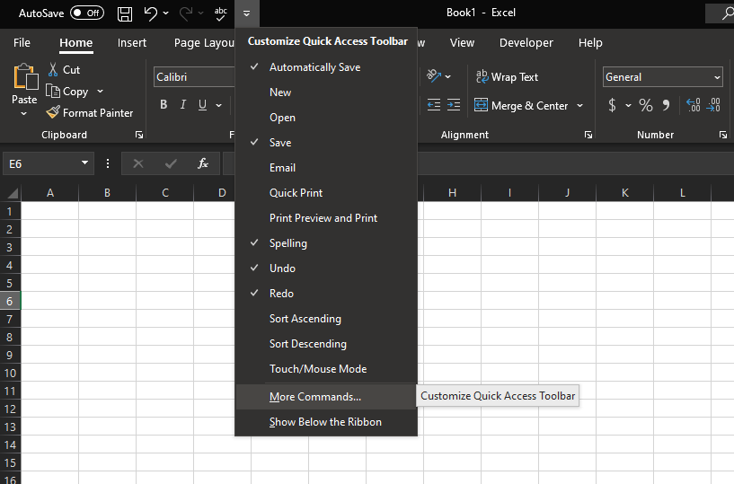
This opens the customization window, where you’ll see a list of available commands in the left box and your current QAT commands on the right.
Customizing the Quick Access Toolbar
Click any command in the right box and hit the Remove button to erase it or use the arrow buttons to the right of the box to re-order the current items. Once you’ve got that sorted, check out the left box to find new commands you want to add.
By default, the dropdown box shows Popular Commands, but you can change it to Commands Not in the Ribbon if you want to avoid duplicating what’s already there. You can also show All Commands, but be warned that there’s quite a long list.
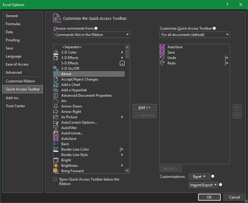
Have a look through the list and select any functions you’d like instant access to. The QAT allows for lots of commands, so don’t be afraid to pick several of your favorites or even find some new features to try.
If you want to create groupings, there’s an option called <Separator> that lets you add a divider between icons. And to preserve your setup for the future, use the Import/Export button in this window to export your customizations.
Once you’ve got everything in order, just click OK to return to Excel with your new and improved QAT. When you want to access one of its functions, press Alt, followed by the number of the command, to execute it right away.
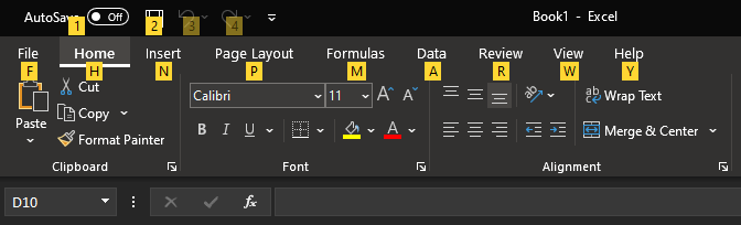
This is a lot faster than hunting through menus to find the right command.
2. Create Your Own Excel Macros
Macros are an extremely useful (yet often overlooked) feature of Office that allow you to record a series of actions and automatically play them back. If you have trouble remembering complex formulas, for example, you could create a macro to automatically apply the formulas to specific cells.
Macros are really just Visual Basic code running in the background to make Excel perform actions, but you don’t have to know how to program to take advantage of macros.
To get started with using them, enable the Developer Ribbon tab by going to File > Options and choose Customize Ribbon on the left pane. On the right side, make sure Developer is checked, then press OK to return.
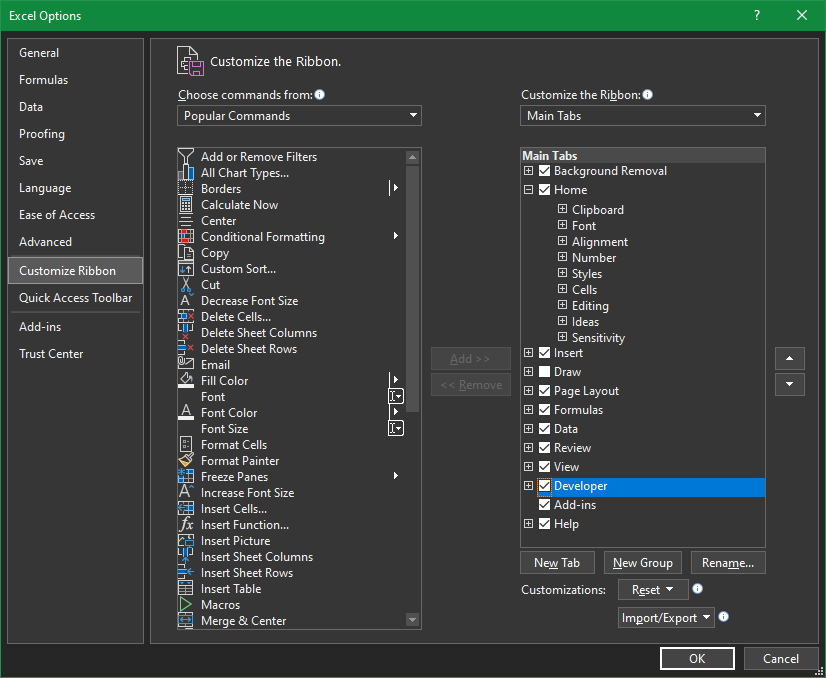
Recording New Macros
Now you can record your first macro. Head to the Developer tab on the Ribbon and choose Record Macro in the Code section. Give it a name to remember it by (it can’t have spaces) and assign it a key that works for you.
The shortcut box shows Ctrl + another key, but you can also add Shift to this by holding it while you select a key. Bear in mind that you can override standard keyboard shortcuts here, so if you make your macro run with Ctrl + Z, you won’t be able to use that shortcut to undo anymore.
Under Store macro in, select Personal Macro Workbook. This is a file that allows you to share macros between Excel workbooks, which is perfect for defining shortcuts. If you want to run macros on only one workbook, change this setting to This Workbook instead. Give your macro a brief description if you like, then click OK.
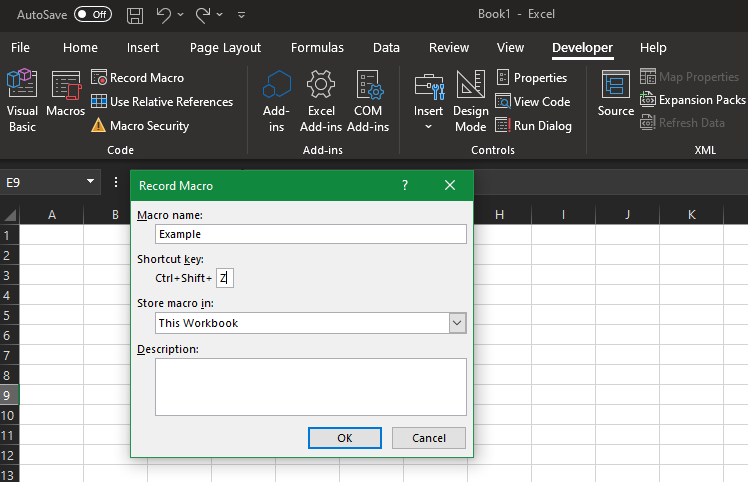
From here, everything you do is recorded. Any cell you select, font changes you apply, or characters you type become your macro. So you could, for example, make a macro that selects cell B3, types «test,» and formats it as bold. Once you’ve performed exactly the action you want to record, select Stop Recording on the Developer tab to end the macro.
Using and Editing Macros
After this, you can access your macro by choosing Macros from the same Code section of the Developer tab. This shows a list of your macros; press Edit to view the Visual Basic code for the macro, if you like. This is a good way to make sure you didn’t record any extra steps, even if you don’t fully understand the code.
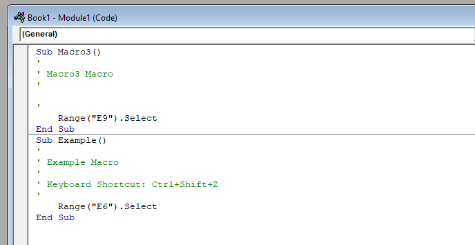
Once you’re satisfied, you can press the key combo you assigned at any time to run your macro. To change the key combination later, select it in the list of Macros and choose Options.
Here’s an advanced tip: you can even combine macros and the QAT. Once you’ve saved a macro, open up the QAT menu again and change the Choose commands from box to Macros. Select a macro you’ve created from the list, and you can add it to the QAT just like any other action.
Thus, if you have trouble remembering macro shortcut combos, you can instead run them from the QAT with Alt and a number.
What you do with macros is up to you, but there are tons of possibilities. Think of anything you do in Excel on a regular basis that you’d want to automate, and try making a macro for it. Automating these tedious tasks can save you hours of time.
Have a look at our guide to making Excel macros for more ideas and help.
Easily Create Custom Excel Shortcuts
Now you don’t have to waste time performing repetitive tasks or hunting through Excel menus to find a particular feature. Shortcuts take a bit to set up and everyone will want different ones, but they’re vital for Excel efficiency.
Macros aren’t scary once you’ve done a few, and the QAT is handy for everyone. But those aren’t the only timesavers Excel is hiding.
Image Credit: GooDween123/Shutterstock
Требуется полная эффективность пакета для повышения производительности. Microsoft Офис Используйте сочетания клавиш. Хотя есть много встроенных сочетаний клавиш для Microsoft Excel Однако для оптимального рабочего процесса вам обычно необходимо отредактировать или настроить эти ярлыки в соответствии с вашими потребностями.
К счастью, Excel поддерживает несколько настраиваемых сочетаний клавиш, и мы здесь, чтобы показать вам, как создать свои собственные.
К сожалению, не все идеально в области настраиваемых ярлыков в Excel. Excel не предоставляет функции для переопределения стандартных сочетаний клавиш, поэтому вы не можете назначить сочетание клавиш для того, что уже существует.
Таким образом, существует три основных типа сочетаний клавиш:
- Стандартные сокращения, например Ctrl + I Для курсива, который нельзя изменить в Excel.
- Ярлыки другой , где вы нажимаете клавишу другой Активирует ярлыки для элементов ленты. Например, нажатие. Будет Alt -> N -> T Для выбора вкладки Вставлять в баре, а затем вариант جادول.
- Ярлыки макросов, которые полностью настраиваются. Об этом мы поговорим ниже.
Таким образом, хотя вы не можете изменить какие-либо ярлыки по умолчанию, вы все равно можете получить доступ к большому количеству функций на ленте или создавать макросы. Таким образом, мы будем использовать эти параметры для создания пользовательских ярлыков.
1. Пользовательские ярлыки панели быстрого доступа
Панель быстрого доступа (QAT) — это полезная панель команд, которая всегда находится в верхней части экрана. По умолчанию он включает только несколько параметров, таких как «Сохранить», «Отменить» и «Повторить», которые вы, возможно, захотите удалить, поскольку в нем уже есть простые сочетания клавиш. Но вы можете добавить больше команд в QAT.
Мы упоминали, что аббревиатура другой Позволяет получить доступ ко всему на ленте. Если вы нажмете другой Затем вы должны заметить несколько всплывающих горячих клавиш, которые также появляются рядом с QAT, что дает вам одношаговый ярлык для любой команды Excel, которую вы хотите.
Чтобы настроить панель быстрого доступа Excel так, как вы хотите, щелкните стрелку раскрывающегося списка справа от текущих значков. Здесь вы можете ознакомиться с некоторыми из популярных опций, но для получения полного списка вам нужно выбрать больше команд.
Откроется окно настройки, в котором вы увидите список доступных команд в левом поле и текущие команды QAT справа.
Настроить панель быстрого доступа
Щелкните любую команду в правом поле и нажмите кнопку «زالةчтобы удалить его, или используйте кнопки со стрелками справа от поля, чтобы переставить текущие элементы. Когда вы закончите, установите флажок в левом поле, чтобы найти новые команды, которые вы хотите добавить.
По умолчанию в раскрывающемся списке отображаются общие команды, но вы можете изменить их на команды, которых нет на ленте, если вы хотите избежать повторения того, что уже есть. Вы также можете просмотреть все команды, но имейте в виду, что список очень длинный.
Взгляните на список и выберите любые функции, к которым вы хотите получить мгновенный доступ. QAT позволяет использовать множество команд, поэтому не бойтесь выбрать несколько избранных или даже попробовать новые функции.
Если вы хотите создавать группы, есть опция под названием Позволяет добавить разделитель между символами. А чтобы сохранить настройки на будущее, используйте кнопку импорта / экспорта в этом окне, чтобы экспортировать свои настройки.
Когда все будет в нужном порядке, просто нажмите «OkЧтобы вернуться в Excel и использовать новый улучшенный QAT. Если вы хотите получить доступ к одной из его функций, нажмите другой , за которым следует номер команды, чтобы выполнить ее немедленно.
Это намного быстрее, чем поиск нужной команды в меню.
2. Создайте макросы Excel.
Макросы — это очень полезная (и часто упускаемая из виду) функция Office, которая позволяет записывать и автоматически воспроизводить серию действий. Если, например, у вас возникли проблемы с запоминанием сложных функций, вы можете создать макрос для автоматического применения функций к определенным ячейкам.
На самом деле макросы — это просто код Visual Basic, работающий в фоновом режиме, чтобы Excel выполнял действия, но вам не нужно знать, как программировать, чтобы воспользоваться преимуществами макросов.
Чтобы начать использовать его, включите вкладку Разработчик, перейдя в Файл -> Параметры И выберите Настроить ленту на левой панели. И под основными вкладками установите флажок Разработчик , затем нажмите Ok Возвращать.
Запись новых макросов
Теперь вы можете записать свой первый макрос. Перейдите на вкладку Разработчик на ленте и выберитеЗапись макросав разделе Код. Дайте ему имя, которое нужно запомнить (оно не может содержать пробелов), и назначьте сочетание клавиш, которое подойдет вам.
В поле сочетания клавиш отображается Ctrl + другая клавиша, но вы также можете добавить к нему Shift, нажав его, когда клавиша выбрана. Имейте в виду, что здесь вы можете переопределить стандартные сочетания клавиш, поэтому, если вы запустите макрос с Ctrl + Z Вы больше не сможете использовать этот ярлык для отмены.
в Сохраните макрос в , Найдите Личная книга макросов. Excel создает скрытую личную книгу макросов (личный .xlsb), если ее еще нет, и сохраняет макрос в этой книге, что идеально подходит для определения ярлыков. Если вы хотите, чтобы макросы выполнялись только в одной книге, измените этот параметр на Эта книга. Введите краткое описание макроса, если хотите, затем коснитесь Ok.
Отсюда все, что вы делаете, регистрируется. Любая выбранная вами ячейка, применяемые вами изменения шрифта или вводимые символы становятся вашими макросами. Так, например, вы можете создать макрос, который выбирает ячейку B3, набирает «тест» и форматирует ее полужирным шрифтом. После того, как вы выполнили именно то действие, которое хотите записать, выберите Остановить запись На вкладке «Разработчик» завершите макрос.
Используйте и редактируйте макросы
После этого вы можете получить доступ к макросам, Выбор макросов Из того же раздела кода на вкладке Разработчик. Это отображает список ваших макросов; Если хотите, нажмите Edit, чтобы просмотреть код Visual Basic для макроса. Это хороший способ убедиться, что вы не записываете никаких дополнительных шагов, даже если вы не совсем понимаете программирование.
Когда вы будете удовлетворены, вы можете нажать назначенную комбинацию горячих клавиш в любое время, чтобы запустить макрос. Чтобы позже изменить комбинацию клавиш, выберите ее в списке макросов и выберите опции.
Вот расширенный совет: Вы даже можете комбинировать макросы и QAT. После сохранения макроса снова откройте меню QAT и измените флажок «Команды» на «Макросы». Выберите созданный вами макрос из списка, и вы можете добавить его в QAT, как и любое другое действие.
Таким образом, если у вас возникли проблемы с запоминанием наборов ярлыков макросов, вы можете вместо этого запускать их из QAT с помощью ярлыка другой и номер.
Что делать с макросами — решать вам, но есть много возможностей. Подумайте обо всем, что вы регулярно делаете в Excel, что вы хотите автоматизировать, и попробуйте создать для этого макрос. Автоматизация этих утомительных задач может сэкономить вам часы времени.
Легко создавайте собственные ярлыки Excel
Теперь тебе не нужно тратить время на Выполняйте повторяющиеся задачи Или выполните поиск в списках Excel, чтобы найти конкретную функцию. Для настройки требуется немного времени, и всем нужны разные сочетания клавиш, но они необходимы для эффективности Excel.
Макросы не пугают после того, как вы их использовали, а QAT подходит для всех. Но он скрывает не только экономию времени. Excel.
Create Custom Excel Shortcuts (2 Ways)
by Avantix Learning Team | Updated March 24, 2021
Applies to: Microsoft® Excel® 2013, 2016, 2019 and 365 (Windows)
Microsoft Excel has many built-in shortcuts as well as the ability to navigate and select in the Ribbon using the keyboard. However, you may also want to write your own keyboard shortcuts for specific commands.
Unfortunately, Excel doesn’t offer a keyboard assignments command similar to the one available in Microsoft Word. In Word, you can assign keyboard shortcuts through the Options command on the File tab. In the Customize Ribbon category, there is a Keyboard Shortcuts Customize button that is not available in Excel.
Recommended article: 10 Excel Data Entry Tricks and Shortcuts Every User Should Know
Do you want to learn more about Excel? Check out our virtual classroom or live classroom Excel courses >
So, you have a couple of options in Excel. You can add buttons to the Quick Access toolbar (which are automatically assigned Alt shortcuts) or you can write a macro using the Macro Recorder.
1. Creating a keyboard shortcut by customizing the Quick Access Toolbar
To customize the Quick Access Toolbar and create keyboard shortcuts:
- Click the File tab in the Ribbon and then click on Options.
- Click the Quick Access Toolbar category on the left.
- From the drop-down menu under Choose commands from, select All Commands.
- Click the button you want to add.
- Click Add.
- Continue adding buttons.
- If you want to re-order buttons, click the button in the Customize Quick Access toolbar pane on the right and click the Move Up or Move Down arrow buttons.
- Click Close.
Commands appear in the Excel Options dialog box:

Once you have added the desired buttons, Excel assigns keyboard shortcuts automatically to the buttons based on the order in the Quick Access Toolbar. For example, the first button can be accessed by pressing Alt and then 1, the second button by pressing Alt and then 2 and so on.
2. Creating a macro with a keyboard shortcut using the Macro Recorder
You can also add a keyboard shortcut by recording a macro. In Excel, you can record a macro to automate specific actions and you can assign a keyboard shortcut to the macro. To keep things simple, we’ll use the Record Macro button on the View tab in the Ribbon.
You’ll be using the Record Macro dialog (below) to create keyboard shortcuts:

To create a macro and assign a keyboard shortcut:
- Open the file you want to use or create a new workbook.
- Click the View tab in the Ribbon.
- Click Macros and select Record Macro. A dialog box appears.
- Under Macro Name, name the macro (no more than 255 characters and do not include spaces or begin with a number or an underscore).
- Under Shortcut key, enter a keyboard shortcut. For example, type Shift + H (this would assign Control + Shift + H as the shortcut). By adding Shift, you are less likely to create the same shortcut as a built-in Excel shortcut.
- Under Store macro in, choose This Workbook, New Workbook or Personal Macro Workbook. For global shortcuts, save the macro in the Personal Macro Workbook which is launched on startup and is hidden by default. If you store a macro in another workbook, it will need to be open to run the macro.
- Under Description, you can enter a description.
- Click OK.
- Perform the actions you want to record. For example, click Paste on the Home tab, choose Paste Special and then click on Values in the dialog box. All of your actions are being recorded.
- Click the View tab, click on Macros and then select Stop Recording.
- Try pressing the keyboard shortcut combination that you assigned to run the macro.
When you use the Macro Recorder, Excel writes the code for the macro using VBA (Visual Basic for Applications). If a macro you created in the Personal Macro Workbook doesn’t work as expected, you will probably want to delete it.
To delete a macro that is stored in the Personal Macro Workbook, you will need to unhide the workbook first. To unhide the Personal Macro Workbook, click Unhide on the View tab, click Personal and click OK. To delete a macro, click Macros on the View tab and choose View Macros. Click on the macro you want to delete and click Delete. Be sure to hide the Personal Macro Workbook again using Hide on the View tab.
If you have displayed the Developer tab in the Ribbon, Record Macro as well as other useful buttons appear in this tab as well.
Subscribe to get more articles like this one
Did you find this article helpful? If you would like to receive new articles, join our email list.
This article was first published on February 13, 2017 and has been updated for clarity and content.
More resources
How to Fill Blank Cells in Excel with a Value from a Cell Above
How to Use Flash Fill in Excel to Clean or Extract Data (Beginner’s Guide)
How to Quickly Delete Blank Rows in Excel
Related courses
Microsoft Excel: Intermediate / Advanced
Microsoft Excel: Data Analysis with Functions, Dashboards and What-If Analysis Tools
Microsoft Excel: Introduction to Visual Basic for Applications (VBA)
VIEW MORE COURSES >
Our instructor-led courses are delivered in virtual classroom format or at our downtown Toronto location at 18 King Street East, Suite 1400, Toronto, Ontario, Canada (some in-person classroom courses may also be delivered at an alternate downtown Toronto location). Contact us at info@avantixlearning.ca if you’d like to arrange custom instructor-led virtual classroom or onsite training on a date that’s convenient for you.
Copyright 2023 Avantix® Learning
Microsoft, the Microsoft logo, Microsoft Office and related Microsoft applications and logos are registered trademarks of Microsoft Corporation in Canada, US and other countries. All other trademarks are the property of the registered owners.
Avantix Learning |18 King Street East, Suite 1400, Toronto, Ontario, Canada M5C 1C4 | Contact us at info@avantixlearning.ca
Keyboard shortcuts are, perhaps, one of the Excel topics that virtually any user can (or should) be interested in.
This makes sense. The following are some of the reasons that explain this:
- Keyboard shortcuts are extremely useful for purposes of improving your speed and productivity when working with Excel.
Not knowing the right keyboard shortcut means that, instead of quickly typing the relevant key combination, you need to (i) lift your hand from the keyboard, (ii) reach for the mouse in order to do what you want, and (iii) return to the keyboard.
- In the most recent versions of Excel, keyboard shortcuts allow you to work with virtually every command or feature by using the keyboard.
- Regardless of your level of Excel knowledge, you can always learn a new shortcut and, considering the huge amount of Excel keyboard shortcuts that you have available, is likely that you’ll never memorize them all.
 I have already created, and update from time to time, one of the most comprehensive lists of keyboard shortcuts available online. You can find this list of keyboard shortcuts for Excel here. The list is also available for download as a free PDF file called Excel Shortcuts and Hotkeys: The Power Spreadsheets Cheat Sheet. If you want to get the data from the PDF file into Excel, you can use any of these conversion methods (which you can also implement with macros).
There are 3 basic reasons why you should consider learning more than lists when studying keyboard shortcuts:
- Reason #1: Regardless of how comprehensive a keyboard shortcut list is, it’s extremely difficult to map absolutely all of the keyboard shortcuts available in Excel. You may find that, from time to time, even massive keyboard shortcut resources (like my cheat sheet) don’t list the keyboard shortcut for the precise item you need.
Knowing how to find or create a keyboard shortcut by yourself can be quite valuable in these situations.
- Reason #2: Keyboard shortcut lists and cheat sheets only include the built-in default keyboard shortcuts of Excel. This leaves out the options you have for creating custom keyboard shortcuts in Excel by using the Quick Access Toolbar or macros.
- Reason #3: Most of us don’t want or need to learn absolutely all the keyboard shortcuts that exist in Excel. Even if we tried to learn them all, is likely that only a few of us would succeed.
This is where this Excel tutorial comes in. My purpose with this blog post is to provide you with the knowledge you need to master keyboard shortcuts in Excel and become even more productive. Therefore, in addition to explaining the different types of keyboard shortcuts that are available in Excel, I show you some methods you can use to create your own custom keyboard shortcuts. The table of contents below shows the specific topics this blog post covers:
Let’s start with a preliminary introduction about how I suggest you approach keyboard shortcuts in Excel:
How To Approach Keyboard Shortcuts In Excel
Lists and cheat sheets with keyboard shortcuts are great. Most of us want to have them and, as I show below, lots of Excel bloggers and writers (including myself) have created their own version of them.
These amazing lists can, however, be slightly overwhelming if you don’t know how to approach them.
More precisely, if you approach keyboard shortcut cheat sheets with the idea that you’ll quickly learn them all by heart, you’re likely to be disappointed.
This isn’t a bad thing. After all, you probably don’t need to know so many keyboard shortcuts. Furthermore, some of those shortcuts may be for commands or features that you rarely use.
And if it makes you feel better, you’re in good company. You can rest assure that most other Excel users (including very advanced ones), don’t know all the shortcuts either.
Therefore, before you begin to collect lists of keyboard shortcuts or trying to learn every single shortcut you come along, I have 1 basic suggestion:
Don’t overload yourself by trying to learn too many keyboard shortcuts at the same time. You’re unlikely to learn a huge amount of keyboard shortcuts in a very short period of time.
I suggest you start slowly and, perhaps, learn 1 or 2 shortcuts per week. Once you’ve mastered a particular shortcut, learn a new one. As you start gaining more familiarity with Excel keyboard shortcuts, you’ll be able to handle more.
You’ll notice the list of keyboard shortcuts you know and use grows consistently over time.
You may wonder, then, how should you choose which keyboard shortcuts to learn first. My suggestion is that you take the following 2-step approach to determine what keyboard shortcuts to master:
- Step #1: Identify commands or tasks that you constantly execute while working with Excel.
Due to the broad variety of activities people carry out with Excel, this varies from person to person. Your list of most commonly used commands may not look at all like mine. And that’s fine:
Just determine what works for you.
- Step #2: Search and find a keyboard shortcut that allows you to execute that particular command or task.
Once you’ve determined the command or task you want to execute with your keyboard, you’ll have 2 basic options for purposes of searching for the corresponding keyboard shortcut:
- Option #1: Check out a list of keyboard shortcuts prepared by somebody else. I share several of such lists below.
- Option #2: Find a built-in keyboard shortcut or, if there’s no suitable option, create your own keyboard shortcuts.
This option #2 is the topic of this blog post.
I have already created (and update from time to time) a very comprehensive shortcut list that helps you with option #1. However, depending on factors such as the type of command or tasks you need to execute and your own personal preferences, the keyboard shortcuts included in such lists may not (for different reasons) work for you.
Fortunately, Excel provides several options for you to carry out a task or execute a command by using only the keyboard. In addition to the huge amount of built-in keyboard shortcuts that Excel has, you can create your own custom keyboard shortcuts (taking into consideration some requirements and limitations that I explain below).
The following section may help you avoid confusion with the, sometimes, irregular terminology used by different authors when talking about keyboard shortcuts. If you aren’t interested in this particular topic, or already have a good grasp of the topic, please feel free to skip to the next section, which talks about regular keyboard shortcuts.
Excel Keyboard Shortcuts, Keyboard Accelerators, Key Tips And Hotkeys: Terminology
When reading about keyboard shortcuts for Excel, you may find that some authors use the terms “keyboard accelerators”, “Hotkeys” or “Key Tips”. You may find some discussions regarding the exact meaning of each term. Without going into more theoretical discussions regarding the technical meaning of each term, let’s take a look at how I use them in this Excel tutorial:
- Keyboard Shortcuts: I generally use the term “keyboard shortcuts” to refer to the combination of keyboard keys that allows you to carry out a particular task that usually requires the use of a mouse. In some contexts, you may see the term “keyboard accelerators” being used to refer to all of such combinations, while the term “keyboard shortcuts” is reserved to the type of keyboard shortcuts that I refer to as regular keyboard shortcuts.
- Key Tips: The term “Key Tips” is used to refer to certain labels or badges that are displayed by Excel as guidance to help you find what is the appropriate sequence for a Ribbon keyboard shortcut or a Quick Access Toolbar keyboard shortcut. The following image shows how Key Tips look like when they’re turned on:

I explain how you can turn on Key Tips, and use them to work with the Ribbon and the Quick Access Toolbar in the sections below.
- Hotkeys: Hotkeys are similar to Key Tips in the sense that they provide some guidance regarding what is the key that you must press in order to choose a particular option. For purposes of this blog post, the 2 main differences between Hotkeys and Key Tips that you must be of aware of are the following:
Difference #1: As shown in the image below, Hotkeys are displayed as an underlined letter. Key Tips, as explained above, are displayed as labels or badges.
Difference #2: Hotkeys are generally displayed within dialog boxes. Key Tips are displayed in the Ribbon and the Quick Access Toolbar.
The following screenshot of the Paste Special dialog box provides an example of how Hotkeys look like. The arrows point to some of the underlined letters within this dialog box.

I explain how you can work with Hotkeys and dialog box keyboard shortcuts below.


The terms listed above are, however, not necessarily used in exactly the same way by other Excel writers or documents. A possible variation of the terminology, for example, involves using the terms “Hotkeys” and “Key Tips” interchangeably.
Sometimes, authors use the term “keyboard accelerator” to refer to the keyboard shortcuts that you use when interacting with the Ribbon, the Quick Access Toolbar or dialog boxes. These are what I refer to here as Ribbon keyboard shortcuts, Quick Access Toolbar keyboard shortcuts and dialog box keyboard shortcuts. Since Key Tips and Hotkeys (as explained above) appear when you use keyboard shortcuts to work with the Ribbon, the Quick Access Toolbar and dialog boxes, you may see the term “keyboard accelerators” instead of Key Tips and Hotkeys.
You don’t have to worry too much about these differences:
Once you’ve read this Excel tutorial, you’ll have enough knowledge to understand other texts that talk about keyboard shortcuts. Therefore, you’ll easily figure out how the relevant author is using each term.
Now that the terminology is clear, let’s start taking a look at the different types of keyboard shortcuts that you can use in Excel. Let’s begin with:
When talking about keyboard shortcuts for Excel, most people refer to Ctrl combination shortcut keys.
As implied by their denomination, Ctrl combination shortcut keys involve pressing the Ctrl key in combination with some other(s) key(s). In most cases, these keyboard shortcuts are of the following form:
Ctrl + Letter
Some of the most well-known and commonly used keyboard shortcuts fall within this group. Some examples are the following:
- “Ctrl + B” to apply or remove bold formatting.
- “Ctrl + C” to copy.
- “Ctrl + V” to paste.
You can, however, find Ctrl combination shortcut keys that combine Ctrl with other keys. The following are some examples:
- Ctrl + Additional Key.
For example, you can use “Ctrl + 1” to display the Format Cells dialog box, “Ctrl + 5” to apply or remove strikethrough formatting or “Ctrl + [” to go to the direct precedents within the active worksheet.
- Ctrl + Shift + Additional Key.
Some examples of such keyboard shortcuts are “Ctrl + Shift + !” (also expressed as “Ctrl + Shift + 1”) to apply number format or “Ctrl + Shift + A” to insert function arguments (when the function name has already been typed and the insertion point is to the right of the function name).
- Ctrl + Alt + Additional Key.
Perhaps my favorite keyboard shortcut following this form is “Ctrl + Alt + V”, which displays the Paste Special dialog box.
There are, however, additional keyboard shortcuts that aren’t Ctrl combination shortcut keys.
I can’t list all the regular keyboard shortcuts that Excel has here. However, for illustrative purposes, the following are some examples of keyboard shortcuts that aren’t Ctrl combination shortcut keys:
- “Shift + Arrow Keys” extends the selection by 1 cell or, within a cell, selects the character to the right or to the left of the insertion point.
- “Shift + F10” is the equivalent of right-mouse button click. In other words, it displays the context menu for the selected item.
- Tab, among other functions, selects a suggestion provided by the autocomplete feature to complete a formula and move one cell to the right or to next unlocked cell.
- “Alt + Page Down” and “Alt + Page Up” take you 1 screen to the right or 1 screen to the left of the current active sheet.
- F7 displays the Spelling dialog box.
- When a row or column is selected, “Right-Mouse Button + E” inserts copied or cut cells.
- Within a dialog box, the Spacebar performs the action that corresponds to the selected button, or selects or clears a checkbox.
As you can see, these are plenty of different regular keyboard shortcut combinations.
All of the keyboard shortcut examples I provide above are (i) for Excel for Windows and (ii) using the English (USA) keyboard layout. If you’re using Excel on a computer that doesn’t meet these 2 requirements, there will (likely) be some differences in some keyboard shortcuts. For example, if you’re using Excel for Mac, some of the Ctrl combination shortcut keys that Excel for Windows has don’t work.
If you’re interested in lists or cheat sheets with the actual keyboard shortcuts, you may be interested in Excel Shortcuts and Hotkeys: The Power Spreadsheets Cheat Sheet. This is my compilation of keyboard shortcuts, which I update from time to time. In addition to the actual blog post, you can gain immediate free access to the PDF file containing that list.
Ribbon Keyboard Shortcuts for Excel: Key Tips
Excel’s Ribbon is the group of tabs and buttons that you see in the upper section of Excel.

If you’ve used Excel before, you probably know that you can use the Ribbon to carry out the most common tasks in Excel.
In fact, my guess is that you use the Ribbon constantly. Also, if you’re like most Excel users, you probably use the mouse to work with the Ribbon (at least most of the time).
However, thanks to Key Tips, you can get to any tab or button within the Ribbon using only the keyboard. As explained by John Walkenbach in the Excel 2016 Bible:
At first glance, you may think that the Ribbon is completely mouse centric (…). But in fact, the Ribbon is very keyboard friendly.
In this section, I explain what you need to know in order to work with the Ribbon using these Ribbon keyboard shortcuts.
When using Ribbon keyboard shortcuts, you don’t need to hold down all the keys at the same time, as you do with regular keyboard shortcuts. In other words, with Ribbon keyboard shortcuts, you can:
- Press the first key and let it go.
- Press the second key and let it go.
- And continue pressing and releasing the relevant keys that compose the keyboard shortcut.
Now that you know this, let’s take a look at the 3 easy steps you can follow to use Ribbon keyboard shortcuts. After explaining these 3 steps, I show you an example of how you can use Ribbon keyboard shortcuts.
Step #1: Turn Key Tips On
To turn on Key Tips, press either of the following keys:
- Alt.
- F10.
Remember that you don’t need to hold down these keys while carrying out the next steps below.
Step #2: Press The Key(s) That Corresponds To The Ribbon Section You Want To Go To
Once you’ve turned Key Tips on, Excel displays the keys that corresponds to each Ribbon tab, the Backstage View (whose Ribbon label is “File”) and Tell Me (whose Ribbon label is “Tell me what you want to do”).
Tell Me was introduced in Excel 2016. Therefore, if you’re using Excel 2013 or earlier, you won’t have access to this feature.
The following image displays an Excel Ribbon with the Key Tips turned on:

The following table summarizes these Key Tips:
| Tab | Key | Full Keyboard Shortcut To Display Tab |
|---|---|---|
| File (Backstage View) |
F | Alt + F or F10 + F |
| Home | H | Alt + H or F10 + H |
| Insert | N | Alt + N or F10 + N |
| Page Layout | P | Alt + P or F10 + P |
| Formulas | M | Alt + M or F10 + M |
| Data | A | Alt + A or F10 + A |
| Review | R | Alt + R or F10 + R |
| View | W | Alt + W or F10 + W |
| Developer | L | Alt + L or F10 + L |
| Tell me what you want to do | Q | Alt + Q or F10 + Q |
The Ribbon of your particular version of Excel likely looks different from that of the image above. For example:
- You may not see some of the tabs that are displayed above.
This may be the case, for example, if you don’t have the Developer tab enabled.
- You may see additional tabs.
This may be the case, for example, if you have selected an object (such as a chart) and, as a consequence, Excel displays a contextual tab.
For example, I took the following screenshot when a chart is selected. Notice the 2 additional tabs (Design and Format) which you can access by pressing “J + C” (Design) and “J + A” (Format).

- You may not see the Tell Me feature.
This is the case if you’re using Excel 2013 or earlier. The screenshot above was taken using Excel 2016.

However, the Key Tips for the Ribbon tabs remain the same. In other words, “Alt + H” always takes you to the Home tab, “Alt + N” always takes you to the Insert tab, and so on.
Regardless of how your Ribbon looks like, Excel always displays the Key Tips corresponding to all the sections (Ribbon tabs, Backstage View and Tell Me) you can access at that particular time. Just remember the rule you must follow once you’ve turned on the Key Tips:
Press the key(s) that corresponds to the section (usually a tab) of the Ribbon you want to activate.
In fact, as I shown in step #3 below, when you’re working with the Ribbon, you just need to continue applying this rule:
Step #3: Continue Pressing The Key(s) That Corresponds To What You Want To Activate
Once you’ve turned the Key Tips on (as explained in step #1 above), Excel continues to display the Key Tips that correspond to the particular situation you’re in. In other words:
At any given time, the Key Tips displayed by Excel show all of the options you have for your next step. You just need to determine what key you must press to go where you want to go, and press it. Depending on the particular context, Excel does one of the following:
- Executes the command you have chosen, opens the relevant dialog box, or similar; or
- Displays a new set of Key Tips that show all of your new options.
In some cases, a Key Tip may display 2 keys. In such situations, just press both keys. In the case of the Design and Format tabs above, this means pressing “J + C” or “J + A”.
If Excel displays a new set of Key Tips, just repeat this step #3 (press the appropriate keyboard key) as many times as necessary until you’ve reached your desired destination. Remember that you don’t need to keep any key depressed while typing the other keys that compose the Ribbon keyboard shortcut.
Let’s see how this looks in practice:
Let’s assume that, on step #2 above, you press the letter H. This keyboard key takes you to the Home tab. In my version of Excel 2016, this looks as follows:

Notice how the Key Tips displayed by Excel no longer correspond to the Ribbon tabs, as shown in step #2 above. The (many) Key Tips in the image above correspond to the different buttons, drop-downs and dialog launchers in the Home tab.
If, for example, you want to execute the Increase Indent command, to move the content further away from the border of a cell, you can now press the number 6. This key tip is shown in the image below:

In other words, if you want to execute the Increase Indent command using Ribbon keyboard shortcuts (or Key Tips), the full shortcut is “Alt + H + 6”.
To make the whole process of using Ribbon keyboard shortcuts (Key Tips) very clear, let’s take a look at an additional example:
How To Use Ribbon Keyboard Shortcuts For Excel: An Example
The image shows the whole process of using keyboard shortcuts to access a command in the Ribbon.
In this case, I’m adding all borders to cell D2, which I select at the beginning of the recording. The full Ribbon keyboard shortcut for adding all borders is “Alt + H + B + A”.

Notice that, in this case, I need to press 4 keys (Alt, H, B and A) in order to achieve the desired result. In the example within the previous section, I only needed to press 3 keys (Alt, H and 6).
Therefore, the number of keys you need to press may vary, but the general steps to use Ribbon keyboard shortcuts remain the same:
- Rule #1: Turn on Key Tips by pressing Alt or F10.
- Rule #2: Use Key Tips to determine the key(s) that corresponds to the section of the Ribbon (for example, tab or button) that you want to go to, and press that key (or key combination).
These rules allow you to get to pretty much any command within the Ribbon by using the keyboard only. In fact, they also apply to any tabs or groups of commands that you add when customizing the Ribbon. In such cases, as explained in Excel 2016 All-in-One for Dummies:
(…) Excel automatically assigns hot-key letters to each of the custom tabs and commands you add to the Ribbon.
Now that you understand Ribbon keyboard shortcuts, let’s take a look at a group of keyboard shortcuts that perform a similar function in the older versions of Excel which use menus instead of the Ribbon:
Old Alt + Menu Keyboard Shortcuts
Microsoft introduced the Ribbon in Excel 2007. Previous versions used a menu-based navigation, similar to the Visual Basic Editor.
These older Excel versions also have their own system of shortcuts. Several of these keyboard shortcuts continue to work.
However, if you choose to work with these keyboard shortcuts, you must know them by heart. Excel displays no Key Tips.
In fact, whenever you start typing one of these keyboard shortcuts, Excel enters into Office 2003 Access Key mode and displays a message stating that you’re using a menu key sequence from a previous version of Excel. This message also displays the letter(s) of the keyboard shortcut that you’ve already typed. The following screenshot shows this looks like after I’ve typed “Alt + T”, which corresponds to the old Alt + Menu keyboard shortcut for the Tools menu.

In my opinion, if you’re currently learning keyboard shortcuts, it’s a better idea to use one of the other keyboard shortcut types I explain this Excel tutorial. The old Alt + Menu keyboard shortcuts are better suited, as explained in Excel 2016 In Depth, for “power users” who “have a few of these commands memorized”.
If you’ve worked with previous versions of Excel and already know some of these old keyboard shortcuts, or are interested in rediscovering them, you can refer to Mr. Excel’s (Bill Jelen’s) Excel In Depth books. These books usually include a comprehensive list of these old Alt + menu shortcuts that continue to work in newer versions of Excel.
Not all of the old Alt + Menu keyboard shortcuts that worked in the older versions of Excel continue to work. As explained by Mr. Excel, who lists which of these commands continue to work in the Excel In Depth books that I quote above:
Several commands don’t make sense in the framework of Excel 2016, so they have been deprecated.
However, you shouldn’t be too worried about typing an old Alt + menu keyboard shortcut that no longer works. If you try to do this, and the command indeed doesn’t work in the newer version of Excel, Excel generally doesn’t do anything. In other words, nothing happens.
I actually continue to use some of these old Alt + menu keyboard shortcuts myself.
For example, I normally use the keyboard shortcut “Alt + T + O” to display the Excel Options dialog box. The following image shows how Excel looks like while I use this keyboard shortcut. Notice, in particular, the message displayed by Excel at the top of the screen and the lack of Key Tips.

Quick Access Toolbar Keyboard Shortcuts And Creating Custom Keyboard Shortcuts
The Quick Access Toolbar is the toolbar that, by default, appears on the upper left corner of Excel (just above the Ribbon).

By default, the Quick Access Toolbar includes very few commands. Typically, the commands included in the Quick Access Toolbar are those that appear in the screenshot above:
- Save.
- Undo.
- Redo.
If you’re working on a touch-enabled device, the button for the Optimize Spacing Between Commands command may also appear.
The Quick Access Toolbar may not seem very exciting if you’re looking to improve your productivity by using keyboard shortcuts. However, the Quick Access Toolbar has 2 characteristics that make it very interesting for Excel users who want to use more keyboard shortcuts:
- Characteristic #1: The Quick Access Toolbar is customizable.
As a consequence of this characteristic, you can add or remove commands from it.
- Characteristic #2: You can easily access the commands in the Quick Access Toolbar using keyboard shortcuts.
The reason for this is that Key Tips (which I introduce above when talking about Ribbon keyboard shortcuts) also help you to access any command within the Quick Access Toolbar.
One of the main consequences of these 2 characteristic is that you can use the Quick Access Toolbar to create custom keyboard shortcuts for almost any Excel command.
Before looking at the process you can follow to create such custom keyboard shortcuts, let’s take a closer look at how Key Tips work with the Quick Access Toolbar:
Quick Access Toolbar Keyboard Shortcuts: Key Tips
As I explain above, you can use Key Tips to access any command in the Ribbon. The same applies to the Quick Access Toolbar.
The general steps to use Quick Access Toolbar shortcuts are, basically, the same as those that I explain above for using Ribbon keyboard shortcuts. More precisely, in order to access a command within the Quick Access Toolbar by using your keyboard, you simple need to follow these 2 easy steps:
- Step #1: Press Alt or F10 to turn on Key Tips.
- Step #2: Use the Key Tips displayed by Excel to determine the key that corresponds to the item (usually a command) of the Quick Access Toolbar that you want to select, and press it.
Up until here, Quick Access Toolbar keyboard shortcuts work pretty much the same as Ribbon keyboard shortcuts. However, there is a key difference:
The Quick Access Toolbar is independent from the Ribbon tab currently being displayed. Therefore, the Quick Access Toolbar is (almost) always visible, regardless of which Ribbon tab is currently displayed.
This fact has an important consequence for keyboard shortcuts:
Quick Access Toolbar keyboard shortcuts are shorter than Ribbon keyboard shortcuts.
As explained above, most Ribbon keyboard shortcuts are at least 3 keys long, with the following basic form:
- Key #1: Alt or F10.
- Key #2: The key corresponding to the relevant Ribbon tab.
- Key #3: The key for the relevant command.
In several cases, the shortcuts are longer and include more than 3 keys. For example, applying cell borders (as in the example I show above), requires you to press 4 keys (Alt, H, B and A).
Quick Access Toolbar shortcuts can be as short as 2 keys, although they can also be longer. The exact length of a Quick Access Toolbar shortcut varies, as explained below, depending on the following 2 factors:
- Factor #1: The amount of buttons your Quick Access Toolbar has.
- Factor #2: The location (within the Quick Access Toolbar) of the relevant command.
In order to understand how Quick Access Toolbar shortcuts work in practice, let’s take a look at what happens when I turn on key tips by pressing Alt or F10:

Notice how Quick Access Toolbar keyboard shortcuts have the following structure, which is simpler than that of Ribbon keyboard shortcuts:
Alt + Number
The Quick Access Toolbar in the screenshot displayed above only has 3 commands. If your Quick Access Toolbar has more than 9 commands, the keyboard shortcuts for the commands after the ninth have the following form:
Alt + Number + Number/Letter
In any case, the organization of Quick Access Toolbar keyboard shortcuts is quite intuitive. More precisely, the number and letter (where applicable) of a keyboard shortcut is determined by the position of the relevant button in the Quick Access Toolbar.
The exact number combination that is assigned by Excel to the first 45 buttons in the Quick Access Toolbar is as follows:
- The first 9 commands of the Quick Access Toolbar are numbered between 1 and 9.
Notice how, in the screenshot displayed above, the 3 commands (Save, Undo and Redo) are numbered 1, 2 and 3.
The complete keyboard shortcuts for these buttons are “Alt + 1” through “Alt + 9”.
- Commands 10 to 18 of the Quick Access Toolbar are assigned a 2-digit number, starting with 09 and going down to 01.
In other words, these keyboard shortcuts are “Alt + 0 + 9” through “Alt + 0 + 1”.
- Commands 19 to 45 have keyboard shortcuts where the second key is always a 0 and the third key is a letter ranging from A to Z.
In these cases, keyboard shortcuts range from “Alt + 0 + A” to “Alt + 0 + Z”.
If you want to get an idea of how a Quick Access Toolbar with many commands looks like when the Key Tips are turned on, the following screenshot shows this situation:

Notice how the keyboard shortcuts follow the general rules described above. The keyboard shortcut for the first command on the left is “Alt + 1”. The keyboard shortcut for the last command on the right is “Alt + 0 + Q”.
Now that you understand how Quick Access Toolbar keyboard shortcuts work, and their advantages, let’s take a look at how you can create your own custom keyboard shortcuts by using the Quick Access Toolbar:
How To Create Custom Keyboard Shortcuts For Excel Using The Quick Access Toolbar
From a broad perspective, you only need to do 1 thing to create a custom keyboard shortcut using the Quick Access Toolbar:
Add the relevant command to the Quick Access Toolbar in the position that matches the keyboard shortcut you want that command to have. Excel assigns the keyboard shortcut following the rules explained above.
There are several different methods you can use to add commands to the Quick Access Toolbar. Since this blog post isn’t about the Quick Access Toolbar itself, I only explain 1 of these methods below.
I may explain the other methods you can use to add commands to the Quick Access Toolbar in future Excel tutorials. If you want to receive an email whenever I publish new content in Power Spreadsheets, please make sure to subscribe to our Newsletter by entering your email address below:
To add a command to the Quick Access Toolbar, follow these 5 simple steps:
Step #1: Access The Quick Access Toolbar Tab Of The Excel Options Dialog
You can access the Quick Access Toolbar tab of the Excel Options dialog in several ways. I explain the most common below:
- Method #1: Right-click on the Quick Access Toolbar or the Ribbon, and select “Customize Quick Access Toolbar…”.

- Method #2: Click the Customize Quick Access Toolbar button (which appears at the right-end of the Quick Access Toolbar) and select “More Commands…”.
- Method #3: Go to the Backstage View (by clicking on “File”) and select “Options” on the left-side of the screen. Once the Excel Options dialog is displayed, select the Quick Access Toolbar tab on the left-side of the dialog box.

- Method #4: Use either of the following keyboard shortcuts:
Keyboard Shortcut #1: Alt + T + O + Q.
Keyboard Shortcut #2: Alt + F + T + Q.


Step #2: Choose The Group Of Commands You Want To Work With
You can choose from more than 1,000 commands to add to the Quick Access Toolbar.
That’s quite an overwhelming amount. Fortunately, Excel allows you to choose from several different subsets of commands to browse.
To do this, follow these 2 steps:
- Step #1: Expand the Choose commands from: drop-down list that appears on the upper left part of the Excel Options dialog.

- Step #2: Once the drop-down list is expanded, choose any of the different subsets that are listed.

The list normally includes the following categories or subsets: Popular Commands (shown by default) Commands Not in the Ribbon, All Commands, Macros, commands from the Backstage View (File tab) or a particular (main) Ribbon tab (Home, Insert, Draw, Page Layout, Formulas, Data, Review, View, Developer and Add-ins), commands from contextual tabs related to a particular tool or feature (SmartArt, Charts, Drawing, Picture, PivotTables, Header & Footer, Tables, PivotCharts, Ink, Sparklines, Timelines, Slicers, Search, Query and Equations), or commands from the Print Preview and Background Removal tabs.


Step #3: Add A Command To The Quick Access Toolbar
Once you’ve chosen the subset of commands you want to work with, the actual commands you can choose to add to the Quick Access Toolbar are displayed in the Choose commands from list box. This appears on the left side of the pane, just below the Choose commands from drop-down list.

You can add a commands to the Quick Access Toolbar in the following 2 steps:
- Step #1: Select the command you want in the Choose commands from drop-down list.
For example, in the following screenshot, I chose the Center command:

- Step #2: Click on the Add button in the center of the Excel Options dialog.


Step #4: Organize The Commands In The Order You Desire
Once you’ve added a command to the Quick Access Toolbar, the command (usually) appears at the bottom of the Customize Quick Access Toolbar list box on the right side of the Excel Options dialog.

As I explain above, the exact keyboard shortcut assigned to a particular command depends on its location in the Quick Access Toolbar. Therefore, you can determine (within a certain limited scope) what is the keyboard shortcut for the commands you add to the Quick Access Toolbar by placing them in the appropriate position.
To change the position of commands within the Quick Access Toolbar, use the Move Up or Move Down arrows that appear on the right side of the Excel Options dialog. Click on the appropriate arrow as many times as required in order to place the command in the position you desire.

Step #5: Press The OK Button
Once you’re done with the 4 steps above, simply click on the OK button on the lower right corner of the Excel Options dialog box to complete the process.

The resulting Quick Access Toolbar displays any new commands that you’ve added by following the process described above.

If you’ve completed the 5 steps above, you’ve created a custom Excel keyboard shortcut. Let’s take a look at a practical example.
How To Create A Custom Keyboard Shortcut In Excel: An Example
The following image shows the full process of creating a keyboard shortcut for the Paste Values command using the 5-step process described above.
In this particular case, I place the command in the first position of the Quick Access Toolbar. Therefore, the keyboard shortcut assigned to Paste Values is “Alt + 1”.

The following image shows how the Quick Access Toolbar looks like after the process above has been completed. Notice how the newly added command appears at the beginning of the Quick Access Toolbar and is paired with the number 1.

Dialog Box Keyboard Shortcuts For Excel: Hotkeys
The information within the previous sections in this Excel tutorial allows you to execute a huge amount of commands. However, you’ll soon notice that, in several cases, a particular keyboard shortcut leads you to a dialog box.
This section explains how you can use keyboard shortcuts to interact with most dialog boxes within Excel.
As a general matter, you can use Hotkeys to interact with dialog boxes within Excel. I introduce Hotkeys at the beginning of this Excel tutorial.
You can generally recognize Hotkeys within a particular dialog box because Excel underlines the corresponding letter.
Working with Hotkeys is quite straightforward and, to a certain extent, is similar to working with the Key Tips that help you with Ribbon and Quick Access Toolbar keyboard shortcuts.
Let’s start by taking a look at a dialog box and its Hotkeys. The following screenshot shows the Format Cells dialog box, with the Alignment tab selected. The arrows point to some of the underlined letters within this dialog box.

When you’re working with a dialog box and face such a situation, you just need to remember the following:
To select a command using keyboard shortcuts, press the relevant Hotkey. In some cases, you have to press the relevant Hotkey plus the Alt key. In other words, the keyboard shortcut may be of the form “Alt + Hotkey”.
Some of the cases in which you won’t need to press the Alt key at the same time as the Hotkey are the following:
- If (i) the dialog box you’re working with doesn’t have tabs and (ii) the current selected option isn’t a drop-down list or a spinner control. The Paste Special dialog box that I show at the beginning of this blog post doesn’t have tabs, drop-down lists or spinner controls.
- If the dialog box you’re working with has tabs, but (i) the current selected option is within the tab in which the relevant Hotkey appears and (ii) that current selected option isn’t a box or a spinner control.
In other words, it isn’t enough that the displayed tab is the one you want to work with. The current selected option must be one of the commands within the tab.
Even though it isn’t required in these situations, you can anyway press the Alt key at the same time as the relevant Hotkey. The result generally doesn’t change and Excel usually takes you to the same option as if you hadn’t press the Alt key.
You are, however, generally required to press the Alt key at the same time as the Hotkey if the conditions above aren’t met. In other words, you generally press the Alt key when:
- The current selected option within a dialog box is a list box or spinner control.
- The dialog box has tabs and the current selected option isn’t within the tab in which the relevant Hotkey appears.
Knowing which is the current selected option may be a little bit tricky in some cases. In most cases, particularly if the current selection option is within the displayed tab, Excel shows a dotted square around the current selected option.
For example, in the following screenshot, “Merge cells” is the current selected option:

In such a case, if you wanted to wrap the text, you just need to press W (the Hotkey for Wrap text).

Compare the images above with the one below, where there are no dotted lines to be found. In this case, even though the Alignment tab is displayed, the current selected option isn’t within the Alignment tab. The selected option is, actually, the Alignment tab itself.
In this case, the Hotkeys continue to be the same. However, you must press the Alt key at the same time as the relevant Hotkey. In other words, to wrap the text, you press “Alt + W”.

You also need to press the Alt key at the same time as the relevant Hotkey (making the keyboard combination “Alt + W”) when the current selected option is any of the drop-down lists (Horizontal, Vertical and Text direction) or spinner controls (Indent and Degrees) within the Alignment tab of the Format Cells dialog box. The following image highlights some of these lists and spinners:

When working within dialog boxes, you generally have to confirm your choice by pressing the Enter key.
As I explain below, Enter is the equivalent of clicking on the default button of the dialog box. Usually, the default button of a dialog box is OK.
Dialog Box Keyboard Shortcuts: What Happens When There Are No Underlined Letters
Most dialog boxes within Excel have clearly marked Hotkeys for almost all of their commands.
However, you may eventually notice not all options within a Dialog Box have an underlined letter. In fact, several of the dialog boxes I show within this Excel tutorial have at least 1 such option, where no letter is underlined.
The lack of an underlined letter doesn’t necessarily mean that you can’t interact with such an option using your keyboard.
To see how this works, let’s go back to the Excel Options dialog that I introduce above when explaining how to create custom keyboard shortcuts by customizing the Quick Access Toolbar:
In order to customize the Quick Access Toolbar using the method I describe in this Excel tutorial, you access the Quick Access Toolbar tab of the Excel Options dialog. I explain several ways of doing this, including the following 2 keyboard shortcuts:
- Alt + T + O + Q.
- Alt + F + T + Q.
The first 3 components of each of these keyboard shortcuts open the Excel Options dialog box. In other words, “Alt + T + O” and “Alt + F + T” make Excel display the Excel Options dialog.
Once you’re within the Excel Options dialog box, the letter Q takes you to the Quick Access Toolbar tab. Notice, however, that the labels on the left-side pane of the Excel Options dialog box (including “Quick Access Toolbar”) don’t have any underlined letters:

Despite this lack of guidance, you can reach most of the tabs within the Excel Options dialog by using the first letter of their respective label. In other words, just as the letter Q takes you to the Quick Access Toolbar table:
- The letter G takes you to the General tab, making the full keyboard shortcut “Alt + T + O + G” or “Alt + F + T + G”.
- The letter F displays the Formulas tab. Therefore, the full keyboard shortcut is “Alt + T + O + F” or “Alt + F + T + F”.
- … and so on.
This same rules applies in other dialog boxes. Let’s go back to the Alignment tab of the Format Cells dialog box that I use in the examples above. Notice that the tab labels don’t have underlined letters:

In such cases, as long as the current selected option isn’t within the displayed tab, you can go to a particular tab by pressing the first letter of the label. In other words:
- N displays the Number tab. A full keyboard shortcut for going to the Number tab is, therefore, “(Ctrl + 1) + N”.
As a side note, “Ctrl + 1” is a basic shortcut for opening the Format Cells dialog box.
- F takes you to the Font tab. In this case, a full keyboard shortcut is “(Ctrl + 1) + F”.
- … and so on.
This is already quite specific, so you may be surprised that this still doesn’t cover absolutely all of the possible options. You may eventually encounter the following situation:
Dialog Box Keyboard Shortcuts: What Happens When There Are No Underlined Letters And 2 Options Begin With The Same Letter
The rule for using keyboard shortcuts within a dialog box when there are no underlined letters (as explained in the previous section) is relatively simple:
To choose an option, press the first letter of its label.
However, if 2 labels begin with the same letter, this rule doesn’t work for all of those options. After all, the same key shouldn’t lead to 2 different consequences.
To see how this can happen, let’s go back (once more) to the left-side pane of the Excel Options dialog. Notice that 2 labels (Advanced and Add-ins) begin with the same letter (A):

In this case, the letter A works as a keyboard shortcut for the first tab (Advanced). In other words, the keyboard shortcuts “Alt + T + O + A” or “Alt + F + T + A” take you to the Advanced tab of the Excel Options dialog.
To go to the Add-ins tab, you actually need to press the first key of the label twice. In other words, the following 2 are full keyboard shortcuts to go to the Add-ins tab of the Excel Options dialog:
- Alt + T + O + A + A.
- Alt + F + T + A + A.
Other Ways Of Navigating The Excel Interface Using The Keyboard
The previous sections of this Excel tutorial cover keyboard shortcuts that allow you to work with a huge range of commands, options and features.
There are, however, some cases where you may prefer (or need) to navigate through Excel’s interface using other (more common) navigation keys, such as the arrow keys.
The following is a list of some general rules and examples of how you can navigate through Excel’s interface using the keyboard.
- Alt and “Alt + Down Arrow”: When a drop-down list is currently selected, you can use “Alt + Down Arrow” to expand the list. Alt, by itself, closes (or contracts) the expanded drop-down list.
Some drop-down lists, however, don’t require that you press “Alt + Down Arrow” to expand. You can expand them by using the Down Arrow by itself. 1 example of such a list is the Font Face drop-down list in the Home tab of the Ribbon.

- Arrow Keys: You can use the arrow keys for navigation purposes in several situations. For example: (i) within the Ribbon, arrow keys allow you to move to the next (right) or previous (left) option or tab or (ii) within a drop-down list (such as that displayed above for Font Face), the arrow keys help you move between the different items.
- “Ctrl + Tab” and “Ctrl + Shift + Tab”: When working with a dialog box that has more than 1 tab, “Ctrl + Tab” takes you to the next tab. “Ctrl + Shift + Tab” takes you in the opposite direction, to the previous tab.
- Enter: Within a dialog box, Enter generally performs the action that corresponds to the default command button of the respective dialog box. For example, in the Excel Options and Format Cells dialog boxes used as examples further above, Enter is the equivalent of pressing the OK button.
- Esc: When working with a menu, sub-menu, dialog box or message window, Esc cancels the commands and closes the relevant menu, sub-menu, dialog or window.
Esc is also useful for purposes for going back to the previous “level” of the shortcut. For example, if you use the Ribbon keyboard shortcut “Alt + H”, Excel displays the Key Tips for the Home tab of the Ribbon.

Pressing the Esc key takes you back one level. Excel now displays the Key Tips corresponding to the Ribbon tabs and the Quick Access Toolbar.

- Home and End: When a menu or sub-menu is visible, you can use the Home or End key to select the first or last command within the menu or sub-menu.
- Spacebar: When working with a dialog box, you can use the Spacebar to perform the action that corresponds to the selected button, or select/clear a particular checkbox. When working with the Ribbon, the Spacebar activates the current selected command or, if the current selection is a menu or gallery, expands the selected menu or gallery.
- Tab and “Shift + Tab”: Tab has a similar effect regardless of whether you’re working with the Ribbon or a dialog box. In both cases, it allows you to move the next option or option group.
“Shift + Tab” allow you to move in the opposite direction, to the previous option or option group.


Macro Keyboard Shortcuts For Excel
Macros are sequences of instructions that you want Excel to follow in order to achieve a purpose. Macros allow you to automate a particular aspect of Excel.
I cover the topic of macros in several posts throughout Power Spreadsheets.
In this particular tutorial, I explain how you can execute a macro by assigning a keyboard shortcut to a macro that already exists. If you’re using the macro recorder, you can also assign a keyboard shortcut to a macro upon creation.
Let’s take a look at the 3 easy steps you can follow to assign or edit the keyboard shortcut of any macro:
Step #1: Open The Macro Dialog Box
You can open the macro dialog box using either of the following 2 methods:
- Method #1: Go to the Developer tab and click on “Macros”.

- Method #2: Use the “Alt + F8” keyboard shortcut.

Step #2: Select The Macro You Want To Edit
The Macro dialog box displays most (although not all) of the Sub procedures that are available. More precisely, the Macro dialog only displays public procedures.
Once Excel displays the Macro dialog box, select the VBA Sub procedure you want to assign a keyboard shortcut to and click on the Options… button on the right side of the screen. The following screenshot shows how this looks like. I explain (in detail) the Sub procedures displayed in the Macro name list box (whose purpose is to delete blank rows) in this blog post.

Step #3: Assign A Keyboard Shortcut
Once you’ve gone through step #2 above, Excel displays the Macro Options dialog. You can use this dialog to assign a shortcut key and (if you want to) a description to the relevant macro.

You can assign keyboard shortcuts that use either of the following forms:
- Ctrl + Letter.
- Ctrl + Shift + Letter.
As a general rule, I suggest that you:
- Stick to keyboard shortcuts of the form “Ctrl + Shift + Letter”; and
- Make sure that the keyboard shortcut you want to use isn’t assigned by default.
Any keyboard shortcuts that you assign to a macro override Excel’s pre-existing keyboard shortcuts. As a consequence of this, if you assign a keyboard shortcut that is exactly the same as a built-in one, you’ll be disabling the built-in shortcut.
For example, “Ctrl + X” is the built-in keyboard shortcut for the Cut command. If you assign the keyboard shortcut “Ctrl + X” to a macro, you can no longer use that keyboard shortcut to cut.
Once you’ve assigned the keyboard shortcut to the macro, click the OK button on the lower right corner of the Macro Options dialog box to complete the process of creating the macro keyboard shortcut.

Next time you press the relevant keyboard combination (“Ctrl + Shift + M” in the example above), the relevant macro is executed.
Conclusion
In this Excel tutorial, you’ve read about different matters surrounding the topic of keyboard shortcuts in Excel. Among other things, you’ve seen:
- The main (different) types of keyboard shortcuts you can use when working with Excel.
- Some methods you can use to create custom keyboard shortcuts.
- Several different lists and cheat sheets with keyboard shortcuts for Excel.
If you start implementing this knowledge, considering the approach I suggested at the beginning of this blog post, you’re like to dramatically reduce your reliance in the mouse while working with Excel. This, in turn, will improve your speed and productivity in a consistent manner.
So go ahead and start (or continue) the process of becoming an Excel keyboard ninja and saving time.
Books And Resources Referenced In This Excel Tutorial
- Harvey, Greg (2016). Excel 2016 All-in-One for Dummies. Hoboken, NJ: John Wiley & Sons Inc.
- Jelen, Bill (2015). Excel 2016 in Depth. United States of America: Pearson Education Inc.
- Walkenbach, John (2015). Excel 2016 Bible. Indianapolis, IN: John Wiley & Sons Inc.
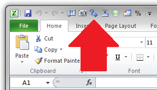 We’ve already gone over my top 10 keyboard shortcuts in Excel… I’ve even shown you how to make your own custom shortcuts, using Macro capturing and a little VBA tweaking. But even if you don’t want to dive off the deep end into custom programming, there’s still a way to make quick keyboard shortcuts for some of your most-used actions. Better yet, it’s built right in to Excel, and it’s called the Quick Access Toolbar! Learn how to customize it with your favorite shortcuts and turn them in to easy hotkeys…
What is the Quick Access Toolbar?
The Quick Access Toolbar (some call it the Quick Launch Toolbar) is a feature that was added to Excel 2007 that added an extra set of buttons above the normal menus on the Excel Ribbon. You can see it circled here:
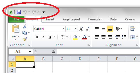
Customizing the Quick Access Toolbar
You can customize the buttons that appear on the Quick Access Toolbar by clicking the drop-down menu at the end and choosing More Commands…
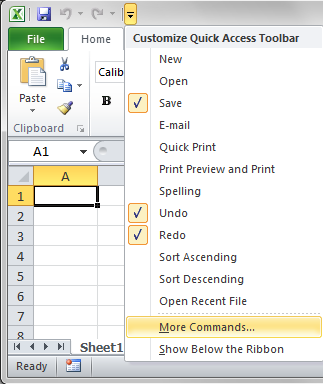
If it’s too hard to find them on the list, you can browse the menu tabs, and right-click icons you like to add them to the Quick Access Toolbar.
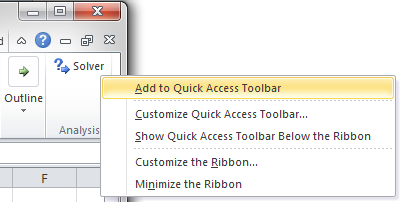
Accessing the Keyboard Shortcuts
Having a custom toolbar is great, but that’s not even the best part about the Quick Access Toolbar. The toolbar has keyboard shortcuts built in!
Press ALT and they are revealed…

In my example above, ALT+1 saves the active workbook. ALT+4 brings up the Freeze Panes dialog. ALT-6 launches Solver. You can re-arrange the order of the shortcuts to put your favorites closer to the front. All that, and no Macros or VBA in sight!
Get the latest Excel tips and tricks by joining the newsletter!
 Andrew Roberts has been solving business problems with Microsoft Excel for over a decade. Excel Tactics is dedicated to helping you master it.
Join the newsletter to stay on top of the latest articles. Sign up and you’ll get a free guide with 10 time-saving keyboard shortcuts!
Every user has different priorities and different challenges to overcome. This makes it impossible to offer all the Excel shortcuts to please everyone. But the good news is that Microsoft enables you to create your own shortcuts. You need macros for this, which make it possible to record and save a sequence of steps. When the macro is executed afterwards, the same steps will be performed automatically by Excel. The practical thing about it is that you can assign macro shortcuts and activate them quickly.
To create an Excel shortcut, first select the “Record Macro” tool, then select a name for the macro and assign a shortcut to it. You should choose a combination that isn’t already being used by Excel, otherwise the older combination will lose its original function. So, in addition to the default control key, you can also use the shift key and combine both with a letter. If you want, you can write a description with the new macro so that you can see straightaway what it does.
In this first mask, you decide how you want to save the macro. If you choose “This Workbook” or “New Workbook,” the macro and therefore also the Excel shortcut are only valid in a single folder. The best way around this is to select “Personal Macro Workbook,” meaning the macro will be available whenever you use Excel.
Once you’ve created a macro, you may need to make changes to it. The cell specifications within the function are always absolute. This means that as soon as you add another line, for example, it will no longer be taken into account by the macro. To change this, select the corresponding macro under “View Macros” and go to “Edit”. Microsoft Visual Basic for Applications (VBA) will open and this is where you can access the macro’s source code and make changes. The function for selecting the area can be found, for example, under “.SetRange.”