
Resize a table by adding or removing rows and columns
Excel for Microsoft 365 Excel for the web Excel 2021 Excel 2019 Excel 2016 Excel 2013 Excel 2010 Excel 2007 More…Less
After you create an Excel table in your worksheet, you can easily add or remove table rows and columns.
You can use the Resize command in Excel to add rows and columns to a table:
-
Click anywhere in the table, and the Table Tools option appears.
-
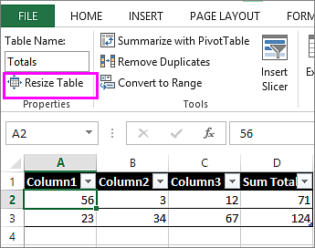
Click Design > Resize Table.

-
Select the entire range of cells you want your table to include, starting with the upper-leftmost cell.
In the example shown below, the original table covers the range A1:C5. After resizing to add two columns and three rows, the table will cover the range A1:E8.
Tip: You can also click Collapse Dialog
to temporarily hide the Resize Table dialog box, select the range on the worksheet, and then click Expand dialog . -
When you’ve selected the range you want for your table, press OK.
Add a row or column to a table by typing in a cell just below the last row or to the right of the last column, by pasting data into a cell, or by inserting rows or columns between existing rows or columns.
Start typing
-
To add a row at the bottom of the table, start typing in a cell below the last table row. The table expands to include the new row. To add a column to the right of the table, start typing in a cell next to the last table column.
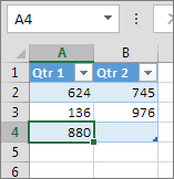
In the example shown below for a row, typing a value in cell A4 expands the table to include that cell in the table along with the adjacent cell in column B.
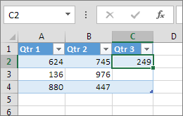
In the example shown below for a column, typing a value in cell C2 expands the table to include column C, naming the table column Qtr 3 because Excel sensed a naming pattern from Qtr 1 and Qtr 2.
Paste data
-
To add a row by pasting, paste your data in the leftmost cell below the last table row. To add a column by pasting, paste your data to the right of the table’s rightmost column.
If the data you paste in a new row has as many or fewer columns than the table, the table expands to include all the cells in the range you pasted. If the data you paste has more columns than the table, the extra columns don’t become part of the table—you need to use the Resize command to expand the table to include them.
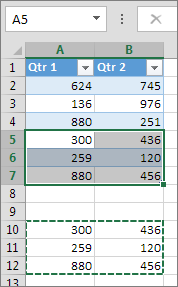
In the example shown below for rows, pasting the values from A10:B12 in the first row below the table (row 5) expands the table to include the pasted data.
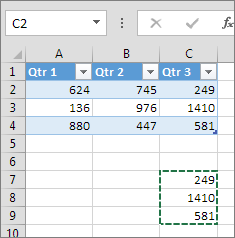
In the example shown below for columns, pasting the values from C7:C9 in the first column to right of the table (column C) expands the table to include the pasted data, adding a heading, Qtr 3.
Use Insert to add a row
-
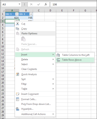
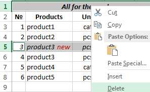
To insert a row, pick a cell or row that’s not the header row, and right-click. To insert a column, pick any cell in the table and right-click.
-
Point to Insert, and pick Table Rows Above to insert a new row, or Table Columns to the Left to insert a new column.
If you’re in the last row, you can pick Table Rows Above or Table Rows Below.
In the example shown below for rows, a row will be inserted above row 3.
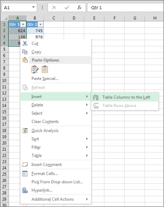
For columns, if you have a cell selected in the table’s rightmost column, you can choose between inserting Table Columns to the Left or Table Columns to the Right.
In the example shown below for columns, a column will be inserted to the left of column 1.
-
Select one or more table rows or table columns that you want to delete.
You can also just select one or more cells in the table rows or table columns that you want to delete.
-
On the Home tab, in the Cells group, click the arrow next to Delete, and then click Delete Table Rows or Delete Table Columns.
You can also right-click one or more rows or columns, point to Delete on the shortcut menu, and then click Table Columns or Table Rows. Or you can right-click one or more cells in a table row or table column, point to Delete, and then click Table Rows or Table Columns.
Just as you can remove duplicates from any selected data in Excel, you can easily remove duplicates from a table.
-
Click anywhere in the table.
This displays the Table Tools, adding the Design tab.
-
On the Design tab, in the Tools group, click Remove Duplicates.
-
In the Remove Duplicates dialog box, under Columns, select the columns that contain duplicates that you want to remove.
You can also click Unselect All and then select the columns that you want or click Select All to select all of the columns.
Note: Duplicates that you remove are deleted from the worksheet. If you inadvertently delete data that you meant to keep, you can use Ctrl+Z or click Undo  on the Quick Access Toolbar to restore the deleted data. You may also want to use conditional formats to highlight duplicate values before you remove them. For more information, see Add, change, or clear conditional formats.
-
Make sure that the active cell is in a table column.
-
Click the arrow
in the column header. -
To filter for blanks, in the AutoFilter menu at the top of the list of values, clear (Select All), and then at the bottom of the list of values, select (Blanks).
Note: The (Blanks) check box is available only if the range of cells or table column contains at least one blank cell.
-
Select the blank rows in the table, and then press CTRL+- (hyphen).
You can use a similar procedure for filtering and removing blank worksheet rows. For more information about how to filter for blank rows in a worksheet, see Filter data in a range or table.
-
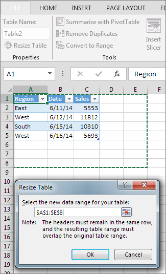
Select the table, then select Table Design > Resize Table.
-
Adjust the range of cells the table contains as needed, then select OK.
Important: Table headers can’t move to a different row, and the new range must overlap the original range.
Need more help?
You can always ask an expert in the Excel Tech Community or get support in the Answers community.
See Also
How can I merge two or more tables?
Create an Excel table in a worksheet
Use structured references in Excel table formulas
Format an Excel table
Need more help?
![]()
Download Article
![]()
Download Article
Do you have a table in Excel that you need to add more data to, like an outdated grade sheet? This wikiHow will teach you how to add a row to a table in Excel using the «Resize Table» setting for Windows, the web version, and Mac.
-
1
Open your project in Excel. Double-click your .xls worksheet file in File Explorer. Alternatively, right-click the file and select Open with > Excel.
- If you already have Excel open, go to File > Open and open your project.
-
2
Click anywhere in the table. Once you click the table, you’ll see «Table Tools» are listed as your current tab at the top of the editing space.
Advertisement
-
3
Click Design. It’s in the menu near the top of your screen.
-
4
Click Resize Table. This icon is listed in the «Properties» grouping to the far left in the menu.
-
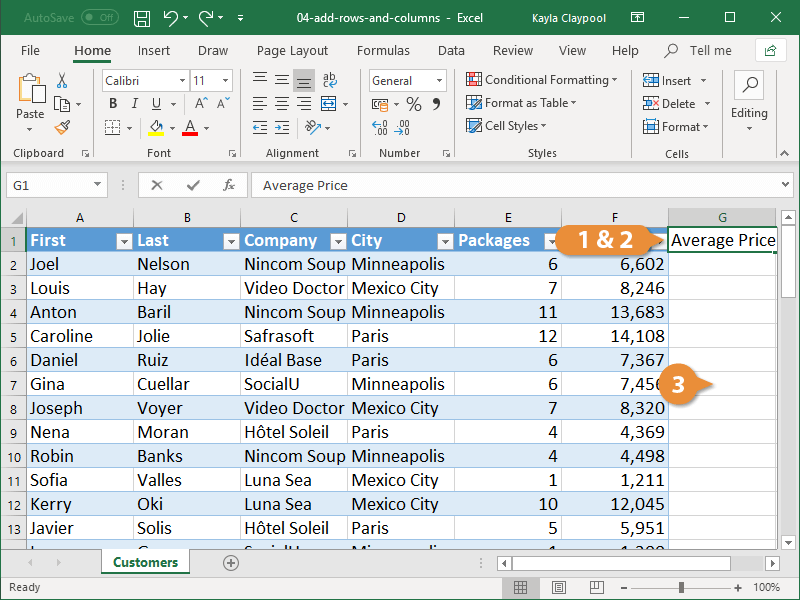
5
Select the new range of rows and columns you want to use in the table. Start with the upper-left cell of your table, and end with the bottom-right cell, which means you can add rows at the bottom of the table. Your original data set will highlight in blue. Your new selection will be outlined with a dashed border.
- Added rows must be below your table so they can be added.
-
6
Click OK. Once you’ve selected the new rows to include in the table, select OK in the dialog window to close it.[1]
- You can also insert a row or column in the middle of the table by right-clicking a cell in your data, selecting Insert and Table Columns to the Left/Right or Table Rows Above/Below.


Advertisement
-
1
Open your project in Excel. Double-click your .xls worksheet file in Finder or right-click the file and select Open with > Excel.
- If you already have Excel open, go to File > Open and open your project.
-
2
Right-click your table. A menu will appear at your cursor.
-
3
Hover your mouse over Insert and click Table Rows Above. You’ll be able to specify how many rows you want to add to the table in the next step.
- If hovering your mouse over the option doesn’t work, click it, then select Shift cells down.
-
4
Enter how many rows you want to add and press ⏎ Return. The rows will be added to the bottom of your table.[2]
- You can also insert a row or column in the middle of the table by right-clicking a cell in your data, selecting Insert and Table Columns to the Left/Right or Table Rows Above/Below.


Advertisement
-
1
Go to https://www.office.com/, login, and launch Excel. Once you navigate to the login site and enter your Microsoft account information, you’ll be logged in. Finally, launch Excel.
-
2
Click a project to open it. You’ll also see all the projects you have saved to OneDrive.
-
3
Click anywhere in the table. Once you click the table, you’ll see «Table Design» as an option in the editing ribbon above your spreadsheet document.
-
4
Click the Table Design tab and select Resize Table. The «Resize» option is all the way to the left of the menu in the «Table Design» tab.
-
5
Enter the new range for your table. For example, if you want to add one row, just increase the last number: If your current data set for the table is A1 to H13, input A1:H14 to add a row at the bottom of the table.
-
6
Click OK. This will close the window and change the range of the table.
- You can also insert a row or column in the middle of the table by right-clicking a cell in your data, selecting Insert and Table Columns to the Left/Right or Table Rows Above/Below.


Advertisement
Ask a Question
200 characters left
Include your email address to get a message when this question is answered.
Submit
Advertisement
Thanks for submitting a tip for review!
References
About This Article
Article SummaryX
1. Open your project in Excel.
2. Click anywhere in the table.
3. Click Design.
4. Click Resize Table.
5. Enter the new range of rows and columns you want to use in the table.
6. Click Ok.
Did this summary help you?
Thanks to all authors for creating a page that has been read 12,779 times.
Is this article up to date?
See all How-To Articles
This tutorial demonstrates how to add rows to a table in Excel and Google Sheets.
Add Rows to the Bottom of a Table
If your data is formatted as an Excel table, it is easy to add extra rows.
Add Rows With the Tab Key
- Click in the bottom right-hand corner of your formatted table, in the last available cell.
- Press TAB to add another row to your table.
Add Rows by Typing in the Next Row
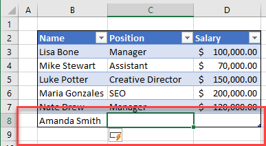
A row is also added to a formatted Excel table when you type in the first cell of the first blank row at the end of your table.
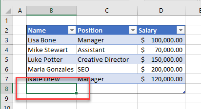
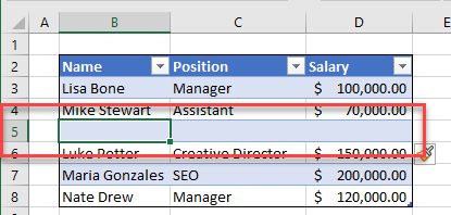
- Click in the first cell of the row below your table.

- Type in a value, and then press TAB.
- When you do this, a menu button appears. Click on the menu to see the options available.
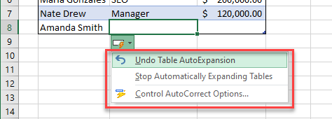
- If you DO NOT want the new row to be automatically included in the table, click Undo Table AutoExpansion.
- If you want to stop this table, and any future tables from automatically expanding, click Stop Automatically Expanding Tables.
- To view more AutoCorrect options, click Control AutoCorrect Options.
Add Rows in the Middle of a Table
Add Rows With the Ribbon
- Click in the row of your Excel table where you want the new row to be inserted.

- In the Ribbon, select Home > Insert > Insert Table Rows Above.
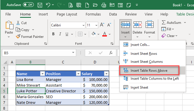
- A new row is added above the row that is currently selected in your table.
Add Rows With the Keyboard
- Click in the row of your Excel table where you want the new row to be inserted.
- Press and hold CTRL, then press the + sign to insert a row above your selected row.
Resize a Table
You can also add rows to an existing table by resizing the table.
- Position your mouse at the small handle in the bottom right-hand corner of the table. Your mouse pointer changes to a small double-headed black arrow.
![]()
- Drag the mouse down the number of rows to be inserted.
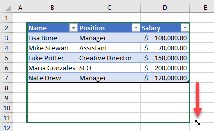
- Release the mouse to add the rows to your table.
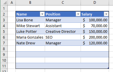
Note: You can also drag back up again to delete the rows!
Add Rows to a Table in Google Sheets
Add a Row to the Bottom of a Table
If your table in Google Sheets has been formatted with alternating colors (Menu > Format > Alternating Colors), you can automatically add rows to the formatted table.
- Click in the cell below the last row of your table.
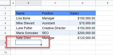
- Type in your data, and then press TAB.
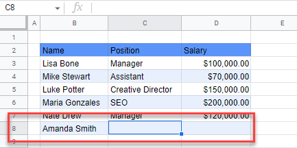
- A new row is added formatted in the style you have chosen for your table.
Add a Row in the Middle of a Table
- Click in the middle of your table where you want the row inserted.
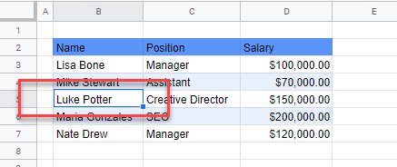
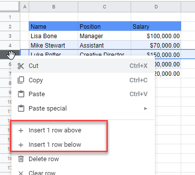
- On the row header, right click to obtain the quick menu.
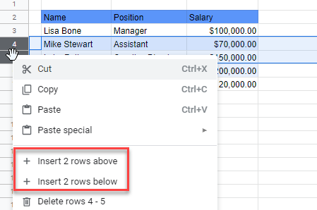
Tip: By selecting more than one row in your table, the quick menu changes accordingly. So, if you select two rows, the menu is shown as in the picture below:
- Select the option to add the row or rows to your table.
Even after a table is created, you can add additional rows and columns. Whether you add new cells within the current range or adjacent to the table, they will automatically be formatted to match the current table style.
When a formula is entered in a blank column of a table, the formula automatically fills the rest of the column, without using the AutoFill feature. If rows are added to the column, the formula appears in those rows as well.
Insert options aren’t available if you select a column header.
- Insert Table Rows Above: Inserts a new row above the select cell.
- Insert Table Columns to the Left: Inserts a new column to the left of the selected cell.
Right-click a row or column next to where you want to add data, point to Insert in the menu, and select an insertion option.
Delete Rows and Columns
You can also remove unwanted table rows and columns by deleting them.
- Select a cell in the row or column you want to delete.
- Click the Delete list arrow.
- Select Delete Table Rows or Delete Table Columns.
Right-click the row or column you want to delete, point to Delete in the menu, and select Table Columns or Table Rows.
The selected row(s) or column(s) and all the data in them are deleted.
FREE Quick Reference
Free to distribute with our compliments; we hope you will consider our paid training.
Источник
How to insert a row or a column in Excel
Creating new tables, reports and pricelists of different types, we cannot predict the number of necessary rows and columns. Using Excel program implies to a great extent creating and setting up spreadsheets, which requires inserting and deleting different elements.
First, let’s consider the methods of inserting sheet rows and columns when creating spreadsheets.
Note that in this tutorial we indicate hot keys for adding or deleting rows and columns. They should be used after highlighting the whole row or column. To highlight the row where the cursor is placed, press the combination of hot keys: SHIFT+SPACEBAR. Hot keys for highlighting a column are CTRL+SPACEBAR.
How to insert a column between other columns?
Assuming you have a pricelist lacking line item numbering:
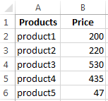
To insert a column between other columns for filling in pricelist items numbering you can use one of the two ways:
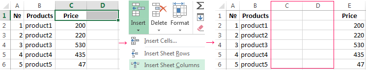
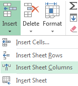
- Move the cursor to activate A1 cell. Then go to tab «HOME», tool section «Cells» and click «Insert», in the popup menu select «Insert Sheet Columns» option.
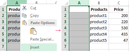
- Right-click the heading of column A. Select «Insert» option on the shortcut menu.
- Select the column, and press the hotkey combination CTRL+SHIFT+PLUS.
Now you can type the numbers of pricelist line items.
Simultaneous insertion of several columns
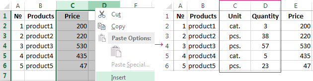
The pricelist still lacks two columns: quantity and units (items, kilograms, liters, packs). To add simultaneously, highlight the two-cell range (C1:D1). Then use the same tool on the «Insert»-«Insert Sheet Columns» main tab.
Alternatively, highlight two headings of columns C and D, right-click and select «Insert» option.
Note. Columns are always added to the left side. There appear as many new columns as many old ones have been highlighted. The order of inserted also depends on the order of highlighting. For example, next but one etc.
How to insert a row between rows in Excel?
Now let’s add a heading and a new goods line item «All for the garden» to the pricelist. To this end, let’s insert two new rows simultaneously.
Highlight the nonadjacent range of two cells A1,A4 (note that character “,” is used instead of character “:” – it means that two nonadjacent ranges should be highlighted; to make sure, type A1; A4 in the name field and press Enter). You know from the previous tutorials how to highlight nonadjacent ranges.
Now once again use the tool «HOME»-«Insert»-«Insert Sheet Columns». The picture shows how to insert a blank row between other rows in Excel.
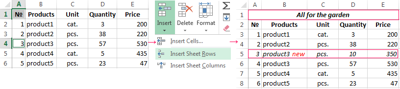
It is easy to guess the second way. You need to highlight headings of rows 1 and 3, right-click on one of the highlighted rows and select «Insert» option.
To add a row or a column in Excel use hot keys CTRL+SHIFT+PLUS having highlighted the appropriate row or column.
Note. New rows are always added above the highlighted rows.
Deleting rows and columns
When working with Excel you need to delete rows and columns as often as to insert them. Therefore, you have to practice.
By way of illustration, let’s delete from our pricelist the numbering of goods line items and the unit column simultaneously.
Highlight the nonadjacent range of cells A1; D1 and select «HOME»-«Delete»-«Delete Sheet Rows». The shortcut menu can also be used for deleting if you highlight headings A1 and D1 instead of cells.
Row deleting is performed in the similar way. You only need to select a tool in the appropriate menu. Applying a shortcut menu is the same. You only have to highlight the rows correspondingly by row numbers.
To delete a row or a column in Excel, use hot keys CTRL+MINUS having preliminary highlighted them.
Note. Inserting new columns and rows is in fact substitution, as the number of rows (1 048 576) and columns (16 384) doesn’t change. The new just replace the old ones. You should consider this fact when filling in the sheet with data by more than 50% — 80%.
Источник
Resize a table by adding or removing rows and columns
After you create an Excel table in your worksheet, you can easily add or remove table rows and columns.
You can use the Resize command in Excel to add rows and columns to a table:
Click anywhere in the table, and the Table Tools option appears.
Click Design > Resize Table.
Select the entire range of cells you want your table to include, starting with the upper-leftmost cell.
In the example shown below, the original table covers the range A1:C5. After resizing to add two columns and three rows, the table will cover the range A1:E8.
Tip: You can also click Collapse Dialog  to temporarily hide the Resize Table dialog box, select the range on the worksheet, and then click Expand dialog
  .
.
When you’ve selected the range you want for your table, press OK.
Add a row or column to a table by typing in a cell just below the last row or to the right of the last column, by pasting data into a cell, or by inserting rows or columns between existing rows or columns.
To add a row at the bottom of the table, start typing in a cell below the last table row. The table expands to include the new row. To add a column to the right of the table, start typing in a cell next to the last table column.
In the example shown below for a row, typing a value in cell A4 expands the table to include that cell in the table along with the adjacent cell in column B.
In the example shown below for a column, typing a value in cell C2 expands the table to include column C, naming the table column Qtr 3 because Excel sensed a naming pattern from Qtr 1 and Qtr 2.
To add a row by pasting, paste your data in the leftmost cell below the last table row. To add a column by pasting, paste your data to the right of the table’s rightmost column.
If the data you paste in a new row has as many or fewer columns than the table, the table expands to include all the cells in the range you pasted. If the data you paste has more columns than the table, the extra columns don’t become part of the table—you need to use the Resize command to expand the table to include them.
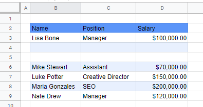
In the example shown below for rows, pasting the values from A10:B12 in the first row below the table (row 5) expands the table to include the pasted data.
In the example shown below for columns, pasting the values from C7:C9 in the first column to right of the table (column C) expands the table to include the pasted data, adding a heading, Qtr 3.
Use Insert to add a row
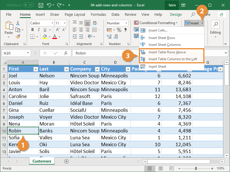
To insert a row, pick a cell or row that’s not the header row, and right-click. To insert a column, pick any cell in the table and right-click.
Point to Insert, and pick Table Rows Above to insert a new row, or Table Columns to the Left to insert a new column.
If you’re in the last row, you can pick Table Rows Above or Table Rows Below.
In the example shown below for rows, a row will be inserted above row 3.
For columns, if you have a cell selected in the table’s rightmost column, you can choose between inserting Table Columns to the Left or Table Columns to the Right.
In the example shown below for columns, a column will be inserted to the left of column 1.
Select one or more table rows or table columns that you want to delete.
You can also just select one or more cells in the table rows or table columns that you want to delete.
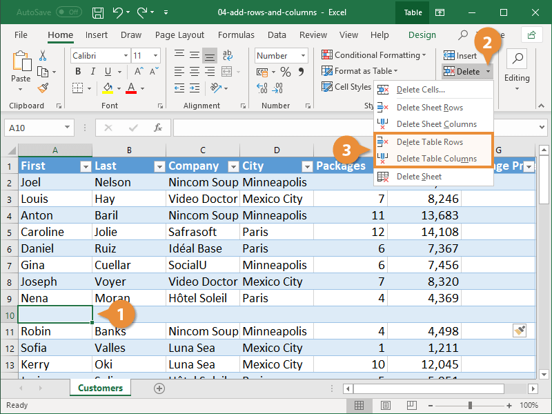
On the Home tab, in the Cells group, click the arrow next to Delete, and then click Delete Table Rows or Delete Table Columns.

You can also right-click one or more rows or columns, point to Delete on the shortcut menu, and then click Table Columns or Table Rows. Or you can right-click one or more cells in a table row or table column, point to Delete, and then click Table Rows or Table Columns.
Just as you can remove duplicates from any selected data in Excel, you can easily remove duplicates from a table.
Click anywhere in the table.
This displays the Table Tools, adding the Design tab.
On the Design tab, in the Tools group, click Remove Duplicates.
In the Remove Duplicates dialog box, under Columns, select the columns that contain duplicates that you want to remove.
You can also click Unselect All and then select the columns that you want or click Select All to select all of the columns.
Note: Duplicates that you remove are deleted from the worksheet. If you inadvertently delete data that you meant to keep, you can use Ctrl+Z or click Undo on the Quick Access Toolbar to restore the deleted data. You may also want to use conditional formats to highlight duplicate values before you remove them. For more information, see Add, change, or clear conditional formats.
Make sure that the active cell is in a table column.
Click the arrow  in the column header.
To filter for blanks, in the AutoFilter menu at the top of the list of values, clear (Select All), and then at the bottom of the list of values, select (Blanks).
Note: The (Blanks) check box is available only if the range of cells or table column contains at least one blank cell.
Select the blank rows in the table, and then press CTRL+- (hyphen).
You can use a similar procedure for filtering and removing blank worksheet rows. For more information about how to filter for blank rows in a worksheet, see Filter data in a range or table.
Select the table, then select Table Design > Resize Table.
Adjust the range of cells the table contains as needed, then select OK.
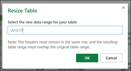
Important: Table headers can’t move to a different row, and the new range must overlap the original range.
Need more help?
You can always ask an expert in the Excel Tech Community or get support in the Answers community.
Источник

Even after a table is created, you can add additional rows and columns. Whether you add new cells within the current range or adjacent to the table, they will automatically be formatted to match the current table style.
Insert a Row or Column Adjacent to the Table
- Click in a blank cell next to the table.
- Type a cell value.
- Click anywhere outside the cell or press the Enter key to add the value.

The new row or column is added to the table and the table formatting is applied.
When a formula is entered in a blank column of a table, the formula automatically fills the rest of the column, without using the AutoFill feature. If rows are added to the column, the formula appears in those rows as well.
Insert a Row or Column within a Table
- Select a cell in the table row or column next to where you want to add the row or column.
Insert options aren’t available if you select a column header.
- Click the Insert list arrow on the Home tab.
- Select an insert table option.
- Insert Table Rows Above: Inserts a new row above the select cell.
- Insert Table Columns to the Left: Inserts a new column to the left of the selected cell.
Right-click a row or column next to where you want to add data, point to Insert in the menu, and select an insertion option.
Delete Rows and Columns
You can also remove unwanted table rows and columns by deleting them.
- Select a cell in the row or column you want to delete.
- Click the Delete list arrow.
- Select Delete Table Rows or Delete Table Columns.
Right-click the row or column you want to delete, point to Delete in the menu, and select Table Columns or Table Rows.
The selected row(s) or column(s) and all the data in them are deleted.
FREE Quick Reference
Click to Download
Free to distribute with our compliments; we hope you will consider our paid training.
To insert multiple rows in Excel, we must first select the number of rows. Then, based on that, we can insert those rows. Once the rows are inserted, we can use the F4 key to repeat the last action and insert as many rows as needed.
Table of contents
- How to Insert Multiple Rows in Excel?
- Top 4 Useful Methods to Insert Rows in Excel (Discussed with an Example)
- Method #1 – Using INSERT option
- Method #2 – Using Excel Short Cut (Shift+Space Bar)
- Method 3: Using the Name Box.
- Method 4: Using the Copy & Paste Method
- Alternative Coolest Technique
- Things to Remember
- Recommended Articles
- Top 4 Useful Methods to Insert Rows in Excel (Discussed with an Example)
Top 4 Useful Methods to Insert Rows in Excel (Discussed with an Example)
- Insert Row using INSERT Option
- Insert Multiple Rows in Excel using Short Cut Key (Shift+Space Bar)
- Insert Multiple Rows Using the Name Box
- Insert Multiple Rows Using the Copy & Paste Method
Let us Discuss each method in detail along with an example –
You can download this Insert Multiple Rows Excel Template here – Insert Multiple Rows Excel Template
Method #1 – Using INSERT option
We need to select the row first, but it depends on how many rows we insert. For example, if we want to insert two rows, we need to select two rows. If we need to insert three multiple rows, we need to choose three rows, and so on.
In the above image, we have selected three rows, and now we will right-click on the column header and click on “Insert.” It would insert three multiple rows in a single shot.
Method #2 – Using Excel Short Cut (Shift+Space Bar)
Below are the steps to insert rows in Excel using the Excel shortcut (Shift + Spacebar).
- We must first select the cell above which we want to insert the row.

- We must use the shortcut key to select the entire row instantly. The shortcut keyboard key is “Shift + Spacebar.”

- If we want to insert two to three rows, select those many rows by using the “Shift + Down Arrow” key. In the below image, we have chosen four rows.

- Now, we must click on another keyboard “Ctrl + “(plus key) shortcut key to insert a row in Excel.

Now we have inserted four multiple rows. Suppose we need to insert another Four rows; Click on Ctrl + if the rows are selected, or instead, we can use the key F4, which repeats the previous action in excel.


Method 3: Using the Name Box.
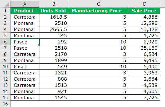
Suppose we need to insert 150 rows above the cell we have selected. It will take some time because we need to choose those many rows first and then insert them using the Excel shortcut.
Selecting 150 rows instantly is not possible in the above two methods. We can select those name box in excel.In Excel, the name box is located on the left side of the window and is used to give a name to a table or a cell. The name is usually the row character followed by the column number, such as cell A1.read more
- Step 1: Select the cell above we need to insert rows.
- Step 2: We must mention the row range on the name box. We have mentioned 5:155 because we have to insert 150 rows in this case.
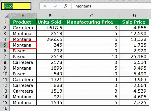
- Step 3: After typing the range, hit the enter key; this will select the cells from 5:155 instantly.
- Step 4: Once the range is selected, we must use the “Ctrl +” shortcut key to insert a row in Excel. It will insert 150 rows in just a click.
Alternative Shortcut Key to Insert Row in Excel: ALT + H + I + R is another shortcut key to insert a row in Excel.

Method 4: Using the Copy & Paste Method
Microsoft Excel is so flexible. For example, can you believe we can insert rows by copy-paste?
Yes! You heard it right. We can insert rows just by copying and pasting another blank row.
- Step 1: Select the blank row and copy.

- Step 2: Now select the cell above you want to insert rows.
- Step 3: Once the desired cell is selected, select the number of rows you wish to insert and right-click and choose Insert Copied Cells.

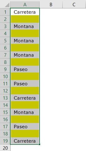
Case Study: I have data from A1: A10, as shown in the below image.
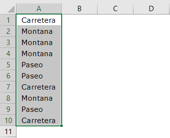
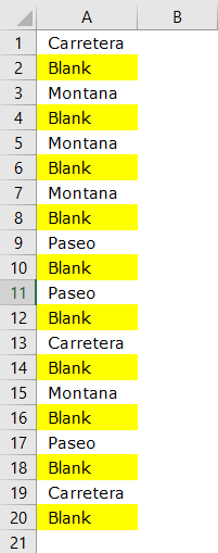
We want to insert one blank row after every row, as shown in the below image.
Alternative Coolest Technique
In the above example, we have only ten rows. What if we have to do it for 100 cells? It will take a lot of time. However, we have the coolest technique you have ever seen.
Follow the below steps to learn.
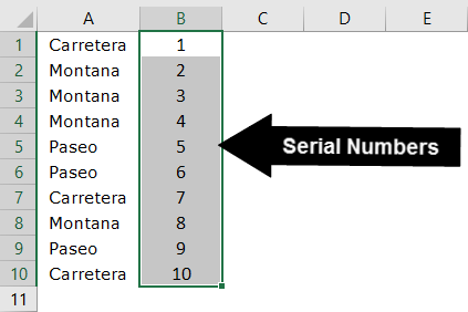
- Step 1: First, Insert serial numbers next to the data.
- Step 2: Copy those serial numbers and paste them after the last serial number.
- Step 3: Now, select the entire data, including serial numbers, and press Alt + D + S.
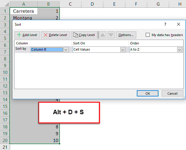
- Step 4: Select the second column from the dropdown list and ensure the smallest to highest is selected.

- Step 5: Now, click on the Ok. This would instantly insert the blank row after every row.
Amazing. Probably the coolest and the most intelligent technique you have learned to date.
Things to Remember
- The shortcut key to insert a row in excel is “Alt + H + I + R, Ctrl +.”
- We must always insert new rows after selecting the entire row (s) first. Otherwise, there are chances that the data may shuffle.
Recommended Articles
This article is a guide to Insert Multiple Rows in Excel. Here, we learn to insert multiple rows in Excel using Excel insert shortcuts, Excel examples, and downloadable Excel templates. You may also look at these useful functions in Excel: –
- Count Rows in ExcelThere are numerous ways to count rows in Excel using the appropriate formula, whether they are data rows, empty rows, or rows containing numerical/text values. Depending on the circumstance, you can use the COUNTA, COUNT, COUNTBLANK, or COUNTIF functions.read more
- VBA Insert RowTo insert rows we use worksheet method with the insert command to insert a row, we also provide a row reference where we want to insert another row similar to the columns.read more
- Copy Paste in VBAIn VBA, we use the copy method with range property to copy a value from one cell to another. To paste the value, we use the worksheet function paste exceptional or paste method.read more
- Insert Row Shortcut in ExcelThe insertion of an excel row is simply the addition of a new (blank) row to the worksheet. The insertion of a row is eased with the help of shortcuts.read more
- Break Links in ExcelIn the excel worksheet, there are two different methods to break external links. The first method is to copy and paste as a value method, and the second method is to go to the DATA tab, click Edit Links, and choose the break the link option.read more
Creating new tables, reports and pricelists of different types, we cannot predict the number of necessary rows and columns. Using Excel program implies to a great extent creating and setting up spreadsheets, which requires inserting and deleting different elements.
First, let’s consider the methods of inserting sheet rows and columns when creating spreadsheets.
Note that in this tutorial we indicate hot keys for adding or deleting rows and columns. They should be used after highlighting the whole row or column. To highlight the row where the cursor is placed, press the combination of hot keys: SHIFT+SPACEBAR. Hot keys for highlighting a column are CTRL+SPACEBAR.
How to insert a column between other columns?
Assuming you have a pricelist lacking line item numbering:
To insert a column between other columns for filling in pricelist items numbering you can use one of the two ways:
- Move the cursor to activate A1 cell. Then go to tab «HOME», tool section «Cells» and click «Insert», in the popup menu select «Insert Sheet Columns» option.
- Right-click the heading of column A. Select «Insert» option on the shortcut menu.
- Select the column, and press the hotkey combination CTRL+SHIFT+PLUS.
Now you can type the numbers of pricelist line items.
Simultaneous insertion of several columns
The pricelist still lacks two columns: quantity and units (items, kilograms, liters, packs). To add simultaneously, highlight the two-cell range (C1:D1). Then use the same tool on the «Insert»-«Insert Sheet Columns» main tab.
Alternatively, highlight two headings of columns C and D, right-click and select «Insert» option.
Note. Columns are always added to the left side. There appear as many new columns as many old ones have been highlighted. The order of inserted also depends on the order of highlighting. For example, next but one etc.
How to insert a row between rows in Excel?
Now let’s add a heading and a new goods line item «All for the garden» to the pricelist. To this end, let’s insert two new rows simultaneously.
Highlight the nonadjacent range of two cells A1,A4 (note that character “,” is used instead of character “:” – it means that two nonadjacent ranges should be highlighted; to make sure, type A1; A4 in the name field and press Enter). You know from the previous tutorials how to highlight nonadjacent ranges.
Now once again use the tool «HOME»-«Insert»-«Insert Sheet Columns». The picture shows how to insert a blank row between other rows in Excel.
It is easy to guess the second way. You need to highlight headings of rows 1 and 3, right-click on one of the highlighted rows and select «Insert» option.
To add a row or a column in Excel use hot keys CTRL+SHIFT+PLUS having highlighted the appropriate row or column.
Note. New rows are always added above the highlighted rows.
Deleting rows and columns
When working with Excel you need to delete rows and columns as often as to insert them. Therefore, you have to practice.
By way of illustration, let’s delete from our pricelist the numbering of goods line items and the unit column simultaneously.
Highlight the nonadjacent range of cells A1; D1 and select «HOME»-«Delete»-«Delete Sheet Rows». The shortcut menu can also be used for deleting if you highlight headings A1 and D1 instead of cells.
Row deleting is performed in the similar way. You only need to select a tool in the appropriate menu. Applying a shortcut menu is the same. You only have to highlight the rows correspondingly by row numbers.
To delete a row or a column in Excel, use hot keys CTRL+MINUS having preliminary highlighted them.
Note. Inserting new columns and rows is in fact substitution, as the number of rows (1 048 576) and columns (16 384) doesn’t change. The new just replace the old ones. You should consider this fact when filling in the sheet with data by more than 50% — 80%.
Содержание
- Вставка строки между строк
- Вставка строки в конце таблицы
- Создание умной таблицы
- Вопросы и ответы

При работе в программе Excel довольно часто приходится добавлять новые строки в таблице. Но, к сожалению, некоторые пользователи не знают, как сделать даже такие довольно простые вещи. Правда, нужно отметить, что у этой операции имеются и некоторые «подводные камни». Давайте разберемся, как вставить строку в приложении Microsoft Excel.
Вставка строки между строк
Нужно отметить, что процедура вставки новой строки в современных версиях программы Excel практически не имеет отличий друг от друга.
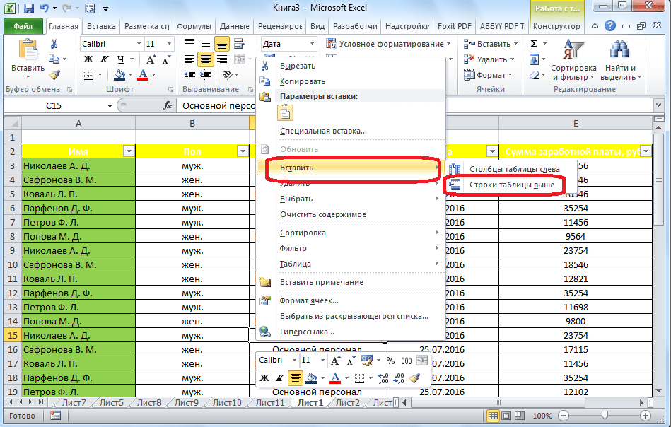
Итак, открываем таблицу, в которую нужно добавить строку. Чтобы вставить строку между строк, кликаем правой кнопкой мыши по любой ячейки строки, над которой планируем вставить новый элемент. В открывшемся контекстном меню жмем на пункт «Вставить…».
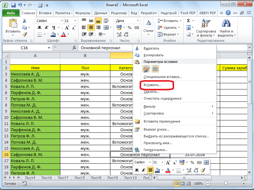
Также, существует возможность вставки без вызова контекстного меню. Для этого нужно просто нажать на клавиатуре сочетание клавиш «Ctrl+».
Открывается диалоговое окно, которое предлагает нам вставить в таблицу ячейки со сдвигом вниз, ячейки со сдвигом вправо, столбец, и строку. Устанавливаем переключатель в позицию «Строку», и жмем на кнопку «OK».
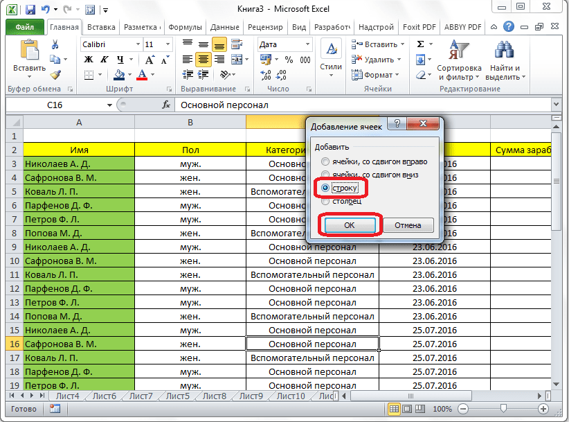
Как видим, новая строка в программе Microsoft Excel успешно добавлена.
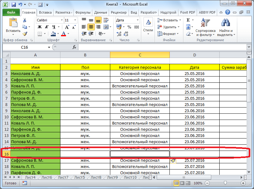
Вставка строки в конце таблицы
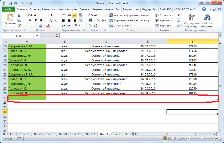
Но, что делать, если нужно вставить ячейку не между строк, а добавить строку в конце таблицы? Ведь, если применить вышеописанный метод, то добавленная строка не будет включена в состав таблицы, а останется вне её границ.
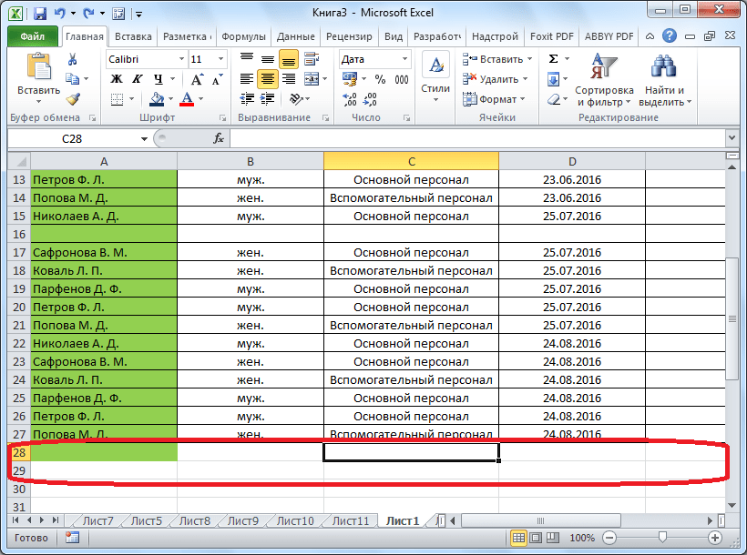
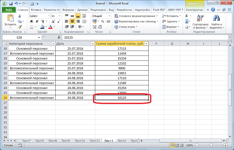
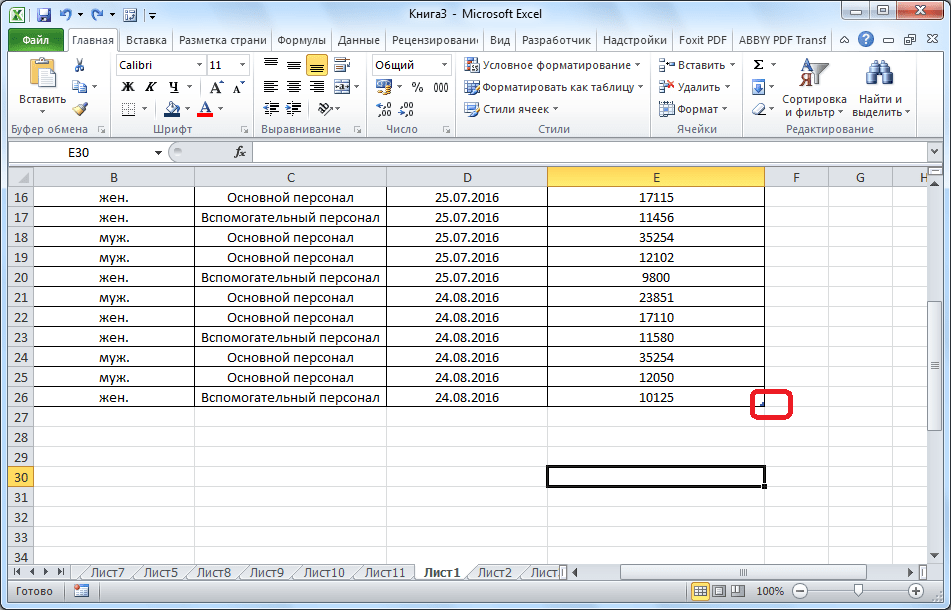
Для того, чтобы продвинуть таблицу вниз, выделяем последнюю строку таблицы. В её правом нижнем углу образовывается крестик. Тянем его вниз на столько строк, на сколько нам нужно продлить таблицу.
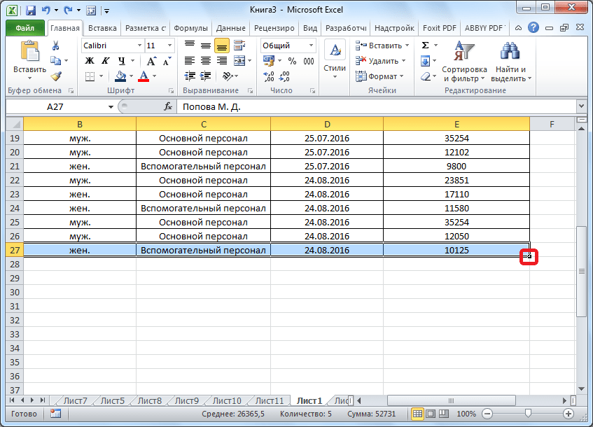
Но, как видим, все нижние ячейки формируются с заполненными данными из материнской ячейки. Чтобы убрать эти данные, выделяем новообразованные ячейки, и кликаем правой кнопкой мыши. В появившемся контекстном меню выбираем пункт «Очистить содержимое».

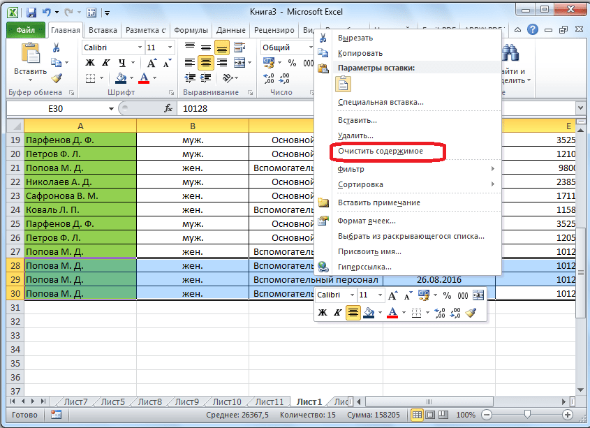
Как видим, ячейки очищены, и готовы к заполнению данными.
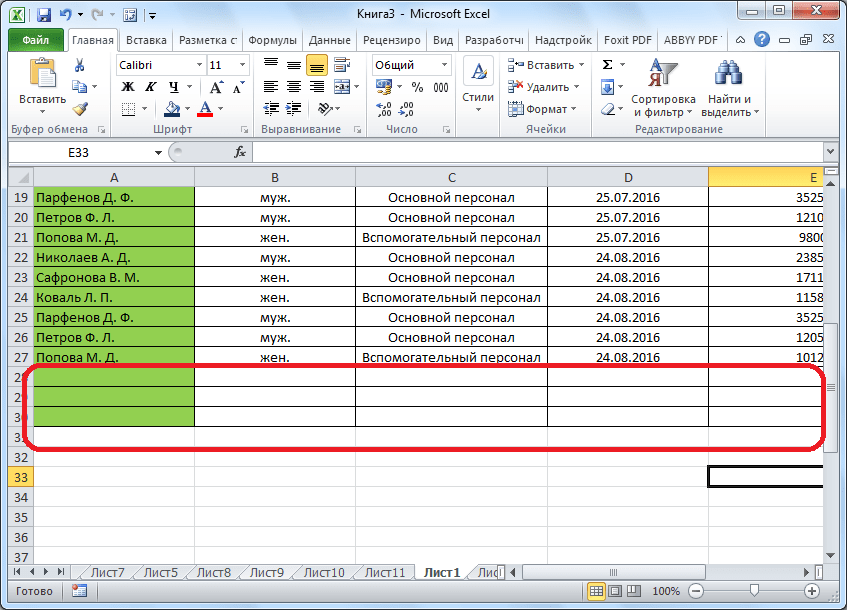
Нужно учесть, что данный способ подходит только в том случае, если в таблице нет нижней строки итогов.
Создание умной таблицы
Но, намного удобнее создать, так называемую, «умную таблицу». Это можно сделать один раз, и потом не переживать, что какая-то строка при добавлении не войдет в границы таблицы. Эта таблица будет растягиваемая, и к тому же, все данные внесенные в неё не будут выпадать из формул, применяемых в таблице, на листе, и в книге в целом.
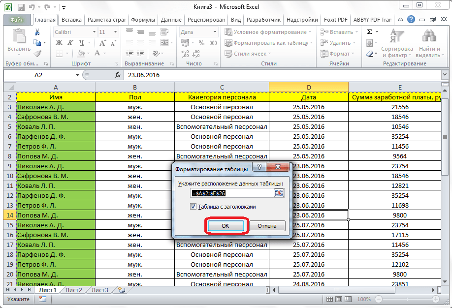
Итак, для того, чтобы создать «умную таблицу», выделяем все ячейки, которые в неё должны войти. Во вкладке «Главная» жмем на кнопку «Форматировать как таблицу». В открывшемся перечне доступных стилей выбираем тот стиль, который вы считаете для себя наиболее предпочтительным. Для создания «умной таблицы» выбор конкретного стиля не имеет значения.
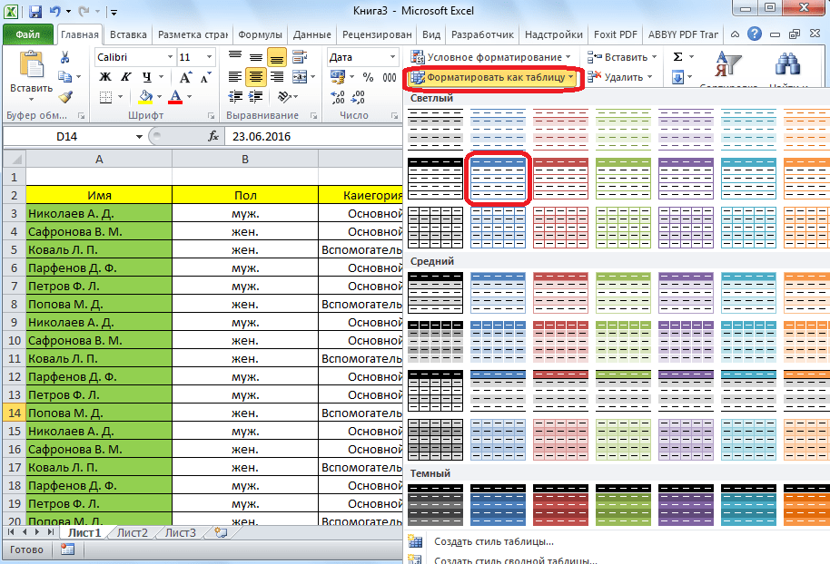
После того, как стиль выбран, открывается диалоговое окно, в котором указан диапазон выбранных нами ячеек, так что коррективы в него вносить не нужно. Просто жмем на кнопку «OK».
«Умная таблица» готова.
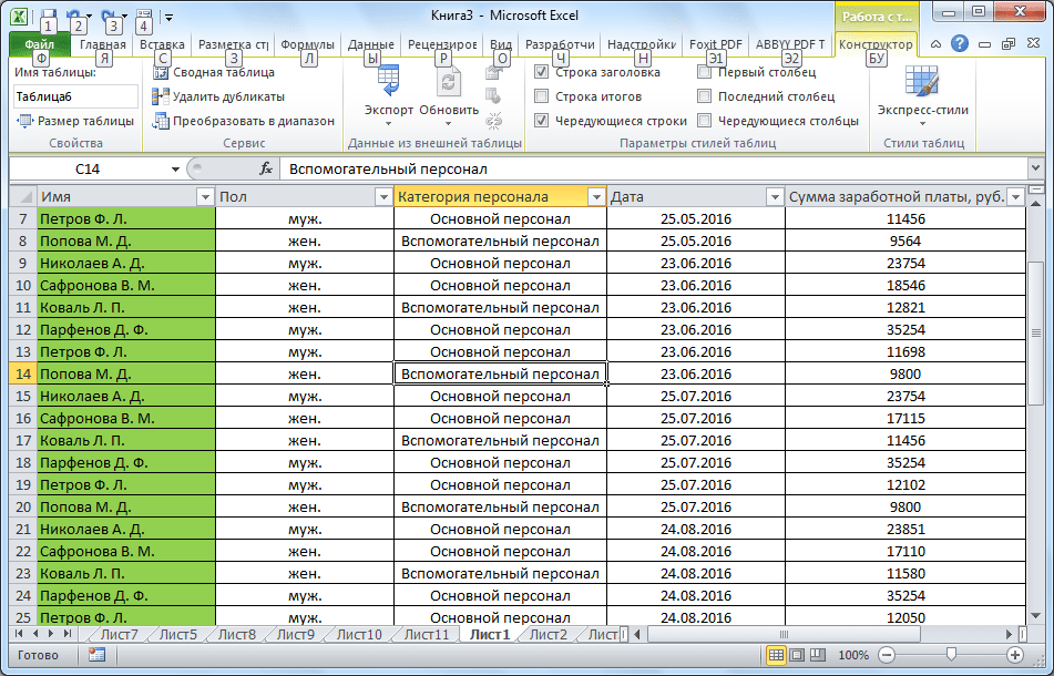
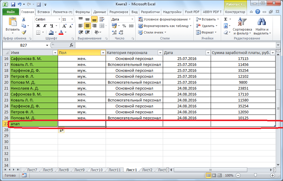
Теперь, для добавления строки, кликаем по ячейке, над которой строка будет создаваться. В контекстном меню выбираем пункт «Вставить строки таблицы выше».
Строка добавляется.
Строку между строк можно добавить простым нажатием комбинации клавиш «Ctrl+». Больше ничего на этот раз вводить не придется.
Добавить строку в конце «умной таблицы» можно несколькими способами.
Можно встать на последнюю ячейку последней строки, и нажать на клавиатуре функциональную клавишу табуляции (Tab).
Также, можно встать курсором на правый нижний угол последней ячейки, и потянуть его вниз.
На этот раз, новые ячейки будут образовываться незаполненными изначально, и их не нужно будет очищать от данных.
А можно, просто ввести любые данные под строкой ниже таблицы, и она автоматически будет включена в состав таблицы.
Как видим, добавить ячейки в состав таблицы в программе Microsoft Excel можно различными способами, но, чтобы не возникало проблем с добавлением, прежде, лучше всего, с помощью форматирования создать «умную таблицу».
![]()
When you create a table in Microsoft Excel, you might need to adjust its size later. If you need to add or remove columns or rows in a table after you create it, you have several ways to do both.
Use the Resize Table Feature in Excel
If you want to work with both tables and columns, whether adding or deleting them, the handiest way is with the Resize Table feature.
Select any cell within the table. Go to the Table Design tab that appears and click “Resize Table” on the left side of the ribbon.

In the pop-up window, you can use the cell range text box to adjust the cell references. If you prefer, you can drag through the columns and rows while the window is open. Click “OK” when you have the table sized as you want it.
If you simply want to add more columns or rows, there are a few ways to do it. You can use whichever method is most convenient or comfortable for you.
Type Data in the Next Column or Row
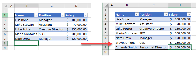
To add another column, type your data in the cell to the right of the last column. To add another row, type data in the cell below the last row. Hit Enter or Return.
This automatically adds a column or row that’s included in the table.
Paste Data in the Next Column or Row
Like typing into the cell, you can also paste data. So if you have data from another location on your clipboard, head to the cell to the right of the last column or below the last row and paste it. You can use “Paste” on the Home tab or right-click and select “Paste.”
This also adds the number of columns or rows of data, which are then part of the table.
Use the Insert Feature
Whether you like to right-click or use the buttons in the ribbon, there’s an Insert option that makes adding columns or rows easy. And like many other tasks, there are a few different ways to use Insert.
- Select a column or row, right-click, and pick “Insert.” This inserts a column to the left or in the row above.
- Select a column or row, go to the Home tab, and click “Insert” in the Cells section of the ribbon. You can also click the arrow next to the Insert button and choose “Insert Sheet Columns” or “Insert Sheet Rows.” Both options insert a column to the left or in the row above.
- Select any cell in the table, right-click, and move to “Insert.” Select “Table Columns to the Left” or “Table Rows Above” in the pop-out menu to add one or the other.
Delete Columns or Rows in an Excel Table
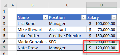
Like adding columns or rows to a table in Microsoft Excel, deleting them is just as simple. And as you’ve probably already guessed, there’s more than one way to do it! Here, you’ll simply use the Delete feature.
As you might have noticed when using the Insert feature above, there’s also a Delete option nearby. So, use one of these actions to delete a column or row.
- Select a column or row, right-click, and pick “Delete.”
- Select a column or row, go to the Home tab, and click “Delete” in the Cells section of the ribbon. Alternatively, you can click the arrow next to the Delete button and choose “Delete Sheet Columns” or “Delete Sheet Rows.”
- Select a cell in the column or row that you want to remove. Right-click, move to “Delete,” and select “Table Columns” or “Table Rows” in the pop-out menu to remove one or the other.
If you’re interested in getting help with columns and rows in Excel outside of tables, take a look at how to freeze and unfreeze columns and rows or how to convert a row to a column.
READ NEXT
- › How to Edit a Drop-Down List in Microsoft Excel
- › How to Remove Blank Rows in Excel
- › How to Remove a Table in Microsoft Excel
- › How to Insert a Total Row in a Table in Microsoft Excel
- › How to Delete a Sheet in Microsoft Excel
- › How to Create a Project Timeline in Microsoft Excel
- › How to Insert Multiple Rows in Microsoft Excel
- › Mozilla Wants Your Feature Suggestions for Thunderbird
How-To Geek is where you turn when you want experts to explain technology. Since we launched in 2006, our articles have been read billions of times. Want to know more?