
Excel concatenate() is seriously crippled, it can add 2 or more strings together, as long as they are supplied as separate parameters. This means, when you have a range of cells with text which you want to add up to create a large text, you need to write an ugly looking biggish concatenate() or use ‘&’ operator over and again.
I felt bored enough the other day to write a better concatenate(), one that can accept a range as input and output one text with all the contents of the input range. What more you can use this to delimit the input range with your own favorite character.
For example, if each of the 7 cells in a1:a7 have “a”, “b”, “c”, “d”, “e”, “f”, “g”, if you want to add all of them up using concatenate you would have to write concatenate(a1,a2,a3,a4,a5,a6,a7) which can be painful if you are planning to do this over a large range or something.
Instead, you can use concat(a1:a7) by installing the UDF (User defined function) I have written. Its nothing miraculous or anything, it just does the dirty job of going through the range for you. If you want to delimit the input range with a comma just use concat(a1:a7,",") to get the out of a,b,c,d,e,f,g Just download the concat() UDF excel add-in and double click on it to install it. If you are little weary of installing UDFs / Macros from third parties, copy past the below excel code in a new sheet’s VB editor and save the sheet as an excel addin (.xla extension)
Added on Aug 26, 2008: I have updated the code, copy it again if you have the old one
Function concat(useThis As Range, Optional delim As String) As String

' this function will concatenate a range of cells and return one string

' useful when you have a rather large range of cells that you need to add up

Dim retVal, dlm As String

retVal = ""

If delim = Null Then

dlm = ""

Else

dlm = delim

End If

For Each cell In useThis

if cstr(cell.value)<>"" and cstr(cell.value)<>" " then

retVal = retVal & cstr(cell.Value) & dlm

end if

Next

If dlm <> "" Then

retVal = Left(retVal, Len(retVal) - Len(dlm))

End If

concat = retVal

End Function
Did you find this useful? Are you looking for some other excel UDFs as well, drop a comment, I am a busy coffee drinker, but between the sips I can whip out ugly looking but functional vb code 😛
Share this tip with your colleagues

Get FREE Excel + Power BI Tips
Simple, fun and useful emails, once per week.
Learn & be awesome.
-
144 Comments -
Ask a question or say something… -
Tagged under
add-in, concat, Excel Tips, how to, microsoft, Microsoft Excel Formulas, technology, tips, tricks, udf, VBA
-
Category:
hacks, Learn Excel, technology

Welcome to Chandoo.org
Thank you so much for visiting. My aim is to make you awesome in Excel & Power BI. I do this by sharing videos, tips, examples and downloads on this website. There are more than 1,000 pages with all things Excel, Power BI, Dashboards & VBA here. Go ahead and spend few minutes to be AWESOME.
Read my story • FREE Excel tips book


Excel School made me great at work.
5/5

From simple to complex, there is a formula for every occasion. Check out the list now.

Calendars, invoices, trackers and much more. All free, fun and fantastic.

Power Query, Data model, DAX, Filters, Slicers, Conditional formats and beautiful charts. It’s all here.

Still on fence about Power BI? In this getting started guide, learn what is Power BI, how to get it and how to create your first report from scratch.

- Excel for beginners
- Advanced Excel Skills
- Excel Dashboards
- Complete guide to Pivot Tables
- Top 10 Excel Formulas
- Excel Shortcuts
- #Awesome Budget vs. Actual Chart
- 40+ VBA Examples
Related Tips
144 Responses to “How to add a range of cells in excel – concat()”
-
You are a god in Excel!
I bow down to you o master of Excel…
-
 Dazza says:
 You are an absolute legend!
This saved me about 8 hours of ‘clicking’ not to mention the rsi!!-
Doug Lampert says:
Thank you, I can’t imagine how MS didn’t enable this in their concatenate function. What in the world is the point to a function that’s less useful than the & symbol.
-
Kim Wennerberg says:
MS has added this function to Office 2016! It’s called TEXTJOIN.
Thank you Chandoo for covering this while MS catches up! (And, of course, users of older versions of Excel still need you on this.)
-
-
-
-
But… how do I use it?
The formula does not appear when i type in ‘=conc…’ in a cell.
-
@Hypnos .. thanks alot man 🙂
I think you need to save the downloaded xla file in your excel add-in folder (just select save as and use the excel add-in as the file type, the folder will be shown in the save dialog automatically), let me know if this doesnt work. -
Duh!
It didn’t work, that is why I wrote… give me some credit dude 🙂 I used to be in your ITCOM.
-
hmm.. thats tricky, I read that it works that way, it actually did work that way for me, by saving the xla file in the addins folder, i could see and use the formulas. Btw, the formula may not appear when you type =concat… in the cell, but it works nevertheless. Anyways, can you try pasting the code in a module in your sheet and save that sheet as an addin instead… meanwhile I will investigate why this wouldn’t work…
-
captsri says:
that was a great lead to me, and thansk a ton. need you help in this problem. in eh above example if a3 has ‘c’ but the actual field length should be 8 how do i make use of the same program to create a fixed length text so that i can export it as *.edi file.
In essence i want to create form a excel sheet an exi file withfixed text format having an option to enter headers -
@capstri .. thanks for the comments..
let me see if I can help you…
In the above code you can change the for loop to something like this to get the desired effect.
For Each cell In useThis
retVal = retVal + cell.Value + rept(» «,8-len(cell.Value))
Nextyou can replace the «8» with whatever fixed lenght you have in mind. Also, I have not tested the above code, you may have to replace the rept() with something else if it throws an error. Let me know so that I will help you if I can… 🙂
-
[…] Concatenate a bunch of cells using simple formula, Generate tag clouds in excel using vba, Master your IFs and BUTs Tags: Analytics, count, excel, […]
-
colebro says:
When I add/save the xla file to my addins directory ‘C:Documents and SettingscolebroApplication DataMicrosoftAddIns’, i double click on the file to install it. When I enter the command =concat(a4:d4) I get the invalid value (#VALUE!). The ‘Excel-Udf-Concat’ addin is checked iin my add-ins available list. So, I copied your excel code and saved it as an xla file in the add-ins directory, made sure it was ‘checked’ and still nothing. What am I doing wrong? This add-in will save me a lot of time. — Also, what happens when I send my spreadsheet to another user that does not have your add-in, does the concat still work?
-
@Colebro: Hey.. that is strange, I remember Amit having similar problem. Did you try copying the code and saving it in to your own excel file in a new module? If you do that, then even if the excel file is sent to another person, the function still works… but if you save it as an add-in then the other computer should also have the addin installed.
Let me know if copying the code helps you… otherwise I will investigate in to this further….
-
@colebro: Looks like this is not an error with the how you add the add-in but with the add-in it self…
My udf would work fine as long as the input range has strings (text) in them, but when the range has numbers in them the udf would throw #value error. Here is a fix…
replace this part of the code with:
For Each cell In useThis

retVal = retVal + cell.Value + dlm

Next
For Each cell In useThis

retVal = retVal + cstr(cell.Value) + dlm

Next
essentially I am force converting each cell’s value to string before creating the concatenated value… this seems to work when you have numbers / dates etc in the cells. Let me know if this helps you…
-
colebro says:
I must be doing something real stupid because I can not get this to work. I removed the Add-in, changed the statement in the code above and re-added the xla to the add-in. I put a value (either numeric or alpha) and I get an invalid name (#NAME?)
a b c d e
=concat(a1:a6)
#NAME? -
SheilaC says:
BEAUTIFUL — I can’t say anything more. THANK YOU SO MUCH! Now, if the function could just skip blank cells…in other words, if in concat(b1:b8,»; «) there were 3 blank cells, it wouldn’t return something like this
text 1; text 2; text 3; ; ; text 6; ; text 8
but instead would return only
text 1; text 2; text 3; text 6; text 8
I would fall over and get rugburn on my nose. Even just what you wrote is a huge help — joining large cells, and getting real sick of having to join subsets, then aggregate the subsets in another «overall» concat statement.
🙂 Bring on the coffee dude…this was HELPFUL. So simple, but practical. Now WTH doesn’t Excel just make this standard code???????????
LOL — might be too practical for us, right???
-
@colebro: Oops, I missed to respond to this comment, let me see if I can fix this for you…
Function concat(useThis As Range, Optional delim As String) As String

' this function will concatenate a range of cells and return one string

' useful when you have a rather large range of cells that you need to add up

Dim retVal, dlm As String

retVal = ""

If delim = Null Then

dlm = ""

Else

dlm = delim

End If

For Each cell In useThis

retVal = retVal + cstr(cell.Value) + dlm

Next

If dlm  "" Then

retVal = Left(retVal, Len(retVal) - Len(dlm))

End If

concat = retVal

End Function
this should work… if not try saving the function and your spreadsheet… often excel takes sometime to figure out that the udf is now present. let me know if this doesnt help…
-
@SheilaC: Welcome to PHD, thanks for the awesome comments… I am happy you found this really useful…
I have added an if condition in the loop to only add the cell if the contents are not blank… hope this helps you in getting that rugburn 😀
Function concat(useThis As Range, Optional delim As String) As String

' this function will concatenate a range of cells and return one string

' useful when you have a rather large range of cells that you need to add up

Dim retVal, dlm As String

retVal = ""

If delim = Null Then

dlm = ""

Else

dlm = delim

End If

For Each cell In useThis

if cstr(cell.value)<>"" and cstr(cell.value)<>" " then

retVal = retVal + cstr(cell.Value) + dlm

end if

Next

If dlm "" Then

retVal = Left(retVal, Len(retVal) - Len(dlm))

End If

concat = retVal

End Function
let me know if this doesnt help…
-
@SheilaC: you may want to replace the dirty quotes in the code with proper double quotes…
-
SheilaC says:
…Sheila would like to reply to Chandoo — unfortunately she is in the hospital with grade 1 rugburn…in fact, they are extracting rug from her nostrils as we speak.
OMG Chandoo — if you were here — I WOULD HUG YOU SO BAD YOU’D SQUEEK! 🙂 Major help like you have no idea. 🙂
Sheila
-
MikeP says:
Other quick edit
change line:
retVal + cstr(cell.Value) + dlm
to:
retVal & cstr(cell.Value) & dlm
Otherwise Excel sends an error when cell.value is a number
-
@SheilaC : Hope you are alright :P, I am happy this helped you.
@MikeP : thanks for pointing it out, I have changed the code to include your suggestion. 🙂
-
Navneet says:
it was a great help. thanks!!
-
[…] on text processing using excel: Concat() UDF for adding several cells, Initials from names using excel formulas Categories : Excel Tips | ideas Tagged with: […]
-
EStout says:
Very interesting but my dilema is I have a formula in each cell that says VLOOKUP((TEXT(O3,»mm/dd/yy»)&A9),Monthly_Data,2) but when the string is not found (which is very likely the majoriity of the time) the result is #VALUE. Can I use an IF statement that says if the string is not in range enter a 0?
-
@Navneet … Thanks for the comments 🙂
@EStout … hmm, I guess you can change the UDF to include a condition to check if the cell has an error then skip it.
here is how:
if iserror(cell.value) = false and cstr(cell.value)“” and cstr(cell.value)” ” then

retVal = retVal & cstr(cell.Value) & dlm

end if
Another way to get this is to modify your vlookup to include some error handling, like
if(iserror(VLOOKUP((TEXT(O3,”mm/dd/yy”)&A9),Monthly_Data,2)),0,VLOOKUP((TEXT(O3,”mm/dd/yy”)&A9),Monthly_Data,2)).If you are using excel 2007 you can try is the iferror function.
-
EStout says:
Thank you so much!!! It worked.
-
[…] tip: If you are using formulas to create content in a cell by combining various text values and you want to introduce line breaks at certain points … For eg. you are creating an address […]
-
[…] the Concat VBA Function I have written can be used to concatenate a range of cells (along with a custom delimiter), it […]
-
SK says:
The formula that you have shared is for cells that are in a continuous range. How can we edit this for selection of specific set of cells where a filter has been applied ? or the cells that are not in a continuous range?
-
-
morgan says:
you have no idea how much time this saved me!!!! thank you so much! i merged 1395 cells into one!
-
cybpsych says:
hi chandoo,
a feedback on this UDF in XL2007.
I’m facing problems exactly as colebro’s (August 9, 2008).
getting #VALUE! when the range contains numbers (e.g. A, B, 1, D, E)
Is this UDF XL2007-compatible?
-
cybpsych says:
ok, please ignore my previous post …
the codes work when embedded in the target sheet.
if i dump the XLA into Addins folder, it won’t work (properly).
also, if the cells have errors (#value!, #div/0!), it gives me «Error 2007»
-
cybpsych says:
ok, please ignore the previous post. ..
i got the codes work when embedding it in target sheet.
if i dump the XLA into Addins folder, it won’t work (properly)
Also, if the cells contain errors (#value!, #div/0!), concatenated cell shows as «Error 2007»
-
@Cybpsych: cool… as you can see, the udf is fairly straightforward and simple. I could have made it complicated, but I thought of keeping it simple to handle text concatenation without worrying about all exceptions.
@Morgan: You are welcome. I am happy you found this useful
-
Daniel Strand says:
Help I cannot get the last code to work. I get an error from the following code:
if cstr(cell.value)“” and cstr(cell.value)” ” then
-
@Daniel: you need to insert = between cstr(cell.value) and «». Same for the next one too. Let me know if you still face a problem. I will try to upload code in a downloadable format.
-
SheilaC says:
Ok, I am at my wits end. I have been given a template for my workbooks that I have to use. They include embedded images for headers/footers.
Ex-post-facto development of a complex document, I have to figure out how to incorporate these two images as the left and right headers. However? I use VBA code to generate all my header/footers prior to printing. The workbook has like 40-something sheets.
I can put the image directly into the left header, however it points to a file location for the image on my hard drive. This will cause the logo not to show up when the spreadsheet is downloaded off of the storage location it is placed into. Which is a violation of an official document. rrrrrrrrr!
I tried to link my image to a cell, but there is not a feature to do that in Excel. I can size the image with a row, but it won’t show the image when I use code to refer to that cell — however, text in the cell does show up so it is including what Excel sees «in» the cell.
I even tried (grasping here) using a comment with an image background.
Repeat rows does not «see» the picture either.
What can I do????
-
@SheilaC: which version of excel are you using? In excel 2007, when I have an image in some rows and define those rows to be repeated at top while printing (from ribbon > page layout > print titles) they are properly repeated for each of the pages on the output.
Since you say you are already using VBA to handle some stuff, may be you can think of an out of box solution like transporting excel output to word templates with images already in and then sending them to printers… That is if your version of excel doesnt support images in header rows…
-
SheilaC says:
I am using Office 2003. GOD I HATE 2007’s ribbons! Why cain’t we just keep our dang buttons Mama? Like good little mice we’ve learned how to push the lever for our pellet, and now — we have to use something that hogs 1/3 of our screen and requires the «Help» function constantly to figure out how to do stuff!!!
NEways, I can’t figure it out. It is part of our markings requirements to have these images embedded. So — I’m just leaving off the Left & Right header generation statements in VBA (before print routine), and hard putting them in there using the picture icon in the Header & Footer menu.
But I know, if anyone could’ve solved this — it’s you. You are a VBA GOD!!! 🙂 LOL. My nose is still flat from my last helping here.
PS> How do I open a new thread?
-
@SheilaC: you said, you have written some VBA to insert images in to the footer. May be you can change code to insert few rows on the top, insert images there and make the rows repeated. That way images need not be copied along with the file.
PS: Unfortunately we dont have any page where you can ask your questions. The usual process is locate the posts that talk about the topic you need help on, just post a comment on the latest post and you should get the response.
-
-
jUGAD says:
Can you please tell me how to add a description to your above UDF like the one that gets displayed in default functions available in excel 2007? Is it also possible to write a help topic on it?
This blog post (along with its precious comments and the replies) contains the most comprehensive coverage of how to concatenate a range in excel (among all the posts I searched on this topic). Thus, I want to further add some nerdy facts to it. Using your above function I created cell references to put in the two default cell merging options in the excel i.e. (a) CONCATENATE function and the (b) using the ‘ampersand‘ sign ‘&‘. The column A had the data to be merged and column B had corresponding cell references of column A i.e. value in cell B1 was ‘A1’, B2 was ‘A2’ and likewise. I used the Chandoo’s VBA, i.e. =concat(B1:B9,»&»). Using Paste special—>Values and adding an ‘equal to‘ sign i.e. ‘=’ I obtained a formula that would work in excel by default so that there is no need of availability of VBA or the add-in if the file is used on some other systems. Following are some facts that I found,
A formula can have a maximum of 8,192 characters
You can give a maximum of 300 cell references in a single formula using the default «&» (ampersand) sign
You can give a maximum of 30 cell references in a single formula using the default «Concatenate» function (though the function’s help states that it can take 255 cell references, my trial didn’t go beyond 30)
A single cell can hold a maximum of 32,767 characters. Thus, you can re-Concatenate the above results, which will follow the above conditions regarding cell references, into a single cell till you hit the maximum limit of 32,767.
P. P.S.: I don’t know anything about VBA
P.S.: I use MS Excel 2007, you can download my excel worksheet here
P.P.S.: Please do not forget to answer my 2 ques. written at the beginning of this comment 😉
-
jUGAD says:
Hi Chandoo,
As I had already written in my previous comment that I do not know anything about VBA, further, I had already seen your suggested links before asking from you as I could not find them fruitful even after lots of trials from whatever I understood of them.
It would be great if you could show the complete code here so that I can just copy and paste it 😉
-
David says:
This is AWESOME!! I love this add-in. Works great and saves a ton of work pasting in Word, adding characters, etc.
Thank you for doing this!
-
@David.. you are welcome 🙂
-
PJ says:
This is great!! Have you figured out how to comma or semicolon-delimit the resulting string? That would also be really helpful!
-
@PJ: The function has an option delimiter parameter, you can pass «,» or «;» to it and it will delimit the values with that.
-
PJ says:
Thanks, that worked great! You just saved me a ton of time!
-
Ed says:
Many, many thanks. Saved me a huge effort too!
-
Wade says:
Also, if you have a range that has nothing in it, you might find the following useful:
Change
If dlm «» ThenTo
If dlm «» And retVal «» ThenThat way when there is nothing in the range and you have a delimiter specified you don’t get an error when the code tries to subtract the delimiter length from and empty string.
Wade
-
Great add-in, but it would be even greater if you could add another condition to whas Sheila added. So here goes:
I want to concatenate text in range A1:A100, only if the respective value from range B1:B100 equals to letter «M».
So A1=»Sheila», A2=»Chandoo», A3=»Amer», A4=»David», A5=»PJ», A6=»Ed», A7=»Leah», etc.
B1=»F», B2=»M», B3=»M», B4=»M», B5=»M», B6=»M», B7=»F», etc.
C1=»F», C2=»M»
I want D1 to be all values from column A where corresponding value from column B equals whatever is in C1 («Chandoo, Amer, David, PJ, Ed»)
I want D2 to be all values from column B where corresponding value from column B equals to whatever is in C2 («Sheila», «Leah»).
Also, this should work without the list being ordered by any of the columns.
I guess the function should take 3 parameters (rangeToConcatenate, rangeToTestCondition, ValueToTestConditionAgainst)-
Mairag says:
Hi,
is there a way to expand the solution to Amer’s question so that if there is also an «Age» column, it will concatenate only the M’s between the ages of 40&49 as an example?So A1=”Sheila”, A2=”Chandoo”, A3=”Amer”, A4=”David”, A5=”PJ”, A6=”Ed”, A7=”Leah”, etc.
B1=”F”, B2=”M”, B3=”M”, B4=”M”, B5=”M”, B6=”M”, B7=”F”, etc.
C1=»41″, C2=»46″, C3=»37″, C4=»59″, C5=»42″, C6=»23″, C7=»35″
D1=”F”, C2=”M”
E1=»40″, E2=»49″I want F1 to be all values from column A where corresponding value from column B equals to whatever is in C1 and where corresponding value from column C is greater than or equal to E1 and less than or equal to E2 (“Chandoo”, “PJ”).
Is this possible?
-
-
-
@Mairag
and I answered it 5 minutes after you posted it
-
-
@Mairag
you can sue the following code
Function ConcatIf(Src As Range, ChkRng1 As Range, myVal1 As String, Optional ChkRng2 As Range, Optional myVal2 As String, Optional Sep As String) As String

Dim c As Range

Dim retVal As String

Dim i As Integer

retVal = ""

i = 1

For Each c In ChkRng1

Debug.Print i; c, myVal1, CStr(ChkRng2(i)), myVal2

  If c = myVal1 And ChkRng2(i) = myVal2 Then

    If WorksheetFunction.IsNumber(Src(i)) Then

      retVal = retVal + Trim(Str(Src(i))) + Sep

    Else

      retVal = retVal + Src(i) + Sep

    End If

  End If

  i = i + 1

Next

ConcatIf = Left(retVal, Len(retVal) - Len(Sep))

End Function
In use it will be
=ConcatIf(Rangge to Concatenate, Rng1, Val1, Rng2, Val2, Separator)
=ConcatIf(A1:A9,B1:B9,»h»,C1:C9,»i»,», «)
Will concatenate A!:A9 where B1:B9=h and C1:C9=i with a , and a space as a separator=ConcatIf(A1:A9,B1:B9,»h»,,,», «)
Will concatenate A1:A9 where B1:B9=h with a space as a separator=ConcatIf(A1:A9, B1:B9, «h»)
Will concatenate A1:A9, where B1:B9=h with no seperator
-
-
-
@Amer… you can use a simple IF along with helper column so that you show the value only if the testCondition is «M». Then pass the new helper column range to concat.
Of course, you can write another UDF, but such a formula becomes less generic..
-
Milco says:
Thanks a lot for your formula. It flawlessly concatenated a range of 100 fields yesterday!
— Milco
-
i says:
@Amer
You could also use array formulas rather than helper columns. Just change the range’s type to variant so that it will accept an array as input.My application was to augment the rows of a pivottable (an inventory) with a list of textual codes (identifying the applications for which the item is used) taken from the rows in which the item’s name appears in the source table.
So I use:
{=IF(A5″»,concat(IF(A5=’Lesson Items’!$C$2:$C$250,’Lesson Items’!$A$2:$A$250,»»),» «),»»)}
where ‘Items’ is the sheet with the items listed by application, with item names in C and application names in A; and where A5 holds the item name in the current row of the pivottable. I was really frustrated by the lack of ‘concatenate’ as an aggregation function in pivottables, but this method seems to work pretty well.
For those unfamiliar, remember that you don’t actually type the curly brackets «{» and «}»; you type in the formula and hit «ctrl-shift-enter» rather than just «enter», and Excel processes it as an array formula, marking it as such with the brackets.
Here’s the version of the function I used:
Function Concat( _
myRange As Variant, _
Optional myDelim As String = «» _
) As StringDim myRetv As String
For Each v In myRange
If v «» Then
myRetv = myRetv & v & myDelim
End If
Next vIf myRetv «» And myDelim «» Then
myRetv = Left(myRetv, Len(myRetv) — Len(myDelim))
End IfConcat = myRetv
End Function -
i says:
Sorry about the formatting of my last post. I didn’t realize whitespace wouldn’t be preserved.
-
Greg says:
Hey Chandoo/PHD! I just wanted to comment that this helped me out at work a TON! I spread the knowledge and it’s helped a few others as well.
One question — is there any way to get the current UDF to IGNORE text values?
EXAMPLE:
=concat(A23:A420,»,»)The intent here is to simply grab each number in all of the cells — except in that range, there are text values too. I created merged cells as a sort of «header» breaking up sections of the sheet. So, I’m getting back…
Week1,Task ID,982,989,1010,2221,Week2,Task ID,2213,3222,Week3,
I want to IGNORE any text values and just have it grab the numbers so I get something like:
982,989,1010,2221,2213,3222Any help is appreciated! AND! I’ve added your site to my iGoogle. This is awesome 😀
-
Jive says:
I added another IF/THEN/ELSE statement to avoid placing the last deliminator
Function concat(useThis As Range, Optional delim As String) As String
‘ this function will concatenate a range of cells and return one string
‘ useful when you have a rather large range of cells that you need to add upDim retVal, dlm As String
retVal = «»
If delim = Null Then
dlm = «»
Else
dlm = delim
End IfFor Each cell In useThis
If CStr(cell.Value) «» And CStr(cell.Value) » » Then
If retVal «» Then
retVal = retVal + dlm + CStr(cell.Value)
Else
retVal = CStr(cell.Value)
End If
End If
NextIf dlm = «» Then
retVal = Left(retVal, Len(retVal) — Len(dlm))
End Ifconcat = retVal
End Function
-
Jive says:
and here’s a modification that will concat only if they contain specified content
Function concatonly(useThis As Range, contains As String, location As Integer, Optional delim As String) As String
‘ this function will concatenate a range of cells if they contain a search string and return one string with optional deliminator
‘ useful when you have a rather large range of cells that you need to add up
‘ format is concatselect(range, search string, search type (0 includes, 1 begins with, 2 end with), Optional deliminator)Dim retVal, dlm As String
Dim stringfound As Boolean
Dim searchstring As StringIf location > 0 Then
If location > 1 Then
searchstring = «*» + contains
Else
searchstring = contains + «*»
End If
Else
searchstring = «*» + contains + «*»
End IfretVal = «»
If delim = Null Then
dlm = «»
Else
dlm = delim
End IfFor Each cell In useThis
stringfound = cell.Value Like searchstring
If stringfound = True Then
If CStr(cell.Value) «» And CStr(cell.Value) » » Then
If retVal «» Then
retVal = retVal + dlm + CStr(cell.Value)
Else
retVal = CStr(cell.Value)
End If
End If
End If
NextIf dlm = «» Then
retVal = Left(retVal, Len(retVal) — Len(dlm))
End Ifconcatonly = retVal
End Function
‘ By the way: Thanks for posting this code — it’s gotta be the best add-in I’ve seen
-
Jennifer says:
This worked perfectly…what a time saver! Thank you so much!
-
brad says:
hey mate, thanks for code…. BUT I’m trying to concatenate numbers
eg:
250
260
261
262
402
448
When i use your code it gives me the result: 250251252253254255256257258259260261262263264402448
I don’t want the 251 — 259
I should be seeing:
250260261262402448
Please help… I’ve got about 200 strings to concatenate by tomorrow each of about 120 characters!!
Thanks 🙂 -
Hui… says:
Brad
Try the following code which must be put in a Code Module
To use =Concat(A1:A10)
.
.
Function Concat(useThis As Range) As String
Dim c As Range
Dim retVal, dlm As String
retVal = «»
For Each c In useThis
retVal = retVal + Trim(CStr(c.Value))
Next
concat = retVal
End Function -
Rick Rothstein (MVP — Excel) says:
Here is a function that I have posted in the past (and which Debra Dalgleish is hosting on her site) that others may find useful (you can intermingle cells, ranges and text constants along with an optional delimiter). See this link…
http://www.contextures.com/rickrothsteinexcelvbatext.html#combine
-
brad says:
AWESOME!!!! thanks for quick response!!! exactly what i needed
-
flex says:
hiho!! really nice code ;D exactly what i needed too
but i’m trying to aggregate something with that function and i can’t get it work… i you know a way, I wold be gladis to add an boolean, if its true it count the number of rows. if it’s TRUE it count cells with values and if is more than 1 in the last it remove comma before the value and put » and » before the value. like:
January — March — October — … — December
with the actual function: January, March, October, December
what i’m looking:January, March, October and December -
Hui… says:
@Flex
like
=Concat(A1:A10,» — «) or =Concat(A1:A10,B1)
Just change the code to the following
.
Function Concat(useThis As Range, Optional sep As String) As String
Dim c As Range
Dim retVal, dlm As String
retVal = “”
For Each c In useThis
retVal = retVal + Trim(CStr(c.Value)) + sep
Next
Concat = Left(retVal, Len(retVal) — Len(sep))
End Function -
Hui… says:
@Flex
Didn’t read your full question
The following should answer all your queries
use as
.
=Concat(A1:A10)
JanFebMarApr…Dec
.
=Concat(A1:A10,», «)
Jan, Feb, Mar, Apr…, Dec
.
=Concat(A1:A10,», «,1)
Jan, Feb, Mar, Apr…Nov and Dec
.
===
Function Concat(useThis As Range, Optional sep As String, Optional last As Integer) As String
‘
Dim c As Range
Dim retVal, dlm As String
Dim NE As Integer, NC As Integer
Dim i As Integer
‘
retVal = “”
‘
NR = useThis.Rows.Count
NC = useThis.Columns.Count
noitems = Application.WorksheetFunction.Max(NR, NC)
‘
If last = 1 Then noitems = noitems — 1
For i = 1 To noitems
retVal = retVal + Trim(CStr(useThis(i))) + sep
Next
If last = 1 Then retVal = Left(retVal, Len(retVal) — Len(sep)) + » and » + useThis(noitems + 1) + sep
‘
Concat = Left(retVal, Len(retVal) — Len(sep))
End Function -
flex says:
answered really fast ;o
oh, i was even close..! but MANY. THANKS the result was exact what was expecting to be.
thanks for the code, will be really useful. -
flex says:
hmm, here again!
i found something.. when the last cell in the range is blank («») the function don’t put the » and «.
And if the last cell in the range it’s a number, it returns #error.i have to stop here for today, but i changed the code using lines of the function on the top of the page, to ignore the blank cell in the range(not working properly if blank cell is the last).
here is:
Function Concat(UseThis As range, Optional sep As String, Optional last As Integer) As StringDim c As range
Dim retVal, dlm As String
Dim NE As Integer, NC As Integer
Dim i As IntegerretVal = «»
NR = UseThis.Rows.Count
NC = UseThis.Columns.Count
noitems = Application.WorksheetFunction.Max(NR, NC)If last = 1 Then noitems = noitems — 1
For i = 1 To noitems
If CStr(UseThis(i).Value) «» And CStr(UseThis(i).Value) » » Then
retVal = retVal + Trim(CStr(UseThis(i))) + sep
End If
Next
If last = 1 Then
If CStr(UseThis(i).Value) «» And CStr(UseThis(i).Value) » » Then
retVal = Left(retVal, Len(retVal) — Len(sep)) + » and » + UseThis(noitems + 1) + sep
End If
End If
Concat = Left(retVal, Len(retVal) — Len(sep))
End Function
»»»»»»»»»»»»»’ -
Hui… says:
@Flex
People always find a case you don’t test for
Try this
===
Function Concat(useThis As Range, Optional sep As String, Optional last As Integer) As StringDim c As Range
Dim retVal, dlm As String
Dim NE As Integer, NC As Integer
Dim i As Integer
Dim noItems As IntegerretVal = «»
NR = useThis.Rows.Count
NC = useThis.Columns.Count
noItems = Application.WorksheetFunction.Max(NR, NC)If last = 1 Then noItems = noItems — 1
For i = 1 To noItems
retVal = retVal + Trim(CStr(useThis(i))) + sep
Next
If last = 1 Then retVal = Left(retVal, Len(retVal) — Len(sep)) + » and » + Format(useThis(noItems + 1), «General Number») + sep
If last = 1 And useThis(noItems + 1) = «» Then retVal = Left(retVal, Len(retVal) — Len(sep) — 2)Concat = Left(retVal, Len(retVal) — Len(sep))
End Function -
Mike says:
Hi,
I have tried various options offered, but have not seen a fit for my challenge.I have a large range of values in a column. ie B1=»Hello» B2=»There» b3= «How?» etc. I would like to concat them based on a value in another column. For example A1=1, B1=1, c1=1. Basically I want to use a formula to define my range as I have additional values I want to concat seperatly in lower cell ranges. ie b4=»good» b5=»Bye» A4=2, A5=2. Any suggestions?
Thanks a million! -
@Mike
If I understand you correct you want to have a Concat If function
That is concatenate values if other values meet a criteria
.
I have written a small UDF below which will do just that
.
Use
=Concatif(Concat Range, Validation Range, Validation, [Seperator])
Concat Range is a range of Values/text you want to concatenate together
Validation Range is a range of Values/Text you want to comapre to a Validation value
Validation is a Text or Number you want to compare the Validation range against
Seperator is an Optional seperator and is a Null if not supplied
.
eg:
=concatif(B1:B5,A1:A5,1)
Will concatenate the Values in B1:B5 where A1:A5 = 1, with no seperator
=concatif(B1:B5,A1:A5,»Tom»,»-«)
Will concatenate the Values in Columns B1:B5 where A1:A5 = «Tom», with a — seperator
=concatif(C12:G12,C14:G14,»John»,»-«)
Will concatenate the Values in Rows B1:B5 where A1:A5 = «John», with a — seperator
=concatif(C12:G12,A1:A5,D1,»-«)
Will concatenate the Values in Rows B1:B5 where Column A1:A5 = Cell D1, with a — seperatorFunction ConcatIf(Src As Range, ChkRng As Range, myVal As Variant, Optional Sep As String) As String
Dim c As Range
Dim retVal As String
Dim i As IntegerretVal = ""
i = 1For Each c In ChkRng
If c = myVal Then
retVal = retVal + Src(i) + SepEnd If
i = i + 1
NextConcatIf = Left(retVal, Len(retVal) - Len(Sep))
End Function.
You may need to check the » and — characters in VBA -
Mike says:
Hui,
I greatly appreciate the help. You have no idea!
I tried the function, your 4th example is the one I am attempting to use.
Unfortunatly I am getting a compile Syntax error. On what looks like the last line :ConcatIf = Left(retVal, Len(retVal) – Len(Sep))I tried it on a simple mock up
in cell D1= concatif(B1:B4,A1:a4,C1,»-«)Column A Column B column C
123 X 123
123 Y
456 Z
456 QAny other thoughts
-
Yes
Your formula is ok
Note my very last line after the code
.
Retype the — sign on the line
ConcatIf = Left(retVal, Len(retVal) – Len(Sep))
even though it looks like a — it probably isn’t
.
In VBA if a line is highlighted Red there is something wrong with the syntax -
Mike says:
Awesome! Awesome! Awesome! I bow down to you Sir. Thank you.
-
Alex says:
Thank you so much! I kept getting a #VALUE! error, when there was too much text (only like 200 characters… excel 2010), when I would delete certain parts, like parentheses out of the text it would work, however due to the nature of the text, I needed them. Anyways, this code did the trick, also I got the range code added it, sure saved a long list of cells!!!
-
Wouter says:
This works perfectly for letters, but when I try to use numbers, I get a #VALUE! error. Any ideas? Using excel 2010.
-
@Wouter
Try the following which has been slightly modifiedFunction ConcatIf(Src As Range, ChkRng As Range, myVal As Variant, Optional Sep As String) As String
Dim c As Range
Dim retVal As String
Dim i As Integer
retVal = ""
i = 1
For Each c In ChkRng
If c = myVal Then
If WorksheetFunction.IsNumber(Src(i)) Then
retVal = retVal + Trim(Str(Src(i))) + Sep
Else
retVal = retVal + Src(i) + Sep
End If
End If
i = i + 1
Next
  ConcatIf = Left(retVal, Len(retVal) - Len(Sep))

End Function -
Pablo says:
Wonderful code. I have just started using excel 2010 and use the code to create a string that the «get external data — msn stock quote function» works from. With msn now no longer supporting the stock quote addin (excel 2003) I was using, I found this code a god send. I have large list of stocks and this code has saved me from doing a massive concatenate formula. Brilliant, love it, thank you.
-
Andrea says:
More than 3 years after the original post and this is still helping people! I took the version you (Chandoo) wrote for Sheila and then added the bit that Jive contributed to leave out the last delimiter (at the end) and it is absolutely perfect and saved me from what would definitely have been a major migraine. THANK YOU!!! FYI, I used this in MS Excel 2010.
-
Mihajlo says:
This is a great function and I’m impressed with the discussion too.
I did not find in the comments way to concatenate numeric cells as strings.
I have custom format in Excel (“Text”0000, which gives me numbering Text0001, Text0002, etc) that actually stores numbers in cells. The concat UDF returned 1, 2, 3, … as a result instead of Text0001, Text0002, Text0003, …
Well, I googled another solution, instead of using cell.value I used cell.text, it worked.
So, these lines
[code]For Each cell In useThis
if cstr(cell.value)»» and cstr(cell.value)» » then
retVal = retVal & cstr(cell.Value) & dlm
end if [/code]
I changed to these
[code]For Each cell In useThis
if cstr(cell.text)»» and cstr(cell.text)» » then
retVal = retVal & cstr(cell.text) & dlm
end if [/code]
Cheers -
Mihajlo
Well done & Correct
As you’ve discovered
cell.Value returns the Value
cell.Text returns the displayed Text
This is great where you want date strings -
floydbloke says:
Thanks for this.
I had a need to concatenate a range, quickly discovered the limitations of the built-in function, quick Google search, found your solution, pasted the code into the VB editor and voila.
You’ve saved me hours of head scratching and frustrations.
-
Chris says:
Thanks! This worked for me and it was exactly what I needed to use in Excel 2010.
-
Rick says:
Thank you! You’re doing the lord’s work!
-
Joe says:
Hey there! This is a great function and has proved to be very useful, but I’ve run into what seems to be the same problem that Alex posted on May 2nd. I’m using concat() to dynamically concatenate a range of cells (because I didn’t know about the ConcatIf() function before finding it in these comments, but the work is basically done and I don’t feel like changing it if I don’t have to :P) and once I get over 100 cells that meet my criteria I get a #VALUE error. I need it to concatenate up to ~180 cells at most, so at the moment I can’t use this function almost half of the time. HALP! Thanks again!
-
@Joe
.
There should be no limit (until you run out of memory) to the number of cells you can Contaif
.
I am able to easily Concatif 500 cells of 10 characters together using the Code from Post No. 70.
=Concatif(A1:A500:B1:B500,1)
.
Can you be more specific about what your doing or send me your file? -
ScottieO says:
This is awesome. Thank you so much for creating it. You saved me soooooo much time.
-
Kevin says:
This was so IMMENSELY useful. Thank you so very much for posting this Chandoo!!!
-
Steve Warner says:
When using this add in, I’m trying to use it on at least 15 cells, but it gives me a value error. If I reduce it to 5 cells, it will work. Any thoughts?
-
Dave says:
Thanks for the CONCAT() plug in, very helpful! I’ve concatenated a HUGE range (over 400 cells) and the result is almost 12,000 characters. Excel tends to truncate the _display_ of all characters however. I’m convinced the formula works as advertised because if I copy the cell into Word or Notepad, all the characters are there. This is not a complaint! 🙂 Just an fyi for anyone who might experience the same behavior.
Thanks. Dave -
Ryan says:
Thank you guys for such a great code, I found the concatif very helpful, but would you please help me with my case?
I have the following list to concate
# Code Value
1 22 1001
2 22 1002
(Blank) (Blank)
3 22 1003
4 22 1004
5 22 1005
(Blank) (Blank)
7 22 1006
.
.
so onHow can I concate Value with Code=22 and start from #3 to the last of the list?
ConcatIf(Value, Code, 22, «, «, StartFrom (#3)) -
Niegel says:
Wonderful, just what I needed! Thanks for sharing!
-
OdgeUK says:
This really helped! Thanks! I had a column of data (numbers wrapped in quotes and suffixed with a comma) and this enabled me to place them all in one cell, one one line so I could then export this list into a WQL/SQL query. Saved a lot of time. Thanks again.
-
Just found this great function from a google search. It Rocks!! It works easily and will especially help me when I do concatenated text data sends back into our FP&A system.
I also love that it can give me just the results of cells that are full when I check very long ranges with blanks in it. Plus it is fast too.
Thanks so much. You Rock!! This site has given me so much over the years. Keep up the great work. -
[…] Maybe: How to add a range of cells in excel – concat() | Chandoo.org — Learn Microsoft Excel Online […]
-
sushant harit says:
I want to do this without VBA, is it possible ?? when i use the concatenate() func and input a cell range in a column it give a #Value error. however when i manually input cells seperated my comma it is working fine. help me out please.
Thanks
Sushant-
xlpadawan says:
Use the ADDRESS function nested within the SUBSTITUTE function to get the addresses for the cells you wish to concat (e.g. A5 B5 C5 D5 … BB5 BC5). Type =A5:BC5, replace braces {} with () and «,» with , and type CONCATENATE in front of the left parenthesis. Oh, and delete any remaining » inside the parentheses.
-
xlpadawan says:
I’m sorry, it should have read:
Type =A5:BC5—press F9—, replace braces {} …
-
-
Jim2k says:
had I read down the comments first I would have seen that @Hui had already written a concatif() function, however I did not do that before creating my own using the original concat() as inspiration, so here’s my own version I hope you find useful
Public Function CONCATIF(criteria As Variant, criteria_range As range, Optional concat_range As range, Optional delim As String) As String
‘this function will concatenate a range of cells that meet the specified criteria and return one string
‘credit to chandoo.org for the original concat() function extended here to accept criteria evaluaition
‘How to add a range of cells in excel – concat() — http://chandoo.org/wp/2008/05/28/how-to-add-a-range-of-cells-in-excel-concat/Dim retVal, dlm As String
Dim i As IntegerretVal = «»
If delim = Null Then
dlm = «»
Else
dlm = delim
End IfIf concat_range Is Nothing Then
Set concat_range = criteria_range
End Ifi = 1
For Each cell In concat_range
If criteria_range.Rows(i).Value = criteria Then
If CStr(cell.Value) «» And CStr(cell.Value) » » Then
retVal = retVal & CStr(cell.Value) & dlm
End If
End If
i = i + 1
NextIf dlm «» Then
retVal = Left(retVal, Len(retVal) — Len(dlm))
End IfCONCATIF = retVal
End Function
Regards,
Jim
-
Sunny says:
Name Coins
Ken Douglas 500
Ken Douglas 400
Maria Jones 111
Warren Mayfield 245
Maria Jones 344Hi,
please look into the above data, I need a favor if anyone plz let me know how should I look coins value in an other column name wise. If I use vlookup It shows me only first value (500) for Ken Douglas.
-
Litty says:
hi,
can you please help me to concatenate 2 strings in which one string is italics and i want the same format after concatenation. Is this possible?
-
Denis says:
If you add Chr(10) you can keep page breaks (alt+enter). So the text keep formatting.
Sub FormMergeCells()
Dim result As StringFor Each cell In Selection.Cells
If Not cell.Value = vbNullString Then
result = result & Chr(10) & Trim(cell.Value) & ””
End If
NextApplication.CutCopyMode = False
With Selection
.Clear
.HorizontalAlignment = xlLeft
.VerticalAlignment = xlTop
.WrapText = True
.MergeCells = True
End WithSelection.Cells(1, 1).Value = result
End Sub -
jas says:
thank u !!
-
Bob Arnett says:
Concat is great. I was wondering, however, how one could suppress extra separators when a cell is empty. I keep ending up with results like: «Jim,,, Sally, Debbie, Carl,,,,,,» when there are empty cells within the range.
-
@Bob
Chandoo’s original code does exactly that, suppresses the blank cellsWhich version from above are you using?
Hui…
-
Bob Arnett says:
I used the link to the installer «xla» file. I don’t know which version that is. I could copy the original code but I didn’t understand where to put it.
-
@Bob
I think Chandoo updated the code just below the Addin but didn’t upgrade the addin.
I have now updated the addin and so the functionality should be as you require.
Hui…
-
-
-
-
Bob Arnett says:
Thanks worked great.
-
jo says:
Thanks! you’ve just saved me so much aggro.
Note to self — time to pick up some vba skills. -
Amar says:
Thanks chandoo… saved lot of time
-
Ajith says:
you sir are a genius and a gentleman 🙂
Thanks a ton!
-
Eva says:
Thanks so much mate!
-
Eric says:
Hello, I have a little comment about the following line :
Dim retVal, dlm As String
What actually happens here is retVal is declared as a variant type variable, and dlm is declared as a string variable. It is the same as writing this :
Dim retVal As Variant, dlm As String
Try running the code and setting a break point on the next line, you will see this in the immediate window.
What you should use is something like this :
Dim retVal As String, dlm As String
or even better, for better understanding and readability :
Dim retVal As String
Dim dlm As String-
@Eric
Although you are correct, there is also nothing wrong with using default values where appropriate
Personally I don’t like mixing variable types on one line and so i will keep all my variants on one dim line and strings on another line
-
-
I came across your solution as I was trying to code a solution of my own. However, I had a unique complication: I needed to accept an Array as an input instead of Range. Why? Because the inputted Array was being calculated using If statements on arrays of cells. For example:
=IF(Table1[Status]=»OK»,Table1[ID])
If you press control+shift+enter when entering this formula, Excel returns the array of all values in the column field of Table1 where that row has a status of «OK». Combining this with the concept you introduced above, you could generate a comma-separated list of all IDs where the row is OK.Because I had started writing my script before I found yours, I used different variable names and slightly different methods. But you can use my technique to extend your script if you wish in order to support either arrays or ranges of cells as an input:
Function ConcatList(ValueRange As Variant, Optional Delimiter As String) As String
On Error Resume Next
Dim xCell As Range
Dim ConcatValue As String
Dim xVal As VariantIf Delimiter = Null Then
Delimiter = «»
End IfDebug.Print VarType(ValueRange)
If VarType(ValueRange) = 8204 Then
For Each xVal In ValueRange
If xVal False Then
ConcatValue = ConcatValue & Delimiter & CStr(xVal)
End If
Next xVal
Else
For Each xCell In ValueRange
If LenB(xCell.Value) 0 Then
ConcatValue = ConcatValue & Delimiter & CStr(xCell.Value)
End If
Next xCell
End IfConcatValue = Right(ConcatValue, Len(ConcatValue) — Len(Delimiter))
ConcatList = ConcatValue
End Function
-
Simon says:
I love your concat command — that really helped me out. Thanks!
-
Kim Wennerberg says:
(Re-post to correct email for notification.)
I have been using this great UDF for a while now.
Seems that I always need to sort the values before concatenating them with CONCAT().
Could the function be altered to have an optional argument to sort?
While you are at it, another optional argument for length of cell would be nice. Negative value would take from right, positive value would take from left. -
Navin Agarwal says:
I am able to use this seamlessly by installing this UDF i.e (Just download the concat() UDF excel add-in and double click on it to install it). But i need to share the tool i am building with others and since i have used this formula in my tool, it will not work on others’ computer i suppose. Is there a way i can embedd this in my excel file it self so that even if i pass my file to someone else, they can continue to use to file without installing the UDF on their end? Thanks
-
Sol says:
I have to leave a comment — thank you so much for your code, you have no idea how much time you have saved for me… Thank you again!
-
ExcelN00b says:
Hi Chandoo,
First let me say that your function has saved me countless hours.
Thank you for that.I just have one tiny issue that I have been trying to get around with no luck.
Your function works perfectly for what I need, but it is also returning duplicate values. Is there a way to edit the function so it doesn’t return duplicate values?
Example:
A1 = 100
A2 = 100, 200, 300
A3 = 200, 400
A4 = 200
A5 = 400Using your function in A6 = 100, 100, 200, 300, 200, 400, 200, 400
Is there a way to edit the function only unique values are displayed?
Which would make A6 = 100, 200, 300, 400
Any help would be appreciated.Here is the version of the function I am using:
Function ConCat(useThis As Range, Optional delim As String) As String
‘ This function will concatenate a range of cells and return one string
‘ Useful when you have a rather large range of cells that you need to add up
Dim retVal, dlm As String
retVal = «»
If delim = Null Then
dlm = «»
Else
dlm = delim
End If
For Each cell In useThis
If CStr(cell.Value) «» And CStr(cell.Value) » » Then
retVal = retVal & CStr(cell.Value) & dlm
End If
Next
If dlm «» Then
retVal = Left(retVal, Len(retVal) — Len(dlm))
End If
ConCat = retVal
End Function -
This formula is great. Is there a way to make it FILTER smart? I have a long list that needs concatenating, but only after it is filtered by one of several criteria.
When I apply the filter to show only one category, then use the =concat(B2:B43) formula at the bottom of the filtered list, the results include all rows between B2 & B43, not just the rows that match the filter.
Any help would be appreciated. -
Justin says:
The simplest way to do this is to use the TEXTJOIN formula.
=TEXTJOIN(«delimiter»,boolean remove null cells, RANGE)
-
KIM WENNERBERG says:
Is TEXTJOIN is a built-in Excel function? Unbeknownst to you, you have been provided with your own custom User Defined Function that someone called TEXTJOIN. If you looked at the code in TEXTJOIN you’d likely see something very similar to CONCAT.
-
Justin says:
TEXTJOIN is a built in feature for Exvel2016. It was released in February. If you use older versions of Excel you still have to use the UDF or other solutions here.
-
KIM WENNERBERG says:
That’s great that Excel now has that «concatenate a range» function built in, but I still find Excel versions back to 2012 to be very common. Companies are now being slow to upgrade. I won’t be holding my breath on that brand new function.
-
-
-
-
LJP says:
Sorry, I can’t get this to work in Excel 2010 32-bit.
I have successfully created the .xlam add-in (xla didn’t work), it «finds» the formula, however it never works it comes up with «compile error variable not defined» error message, highlighting «cell» in «For Each cell In useThis»
Please help, thanks
Lyndon
_________________________________________________________
Function concat(useThis As Range, Optional delim As String) As String
‘ this function will concatenate a range of cells and return one string
‘ useful when you have a rather large range of cells that you need to add up
Dim retVal, dlm As String
retVal = «»
If delim = Null Then
dlm = «»
Else
dlm = delim
End If
For Each cell In useThis
If CStr(cell.Value) «» And CStr(cell.Value) » » Then
retVal = retVal & CStr(cell.Value) & dlm
End If
Next
If dlm «» Then
retVal = Left(retVal, Len(retVal) — Len(dlm))
End If
concat = retVal
End Function -
tototime says:
Hello, I seem to have trouble having this function reference a range to concatenate in a different cell. For example, I have a value in A1 that is the reference for the range I’d like to concatenate (i.e. Sheet1!C1:Sheet1C300). If I were to write the function in B1 as «=ConCat(CELL(«contents»,A1),» «)», I receive a value error. When I step into the function, it looks like it returns the A1 value as within quotes, which returns a value error for the ConCat function. Is there a way to rectify this?
-
If I have a list like this
03005021
03005022
03005042
03006023
03006024
03006025
and run the =concat(A1:A6,»|»)
I get
3005021|3005022|3005042|3006023|3006024|3006025
The leading zero is dropped. I must havr this leading digit whether it is zero or not.
I have tried everything I can think of.
Is there a way to concat a list without excel doing this truncating?-
@TMBadmin: Welcome to Chandoo.org and thanks for your comment.
Replace cell.value with cell.text in the code to get leading zeros.
-
-
Chandoo Fan says:
Years after you write it — you’re STILL a legend!!
-
Reza says:
Thank you soooooooooooo much
-
Kapil Jain says:
I want to concatenate column A and column B cells value with separator using vba. My result will be shown on cell D2
-
Kelvin says:
Hi, this is an awesome bit of code, is there any way to insert a line break between each value?
Thanks
-
@Kelvin
If you continue to read the Comments below the post there are several examples of alternative Concat and Concatif versions of the code
You can always add a Line Feed using char(10)
-
-
Nadine says:
Hi guys,
just came across this and wanted to add that Excel now has a was easier way of doing this with the TextJoin function. I’m sure you’re aware of that already, but thought it might be helpful to others that read this thread.Cheers
Nadine
Leave a Reply
На чтение 7 мин. Просмотров 1.6k.
Итог: Изучите два разных способа быстрого объединения ряда ячеек. Это включает в себя метод Ctrl + щелчок левой кнопкой мыши и бесплатный макрос VBA, который позволяет быстро и легко создавать формулы объединения или Ampersand.
Уровень мастерства: Средний


Содержание
- Сцепление: хорошее и плохое
- Код VBA
- Как использовать код
- Дополнительные ресурсы
- Заключение
Сцепление: хорошее и плохое
Функция CONCATENATE может быть очень полезна для объединения значений нескольких ячеек в одну ячейку или формулу. Одно из популярных применений — создание формул VLOOKUP на основе нескольких критериев.
Однако вы не можете объединить диапазон ячеек, ссылаясь на диапазон в функции CONCATENATE. Это затрудняет и отнимает много времени при написании формул, если у вас много ячеек, которые нужно объединить.

Вариант № 1: Ctrl + щелчок левой кнопкой мыши, чтобы выбрать несколько ячеек
Вы можете удерживать клавишу Ctrl при выборе ячеек для добавления в формулу CONCATENATE. Это экономит время при вводе запятой после каждого выбора ячейки.
На следующем снимке экрана показано, как использовать сочетание клавиш Ctrl + щелчок левой кнопкой мыши. Вам не нужен макрос для этого, он встроен в Excel.

Вероятно, это самый быстрый способ добавить несколько ячеек в формулу CONCATENATE . Это удобный способ, если вы объединяете несколько ячеек, но это может занять много времени, если вы объединяете много ячеек вместе.
Вариант № 2: CONCATENATE макроса диапазона
К сожалению, не существует простого способа выбрать весь
диапазон, который вы хотите объединить. Поэтому я написал макрос, который
позволяет объединить диапазон. Следующий скриншот показывает макрос в действии.

Макрос Concatenate использует InputBox, который позволяет
вам выбирать диапазон ячеек. Затем он создает формулу Concatenate или
Ampersand, создавая аргумент для каждой ячейки в выбранном диапазоне.
Вы можете назначить макрос кнопке на ленте или комбинации
клавиш. Макрос позволяет очень быстро создавать формулы.
Как работает макрос?
Макрос в основном разделяет ссылку на диапазон, заданную с
помощью InputBox, а затем создает формулу в активной ячейке. Вот резюме высокого
уровня:
- Выберите ячейку, в которую нужно ввести формулу, и запустите макрос.
- Появляется InputBox и предлагает вам выбрать ячейки, которые вы хотите объединить. Вы можете выбрать диапазон ячеек с помощью мыши или клавиатуры.
- Нажмите ОК
- Макрос разделяет диапазон на ссылки на одну ячейку, поэтому эта ссылка на диапазон (A2: C2) превращается в (A2, B2, C2).
- Формула Concatenate или Ampersand создается в активной ячейке.
Опции макроса Concatenate
- Тип формулы. Макрос «Concatenate» позволяет создать формулу «Concatenate» или «Ampersand».
- Символ разделителя — Вы также можете добавить символ разделителя между каждой ячейкой. Это удобно, если вы хотите добавить запятые, пробелы, тире или любой символ между соединенными ячейками.
- Абсолютные ссылки — макрос также дает вам возможность сделать ссылки на ячейки абсолютными (привязанными). Это добавит знак $ перед буквой столбца или номером строки. Это удобно, если вы копируете формулу в определенном направлении и не хотите, чтобы относительные ссылки на ячейки менялись.

Функция Concatenate или формулы Ampersand
Клетки также могут быть объединены с помощью символа
Ampersand (&). Это альтернатива использованию функции CONCATENATE. Следующие две формулы приведут к одному и тому же результату.
= CONCATENATE(А2,В2,С2)
= А2&В2&С2

Тот, который вы используете, — это вопрос личных предпочтений. Функция Concatenate может иметь небольшое преимущество, поскольку вы можете использовать трюк Ctrl + щелчок левой кнопкой мыши, чтобы быстро добавить несколько ячеек в формулу.
Опять же, макрос позволяет вам создать либо Concatenate , либо формулу Ampersand.
Код VBA
Вот код для макросов Concatenate и Ampersand .
Option Explicit

' Следующие 4 макроса используются для вызова макроса Concatenate_Formula.
' Макрос Concatenate_Formula имеет различные параметры, и эти 4 макроса
' запустите макрос Concatenate_Formula с различными параметрами. Ты 'захочешь
' назначить любой из этих макросов кнопке ленты или сочетанию клавиш.

Sub Ampersander()
    ' Создает базовую формулу Ampersander без параметров
    Call Concatenate_Formula(False, False)
End Sub

Sub Ampersander_Options()
    ' Создает формулу Ampersander и предлагает пользователю варианты
    ' Опции - это абсолютные ссылки и символ-разделитель.
    Call Concatenate_Formula(False, True)
End Sub

Sub Concatenate()
    ' Создает базовую формулу CONCATENATE без опций
    Call Concatenate_Formula(True, False)
End Sub

Sub Concatenate_Options()
    ' Создает формулу CONCATENATE и предлагает пользователю варианты
    ' Опции - это абсолютные ссылки и символ-разделитель.
    Call Concatenate_Formula(True, True)
End Sub
'
Sub Concatenate_Formula(bConcat As Boolean, bOptions As Boolean)

Dim rSelected As Range
Dim c As Range
Dim sArgs As String
Dim bCol As Boolean
Dim bRow As Boolean
Dim sArgSep As String
Dim sSeparator As String
Dim rOutput As Range
Dim vbAnswer As VbMsgBoxResult
Dim lTrim As Long
Dim sTitle As String

    ' Установить переменные
    Set rOutput = ActiveCell
    bCol = False
    bRow = False
    sSeparator = ""
    sTitle = IIf(bConcat, "CONCATENATE", "Ampersand")

    ' Предложите пользователю выбрать ячейки для формулы
    On Error Resume Next
    Set rSelected = Application.InputBox(Prompt:= _
                    "Select cells to create formula", _
                    Title:=sTitle & " Creator", Type:=8)
    On Error GoTo 0

    ' Запускать только в том случае, если были выбраны ячейки и кнопка 'отмены не была нажата
    If Not rSelected Is Nothing Then

        ' Установить разделитель аргументов для конкатенации или 'формулы Ampersander
        sArgSep = IIf(bConcat, ",", "&")

        ' Запрашивать у пользователя абсолютные ссылки и параметры 'разделителя
        If bOptions Then

            vbAnswer = MsgBox("Columns Absolute? $A1", vbYesNo)
            bCol = IIf(vbAnswer = vbYes, True, False)

            vbAnswer = MsgBox("Rows Absolute? A$1", vbYesNo)
            bRow = IIf(vbAnswer = vbYes, True, False)

            sSeparator = Application.InputBox(Prompt:= _
                        "Type separator, leave blank if none.", _
                        Title:=sTitle & " separator", Type:=2)

        End If

        ' Создать строку ссылок на ячейки
        For Each c In rSelected.Cells
            sArgs = sArgs & c.Address(bRow, bCol) & sArgSep
            If sSeparator <> "" Then
                sArgs = sArgs & Chr(34) & sSeparator & Chr(34) & sArgSep
            End If
        Next

        ' Обрезать дополнительный аргумент разделитель и разделитель 'символов
        lTrim = IIf(sSeparator <> "", 4 + Len(sSeparator), 1)
        sArgs = Left(sArgs, Len(sArgs) - lTrim)

        ' Создать формулу
        ' Предупреждение - вы не можете отменить этот ввод
        ' Если требуется отменить, вы можете скопировать строку формулы
        ' в буфер обмена, затем вставьте в активную ячейку, используя Ctrl + V
        If bConcat Then
            rOutput.Formula = "=CONCATENATE(" & sArgs & ")"
        Else
            rOutput.Formula = "=" & sArgs
        End If

    End If

End Sub
Как использовать код
Добавьте кнопки
макроса на ленту
В приведенных выше примерах я добавил этот код в свою книгу
личных макросов. Затем я добавил кнопки макросов на ленту для каждого из 4
макросов. Я создал новую группу на вкладке Формулы и добавил к ней кнопки.

Как только кнопки макросов окажутся на ленте, вы можете
щелкнуть их правой кнопкой мыши и выбрать «Добавить на панель быстрого
доступа», чтобы добавить их в QAT.
Назначить сочетание
клавиш для макросов
Вы также можете назначить сочетание клавиш для макроса,
чтобы сделать этот процесс очень быстрым. Когда InputBox открыт, фокус
возвращается на рабочий лист, что означает, что вы можете выбрать диапазон
ввода с помощью клавиатуры. В следующем скриншоте я создаю объединенную формулу
только с помощью клавиатуры.

Я
запускаю макрос, помещая кнопку макроса на панель быстрого доступа, а затем
нажимаю сочетание клавиш Alt + Button Position для QAT. Ознакомьтесь с этой
статьей о том, как использовать сочетания клавиш QAT для получения более подробной информации.
Дополнительные ресурсы
Concatenate с разрывами строк — Дейв Брунс из ExcelJet имеет отличную статью и видео о том, как добавить разрывы строк в формулу конкатенации. Отличный совет для присоединения почтовых адресов.
Комбинируйте ячейки без сцепления — Дебра Далглиш в Contextures объясняет, как создавать формулы Ampersand.
Concatenate нескольких ячеек с использованием Transpose — Chandoo имеет интересный подход к этой проблеме с помощью функции TRANSPOSE.
Заключение
Этот инструмент должен значительно ускорить и упростить создание формул Concatenate или Ampersand. Это может быть не то, что вы используете каждый день, но это здорово иметь в вашем наборе инструментов.
Пожалуйста, оставьте комментарий ниже с любыми вопросами.
I use this method in immediate mode when I don’t want to add code to the sheet.
strX="": _
For Each cllX in Range( ActiveCell, Cells( Cells.SpecialCells(xlCellTypeLastCell ).Row, ActiveCell.Column) ): _
strX=strX & iif(cllX.text="","",iif(strX="","",",")& cllX.address): _
Next: _
Range(strX).Select
But while that is intuitive, it only works for up to 35 to 50 cells. After that, the VBA returns an error 1004.
Run-time error '1004':
Application-defined or object-defined error
It is more robust to use the Union function.
Set rngX=ActiveCell: _
For Each cllX in Range( ActiveCell, Cells( cells.SpecialCells(xlCellTypeLastCell ).Row, ActiveCell.Column) ): _
Set rngX=iif( cllX.text="", rngX, Union(rngX, cllX) ): _
Next: _
rngX.Select
It is so short and intuitive, I just throw it away after each use.
Inserting rows and columns in Excel is very convenient when formatting tables and sheets. But function of inserting cells and entire adjacent and non-adjacent ranges enhances program features to new level.
Consider the practical examples how to add (or remove) cells and their ranges in the spreadsheet in Excel. In fact the cells are not added as the value moves on other. This fact should be taken into account when the sheet is filled with more than 50%. Then the remaining amount of cells for rows or columns may not be enough and this operation will delete the data. In such cases you should divide content of one sheet into 2 or 3 sheets. This is one of the main reasons why the new Excel version has more numbers of columns and rows (65,000 lines in the older versions and 1 000 000 in new one).
Inserting a range of empty cells
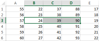
How to insert a cell in an Excel spreadsheet? Let’s say we have a table of values to which you want to insert two empty cells in between.
Perform the following procedure:
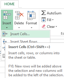
- Select the range in the place where you need to add new empty blocks. Go to the tab «HOME» — «Insert» — «Insert Cells». Or simply right click on the highlighted area and select the paste option. Or you may press the hotkey combination CTRL + SHIFT + «+».
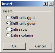
- A «Insert» dialog box appears where it is necessary to set the required parameters. In this case select «Shift down».
- Click OK. After that in the table with values new cells will be added. And the old will retain values and move down giving its place.
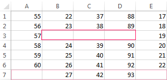
In this situation you can simply press the tool «HOME» — «Insert» (without choosing other options). Then the new cells will be inserted and the old ones will shift down (by default) without calling the dialog box options.
Use hotkeys combination CTRL + SHIFT + «plus» to add cells in Excel after selecting them.
Note. Pay attention to the settings dialog box. The last two parameters allow us to insert rows and columns in the same manner.
Removing cells
Now let’s remove the same range from our table with values. Just select the desired range. Right-click on the selected range and choose «Delete». Or go to the tab «HOME» — «Delete», «Shift up». The result is inversely proportional to the previous result.
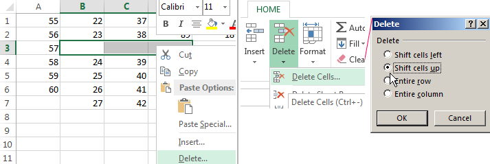
Select the range and use shortcut keys CTRL + «negative» if you want to remove cells in Excel.
Note. Likewise you can delete rows and columns.
Attention! In practice using tools «Insert» or «Delete» while inserting or deleting ranges without window with settings should be avoided so as not to get lost in the large and complex tables. Use the hotkeys if you want to save time. They cause a dialog box with removing the paste options and it also allows you to cope with the task much quickly.
In this Article
- Ranges and Cells in VBA
- Cell Address
- Range of Cells
- Writing to Cells
- Reading from Cells
- Non Contiguous Cells
- Intersection of Cells
- Offset from a Cell or Range
- Setting Reference to a Range
- Resize a Range
- OFFSET vs Resize
- All Cells in Sheet
- UsedRange
- CurrentRegion
- Range Properties
- Last Cell in Sheet
- Last Used Row Number in a Column
- Last Used Column Number in a Row
- Cell Properties
- Copy and Paste
- AutoFit Contents
- More Range Examples
- For Each
- Sort
- Find
- Range Address
- Range to Array
- Array to Range
- Sum Range
- Count Range
Ranges and Cells in VBA
Excel spreadsheets store data in Cells. Cells are arranged into Rows and Columns. Each cell can be identified by the intersection point of it’s row and column (Exs. B3 or R3C2).
An Excel Range refers to one or more cells (ex. A3:B4)
Cell Address
A1 Notation
In A1 notation, a cell is referred to by it’s column letter (from A to XFD) followed by it’s row number(from 1 to 1,048,576). This is called a cell address.
In VBA you can refer to any cell using the Range Object.
' Refer to cell B4 on the currently active sheet
MsgBox Range("B4")

' Refer to cell B4 on the sheet named 'Data'
MsgBox Worksheets("Data").Range("B4")

' Refer to cell B4 on the sheet named 'Data' in another OPEN workbook
' named 'My Data'
MsgBox Workbooks("My Data").Worksheets("Data").Range("B4")
R1C1 Notation
In R1C1 Notation a cell is referred by R followed by Row Number then letter ‘C’ followed by the Column Number. eg B4 in R1C1 notation will be referred by R4C2. In VBA you use the Cells Object to use R1C1 notation:
' Refer to cell R[6]C[4] i.e D6
Cells(6, 4) = "D6"
Range of Cells
A1 Notation
To refer to a more than one cell use a “:” between the starting cell address and last cell address. The following will refer to all the cells from A1 to D10:
Range("A1:D10")
R1C1 Notation
To refer to a more than one cell use a “,” between the starting cell address and last cell address. The following will refer to all the cells from A1 to D10:
Range(Cells(1, 1), Cells(10, 4))Writing to Cells
To write values to a cell or contiguous group of cells, simple refer to the range, put an = sign and then write the value to be stored:
' Store F5 in cell with Address F6
Range("F6") = "F6"

' Store E6 in cell with Address R[6]C[5] i.e E6
Cells(6, 5) = "E6"

' Store A1:D10 in the range A1:D10
Range("A1:D10") = "A1:D10"
' or
Range(Cells(1, 1), Cells(10, 4)) = "A1:D10"
Reading from Cells
To read values from cells, simple refer to the variable to store the values, put an = sign and then refer to the range to be read:
Dim val1
Dim val2

' Read from cell F6
val1 = Range("F6")

' Read from cell E6
val2 = Cells(6, 5)

MsgBox val1
Msgbox val2
Note: To store values from a range of cells, you need to use an Array instead of a simple variable.
Non Contiguous Cells
To refer to non contiguous cells use a comma between the cell addresses:
' Store 10 in cells A1, A3, and A5
Range("A1,A3,A5") = 10


' Store 10 in cells A1:A3 and D1:D3)
Range("A1:A3, D1:D3") = 10
VBA Coding Made Easy
Stop searching for VBA code online. Learn more about AutoMacro — A VBA Code Builder that allows beginners to code procedures from scratch with minimal coding knowledge and with many time-saving features for all users!

Learn More
Intersection of Cells
To refer to non contiguous cells use a space between the cell addresses:
' Store 'Col D' in D1:D10
' which is Common between A1:D10 and D1:F10
Range("A1:D10 D1:G10") = "Col D"
Offset from a Cell or Range
Using the Offset function, you can move the reference from a given Range (cell or group of cells) by the specified number_of_rows, and number_of_columns.
Offset Syntax
Range.Offset(number_of_rows, number_of_columns)
Offset from a cell
' OFFSET from a cell A1
' Refer to cell itself
' Move 0 rows and 0 columns
Range("A1").Offset(0, 0) = "A1"

' Move 1 rows and 0 columns
Range("A1").Offset(1, 0) = "A2"

' Move 0 rows and 1 columns
Range("A1").Offset(0, 1) = "B1"

' Move 1 rows and 1 columns
Range("A1").Offset(1, 1) = "B2"

' Move 10 rows and 5 columns
Range("A1").Offset(10, 5) = "F11"
Offset from a Range
' Move Reference to Range A1:D4 by 4 rows and 4 columns
' New Reference is E5:H8
Range("A1:D4").Offset(4,4) = "E5:H8"
Setting Reference to a Range
To assign a range to a range variable: declare a variable of type Range then use the Set command to set it to a range. Please note that you must use the SET command as RANGE is an object:
' Declare a Range variable
Dim myRange as Range

' Set the variable to the range A1:D4
Set myRange = Range("A1:D4")

' Prints $A$1:$D$4
MsgBox myRange.Address
VBA Programming | Code Generator does work for you!
Resize a Range
Resize method of Range object changes the dimension of the reference range:
Dim myRange As Range

' Range to Resize
Set myRange = Range("A1:F4")

' Prints $A$1:$E$10
Debug.Print myRange.Resize(10, 5).Address
Top-left cell of the Resized range is same as the top-left cell of the original range
Resize Syntax
Range.Resize(number_of_rows, number_of_columns)
OFFSET vs Resize
Offset does not change the dimensions of the range but moves it by the specified number of rows and columns. Resize does not change the position of the original range but changes the dimensions to the specified number of rows and columns.
All Cells in Sheet
The Cells object refers to all the cells in the sheet (1048576 rows and 16384 columns).
' Clear All Cells in Worksheets
Cells.Clear
UsedRange
UsedRange property gives you the rectangular range from the top-left cell used cell to the right-bottom used cell of the active sheet.
Dim ws As Worksheet
Set ws = ActiveSheet

' $B$2:$L$14 if L2 is the first cell with any value
' and L14 is the last cell with any value on the
' active sheet
Debug.Print ws.UsedRange.Address
CurrentRegion
CurrentRegion property gives you the contiguous rectangular range from the top-left cell to the right-bottom used cell containing the referenced cell/range.
Dim myRange As Range

Set myRange = Range("D4:F6")

' Prints $B$2:$L$14
' If there is a filled path from D4:F16 to B2 AND L14
Debug.Print myRange.CurrentRegion.Address

' You can refer to a single starting cell also

Set myRange = Range("D4") ' Prints $B$2:$L$14
AutoMacro | Ultimate VBA Add-in | Click for Free Trial!
Range Properties
You can get Address, row/column number of a cell, and number of rows/columns in a range as given below:
Dim myRange As Range

Set myRange = Range("A1:F10")

' Prints $A$1:$F$10
Debug.Print myRange.Address

Set myRange = Range("F10")

' Prints 10 for Row 10
Debug.Print myRange.Row

' Prints 6 for Column F
Debug.Print myRange.Column

Set myRange = Range("E1:F5")
' Prints 5 for number of Rows in range
Debug.Print myRange.Rows.Count

' Prints 2 for number of Columns in range
Debug.Print myRange.Columns.Count
Last Cell in Sheet
You can use Rows.Count and Columns.Count properties with Cells object to get the last cell on the sheet:
' Print the last row number
' Prints 1048576
Debug.Print "Rows in the sheet: " & Rows.Count

' Print the last column number
' Prints 16384
Debug.Print "Columns in the sheet: " & Columns.Count

' Print the address of the last cell
' Prints $XFD$1048576
Debug.Print "Address of Last Cell in the sheet: " & Cells(Rows.Count, Columns.Count)
Last Used Row Number in a Column
END property takes you the last cell in the range, and End(xlUp) takes you up to the first used cell from that cell.
Dim lastRow As Long

lastRow = Cells(Rows.Count, "A").End(xlUp).Row
Last Used Column Number in a Row
Dim lastCol As Long

lastCol = Cells(1, Columns.Count).End(xlToLeft).Column
END property takes you the last cell in the range, and End(xlToLeft) takes you left to the first used cell from that cell.
You can also use xlDown and xlToRight properties to navigate to the first bottom or right used cells of the current cell.
AutoMacro | Ultimate VBA Add-in | Click for Free Trial!
Cell Properties
Common Properties
Here is code to display commonly used Cell Properties
Dim cell As Range
Set cell = Range("A1")

cell.Activate
Debug.Print cell.Address
' Print $A$1

Debug.Print cell.Value
' Prints 456
' Address

Debug.Print cell.Formula
' Prints =SUM(C2:C3)

' Comment
Debug.Print cell.Comment.Text

' Style
Debug.Print cell.Style

' Cell Format
Debug.Print cell.DisplayFormat.NumberFormat
Cell Font
Cell.Font object contains properties of the Cell Font:
Dim cell As Range

Set cell = Range("A1")

' Regular, Italic, Bold, and Bold Italic
cell.Font.FontStyle = "Bold Italic"
' Same as
cell.Font.Bold = True
cell.Font.Italic = True

' Set font to Courier
cell.Font.FontStyle = "Courier"

' Set Font Color
cell.Font.Color = vbBlue
' or
cell.Font.Color = RGB(255, 0, 0)

' Set Font Size
cell.Font.Size = 20
Copy and Paste
Paste All
Ranges/Cells can be copied and pasted from one location to another. The following code copies all the properties of source range to destination range (equivalent to CTRL-C and CTRL-V)
'Simple Copy
Range("A1:D20").Copy
Worksheets("Sheet2").Range("B10").Paste

'or
' Copy from Current Sheet to sheet named 'Sheet2'
Range("A1:D20").Copy destination:=Worksheets("Sheet2").Range("B10")
Paste Special
Selected properties of the source range can be copied to the destination by using PASTESPECIAL option:
' Paste the range as Values only
Range("A1:D20").Copy
Worksheets("Sheet2").Range("B10").PasteSpecial Paste:=xlPasteValues
Here are the possible options for the Paste option:
' Paste Special Types
xlPasteAll
xlPasteAllExceptBorders
xlPasteAllMergingConditionalFormats
xlPasteAllUsingSourceTheme
xlPasteColumnWidths
xlPasteComments
xlPasteFormats
xlPasteFormulas
xlPasteFormulasAndNumberFormats
xlPasteValidation
xlPasteValues
xlPasteValuesAndNumberFormats
AutoFit Contents
Size of rows and columns can be changed to fit the contents using AutoFit:
' Change size of rows 1 to 5 to fit contents
Rows("1:5").AutoFit

' Change size of Columns A to B to fit contents
Columns("A:B").AutoFit
More Range Examples
It is recommended that you use Macro Recorder while performing the required action through the GUI. It will help you understand the various options available and how to use them.
AutoMacro | Ultimate VBA Add-in | Click for Free Trial!
For Each
It is easy to loop through a range using For Each construct as show below:
For Each cell In Range("A1:B100")
    ' Do something with the cell
Next cell
At each iteration of the loop one cell in the range is assigned to the variable cell and statements in the For loop are executed for that cell. Loop exits when all the cells are processed.
Sort
Sort is a method of Range object. You can sort a range by specifying options for sorting to Range.Sort. The code below will sort the columns A:C based on key in cell C2. Sort Order can be xlAscending or xlDescending. Header:= xlYes should be used if first row is the header row.
   Columns("A:C").Sort key1:=Range("C2"), _
      order1:=xlAscending, Header:=xlYes
Find
Find is also a method of Range Object. It find the first cell having content matching the search criteria and returns the cell as a Range object. It return Nothing if there is no match.
Use FindNext method (or FindPrevious) to find next(previous) occurrence.
Following code will change the font to “Arial Black” for all cells in the range which start with “John”:
For Each c In Range("A1:A100")
    If c Like "John*" Then
        c.Font.Name = "Arial Black"
    End If
Next c
Following code will replace all occurrences of “To Test” to “Passed” in the range specified:
With Range("a1:a500")
    Set c = .Find("To Test", LookIn:=xlValues)
    If Not c Is Nothing Then
        firstaddress = c.Address
        Do
            c.Value = "Passed"
            Set c = .FindNext(c)
        Loop While Not c Is Nothing And c.Address <> firstaddress
    End If
End With
It is important to note that you must specify a range to use FindNext. Also you must provide a stopping condition otherwise the loop will execute forever. Normally address of the first cell which is found is stored in a variable and loop is stopped when you reach that cell again. You must also check for the case when nothing is found to stop the loop.
Range Address
Use Range.Address to get the address in A1 Style
MsgBox Range("A1:D10").Address
' or
Debug.Print Range("A1:D10").Address
Use xlReferenceStyle (default is xlA1) to get addres in R1C1 style
MsgBox Range("A1:D10").Address(ReferenceStyle:=xlR1C1)
' or
Debug.Print Range("A1:D10").Address(ReferenceStyle:=xlR1C1)
This is useful when you deal with ranges stored in variables and want to process for certain addresses only.
AutoMacro | Ultimate VBA Add-in | Click for Free Trial!
Range to Array
It is faster and easier to transfer a range to an array and then process the values. You should declare the array as Variant to avoid calculating the size required to populate the range in the array. Array’s dimensions are set to match number of values in the range.
Dim DirArray As Variant
' Store the values in the range to the Array

DirArray = Range("a1:a5").Value

' Loop to process the values
For Each c In DirArray
    Debug.Print c
Next
Array to Range
After processing you can write the Array back to a Range. To write the Array in the example above to a Range you must specify a Range whose size matches the number of elements in the Array.
Use the code below to write the Array to the range D1:D5:
Range("D1:D5").Value = DirArray

Range("D1:H1").Value = Application.Transpose(DirArray)
Please note that you must Transpose the Array if you write it to a row.
Sum Range
SumOfRange = Application.WorksheetFunction.Sum(Range("A1:A10"))
Debug.Print SumOfRange
You can use many functions available in Excel in your VBA code by specifying Application.WorkSheetFunction. before the Function Name as in the example above.
Count Range
' Count Number of Cells with Numbers in the Range
CountOfCells = Application.WorksheetFunction.Count(Range("A1:A10"))
Debug.Print CountOfCells

' Count Number of Non Blank Cells in the Range
CountOfNonBlankCells = Application.WorksheetFunction.CountA(Range("A1:A10"))
Debug.Print CountOfNonBlankCells
Written by: Vinamra Chandra
“It is a capital mistake to theorize before one has data”- Sir Arthur Conan Doyle
This post covers everything you need to know about using Cells and Ranges in VBA. You can read it from start to finish as it is laid out in a logical order. If you prefer you can use the table of contents below to go to a section of your choice.
Topics covered include Offset property, reading values between cells, reading values to arrays and formatting cells.
A Quick Guide to Ranges and Cells
| Function | Takes | Returns | Example | Gives |
|---|---|---|---|---|
|
Range |
cell address | multiple cells | .Range(«A1:A4») | $A$1:$A$4 |
| Cells | row, column | one cell | .Cells(1,5) | $E$1 |
| Offset | row, column | multiple cells | Range(«A1:A2») .Offset(1,2) |
$C$2:$C$3 |
| Rows | row(s) | one or more rows | .Rows(4) .Rows(«2:4») |
$4:$4 $2:$4 |
| Columns | column(s) | one or more columns | .Columns(4) .Columns(«B:D») |
$D:$D $B:$D |
Download the Code
The Webinar
If you are a member of the VBA Vault, then click on the image below to access the webinar and the associated source code.
(Note: Website members have access to the full webinar archive.)

Introduction
This is the third post dealing with the three main elements of VBA. These three elements are the Workbooks, Worksheets and Ranges/Cells. Cells are by far the most important part of Excel. Almost everything you do in Excel starts and ends with Cells.
Generally speaking, you do three main things with Cells
- Read from a cell.
- Write to a cell.
- Change the format of a cell.
Excel has a number of methods for accessing cells such as Range, Cells and Offset.These can cause confusion as they do similar things and can lead to confusion
In this post I will tackle each one, explain why you need it and when you should use it.
Let’s start with the simplest method of accessing cells – using the Range property of the worksheet.
Important Notes
I have recently updated this article so that is uses Value2.
You may be wondering what is the difference between Value, Value2 and the default:
' Value2
Range("A1").Value2 = 56

' Value
Range("A1").Value = 56

' Default uses value
Range("A1") = 56
Using Value may truncate number if the cell is formatted as currency. If you don’t use any property then the default is Value.
It is better to use Value2 as it will always return the actual cell value(see this article from Charle Williams.)
The Range Property
The worksheet has a Range property which you can use to access cells in VBA. The Range property takes the same argument that most Excel Worksheet functions take e.g. “A1”, “A3:C6” etc.
The following example shows you how to place a value in a cell using the Range property.
' https://excelmacromastery.com/
Public Sub WriteToCell()

    ' Write number to cell A1 in sheet1 of this workbook
    ThisWorkbook.Worksheets("Sheet1").Range("A1").Value2 = 67

    ' Write text to cell A2 in sheet1 of this workbook
    ThisWorkbook.Worksheets("Sheet1").Range("A2").Value2 = "John Smith"

    ' Write date to cell A3 in sheet1 of this workbook
    ThisWorkbook.Worksheets("Sheet1").Range("A3").Value2 = #11/21/2017#

End Sub
As you can see Range is a member of the worksheet which in turn is a member of the Workbook. This follows the same hierarchy as in Excel so should be easy to understand. To do something with Range you must first specify the workbook and worksheet it belongs to.
For the rest of this post I will use the code name to reference the worksheet.

The following code shows the above example using the code name of the worksheet i.e. Sheet1 instead of ThisWorkbook.Worksheets(“Sheet1”).
' https://excelmacromastery.com/
Public Sub UsingCodeName()

    ' Write number to cell A1 in sheet1 of this workbook
    Sheet1.Range("A1").Value2 = 67

    ' Write text to cell A2 in sheet1 of this workbook
    Sheet1.Range("A2").Value2 = "John Smith"

    ' Write date to cell A3 in sheet1 of this workbook
    Sheet1.Range("A3").Value2 = #11/21/2017#

End Sub
You can also write to multiple cells using the Range property
' https://excelmacromastery.com/
Public Sub WriteToMulti()

    ' Write number to a range of cells
    Sheet1.Range("A1:A10").Value2 = 67

    ' Write text to multiple ranges of cells
    Sheet1.Range("B2:B5,B7:B9").Value2 = "John Smith"

End Sub
You can download working examples of all the code from this post from the top of this article.
The Cells Property of the Worksheet
The worksheet object has another property called Cells which is very similar to range. There are two differences
- Cells returns a range of one cell only.
- Cells takes row and column as arguments.
The example below shows you how to write values to cells using both the Range and Cells property
' https://excelmacromastery.com/
Public Sub UsingCells()

    ' Write to A1
    Sheet1.Range("A1").Value2 = 10
    Sheet1.Cells(1, 1).Value2  = 10

    ' Write to A10
    Sheet1.Range("A10").Value2 = 10
    Sheet1.Cells(10, 1).Value2  = 10

    ' Write to E1
    Sheet1.Range("E1").Value2 = 10
    Sheet1.Cells(1, 5).Value2  = 10

End Sub
You may be wondering when you should use Cells and when you should use Range. Using Range is useful for accessing the same cells each time the Macro runs.
For example, if you were using a Macro to calculate a total and write it to cell A10 every time then Range would be suitable for this task.
Using the Cells property is useful if you are accessing a cell based on a number that may vary. It is easier to explain this with an example.
In the following code, we ask the user to specify the column number. Using Cells gives us the flexibility to use a variable number for the column.
' https://excelmacromastery.com/
Public Sub WriteToColumn()

    Dim UserCol As Integer

    ' Get the column number from the user
    UserCol = Application.InputBox(" Please enter the column...", Type:=1)

    ' Write text to user selected column
    Sheet1.Cells(1, UserCol).Value2 = "John Smith"

End Sub
In the above example, we are using a number for the column rather than a letter.
To use Range here would require us to convert these values to the letter/number cell reference e.g. “C1”. Using the Cells property allows us to provide a row and a column number to access a cell.
Sometimes you may want to return more than one cell using row and column numbers. The next section shows you how to do this.
Using Cells and Range together
As you have seen you can only access one cell using the Cells property. If you want to return a range of cells then you can use Cells with Ranges as follows
' https://excelmacromastery.com/
Public Sub UsingCellsWithRange()

    With Sheet1
        ' Write 5 to Range A1:A10 using Cells property
        .Range(.Cells(1, 1), .Cells(10, 1)).Value2 = 5

        ' Format Range B1:Z1 to be bold
        .Range(.Cells(1, 2), .Cells(1, 26)).Font.Bold = True

    End With

End Sub
As you can see, you provide the start and end cell of the Range. Sometimes it can be tricky to see which range you are dealing with when the value are all numbers. Range has a property called Address which displays the letter/ number cell reference of any range. This can come in very handy when you are debugging or writing code for the first time.
In the following example we print out the address of the ranges we are using:
' https://excelmacromastery.com/
Public Sub ShowRangeAddress()

    ' Note: Using underscore allows you to split up lines of code
    With Sheet1

        ' Write 5 to Range A1:A10 using Cells property
        .Range(.Cells(1, 1), .Cells(10, 1)).Value2 = 5
        Debug.Print "First address is : " _
            + .Range(.Cells(1, 1), .Cells(10, 1)).Address

        ' Format Range B1:Z1 to be bold
        .Range(.Cells(1, 2), .Cells(1, 26)).Font.Bold = True
        Debug.Print "Second address is : " _
            + .Range(.Cells(1, 2), .Cells(1, 26)).Address

    End With

End Sub
In the example I used Debug.Print to print to the Immediate Window. To view this window select View->Immediate Window(or Ctrl G)


You can download all the code for this post from the top of this article.
The Offset Property of Range
Range has a property called Offset. The term Offset refers to a count from the original position. It is used a lot in certain areas of programming. With the Offset property you can get a Range of cells the same size and a certain distance from the current range. The reason this is useful is that sometimes you may want to select a Range based on a certain condition. For example in the screenshot below there is a column for each day of the week. Given the day number(i.e. Monday=1, Tuesday=2 etc.) we need to write the value to the correct column.

We will first attempt to do this without using Offset.
' https://excelmacromastery.com/
' This sub tests with different values
Public Sub TestSelect()

    ' Monday
    SetValueSelect 1, 111.21
    ' Wednesday
    SetValueSelect 3, 456.99
    ' Friday
    SetValueSelect 5, 432.25
    ' Sunday
    SetValueSelect 7, 710.17

End Sub

' Writes the value to a column based on the day
Public Sub SetValueSelect(lDay As Long, lValue As Currency)

    Select Case lDay
        Case 1: Sheet1.Range("H3").Value2 = lValue
        Case 2: Sheet1.Range("I3").Value2 = lValue
        Case 3: Sheet1.Range("J3").Value2 = lValue
        Case 4: Sheet1.Range("K3").Value2 = lValue
        Case 5: Sheet1.Range("L3").Value2 = lValue
        Case 6: Sheet1.Range("M3").Value2 = lValue
        Case 7: Sheet1.Range("N3").Value2 = lValue
    End Select

End Sub
As you can see in the example, we need to add a line for each possible option. This is not an ideal situation. Using the Offset Property provides a much cleaner solution
' https://excelmacromastery.com/
' This sub tests with different values
Public Sub TestOffset()

    DayOffSet 1, 111.01
    DayOffSet 3, 456.99
    DayOffSet 5, 432.25
    DayOffSet 7, 710.17

End Sub

Public Sub DayOffSet(lDay As Long, lValue As Currency)

    ' We use the day value with offset specify the correct column
    Sheet1.Range("G3").Offset(, lDay).Value2 = lValue

End Sub
As you can see this solution is much better. If the number of days in increased then we do not need to add any more code. For Offset to be useful there needs to be some kind of relationship between the positions of the cells. If the Day columns in the above example were random then we could not use Offset. We would have to use the first solution.
One thing to keep in mind is that Offset retains the size of the range. So .Range(“A1:A3”).Offset(1,1) returns the range B2:B4. Below are some more examples of using Offset
' https://excelmacromastery.com/
Public Sub UsingOffset()

    ' Write to B2 - no offset
    Sheet1.Range("B2").Offset().Value2 = "Cell B2"

    ' Write to C2 - 1 column to the right
    Sheet1.Range("B2").Offset(, 1).Value2 = "Cell C2"

    ' Write to B3 - 1 row down
    Sheet1.Range("B2").Offset(1).Value2 = "Cell B3"

    ' Write to C3 - 1 column right and 1 row down
    Sheet1.Range("B2").Offset(1, 1).Value2 = "Cell C3"

    ' Write to A1 - 1 column left and 1 row up
    Sheet1.Range("B2").Offset(-1, -1).Value2 = "Cell A1"

    ' Write to range E3:G13 - 1 column right and 1 row down
    Sheet1.Range("D2:F12").Offset(1, 1).Value2 = "Cells E3:G13"

End Sub
Using the Range CurrentRegion
CurrentRegion returns a range of all the adjacent cells to the given range.
In the screenshot below you can see the two current regions. I have added borders to make the current regions clear.

A row or column of blank cells signifies the end of a current region.
You can manually check the CurrentRegion in Excel by selecting a range and pressing Ctrl + Shift + *.
If we take any range of cells within the border and apply CurrentRegion, we will get back the range of cells in the entire area.
For example
Range(“B3”).CurrentRegion will return the range B3:D14
Range(“D14”).CurrentRegion will return the range B3:D14
Range(“C8:C9”).CurrentRegion will return the range B3:D14
and so on
How to Use
We get the CurrentRegion as follows
' Current region will return B3:D14 from above example
Dim rg As Range
Set rg = Sheet1.Range("B3").CurrentRegion
Read Data Rows Only
Read through the range from the second row i.e.skipping the header row
' Current region will return B3:D14 from above example
Dim rg As Range
Set rg = Sheet1.Range("B3").CurrentRegion

' Start at row 2 - row after header
Dim i As Long
For i = 2 To rg.Rows.Count
    ' current row, column 1 of range
    Debug.Print rg.Cells(i, 1).Value2
Next i
Remove Header
Remove header row(i.e. first row) from the range. For example if range is A1:D4 this will return A2:D4
' Current region will return B3:D14 from above example
Dim rg As Range
Set rg = Sheet1.Range("B3").CurrentRegion

' Remove Header
Set rg = rg.Resize(rg.Rows.Count - 1).Offset(1)

' Start at row 1 as no header row
Dim i As Long
For i = 1 To rg.Rows.Count
    ' current row, column 1 of range
    Debug.Print rg.Cells(i, 1).Value2
Next i
Using Rows and Columns as Ranges
If you want to do something with an entire Row or Column you can use the Rows or Columns property of the Worksheet. They both take one parameter which is the row or column number you wish to access
' https://excelmacromastery.com/
Public Sub UseRowAndColumns()

    ' Set the font size of column B to 9
    Sheet1.Columns(2).Font.Size = 9

    ' Set the width of columns D to F
    Sheet1.Columns("D:F").ColumnWidth = 4

    ' Set the font size of row 5 to 18
    Sheet1.Rows(5).Font.Size = 18

End Sub
Using Range in place of Worksheet
You can also use Cells, Rows and Columns as part of a Range rather than part of a Worksheet. You may have a specific need to do this but otherwise I would avoid the practice. It makes the code more complex. Simple code is your friend. It reduces the possibility of errors.
The code below will set the second column of the range to bold. As the range has only two rows the entire column is considered B1:B2
' https://excelmacromastery.com/
Public Sub UseColumnsInRange()

    ' This will set B1 and B2 to be bold
    Sheet1.Range("A1:C2").Columns(2).Font.Bold = True

End Sub
You can download all the code for this post from the top of this article.
Reading Values from one Cell to another
In most of the examples so far we have written values to a cell. We do this by placing the range on the left of the equals sign and the value to place in the cell on the right. To write data from one cell to another we do the same. The destination range goes on the left and the source range goes on the right.
The following example shows you how to do this:
' https://excelmacromastery.com/
Public Sub ReadValues()

    ' Place value from B1 in A1
    Sheet1.Range("A1").Value2 = Sheet1.Range("B1").Value2

    ' Place value from B3 in sheet2 to cell A1
    Sheet1.Range("A1").Value2 = Sheet2.Range("B3").Value2

    ' Place value from B1 in cells A1 to A5
    Sheet1.Range("A1:A5").Value2 = Sheet1.Range("B1").Value2

    ' You need to use the "Value" property to read multiple cells
    Sheet1.Range("A1:A5").Value2 = Sheet1.Range("B1:B5").Value2

End Sub
As you can see from this example it is not possible to read from multiple cells. If you want to do this you can use the Copy function of Range with the Destination parameter
' https://excelmacromastery.com/
Public Sub CopyValues()

    ' Store the copy range in a variable
    Dim rgCopy As Range
    Set rgCopy = Sheet1.Range("B1:B5")

    ' Use this to copy from more than one cell
    rgCopy.Copy Destination:=Sheet1.Range("A1:A5")

    ' You can paste to multiple destinations
    rgCopy.Copy Destination:=Sheet1.Range("A1:A5,C2:C6")

End Sub
The Copy function copies everything including the format of the cells. It is the same result as manually copying and pasting a selection. You can see more about it in the Copying and Pasting Cells section.
Using the Range.Resize Method
When copying from one range to another using assignment(i.e. the equals sign), the destination range must be the same size as the source range.
Using the Resize function allows us to resize a range to a given number of rows and columns.
For example:
' https://excelmacromastery.com/
Sub ResizeExamples()

    ' Prints A1
    Debug.Print Sheet1.Range("A1").Address

    ' Prints A1:A2
    Debug.Print Sheet1.Range("A1").Resize(2, 1).Address

    ' Prints A1:A5
    Debug.Print Sheet1.Range("A1").Resize(5, 1).Address

    ' Prints A1:D1
    Debug.Print Sheet1.Range("A1").Resize(1, 4).Address

    ' Prints A1:C3
    Debug.Print Sheet1.Range("A1").Resize(3, 3).Address

End Sub
When we want to resize our destination range we can simply use the source range size.
In other words, we use the row and column count of the source range as the parameters for resizing:
' https://excelmacromastery.com/
Sub Resize()

    Dim rgSrc As Range, rgDest As Range

    ' Get all the data in the current region
    Set rgSrc = Sheet1.Range("A1").CurrentRegion

      ' Get the range destination
    Set rgDest = Sheet2.Range("A1")
    Set rgDest = rgDest.Resize(rgSrc.Rows.Count, rgSrc.Columns.Count)

    rgDest.Value2 = rgSrc.Value2

End Sub
We can do the resize in one line if we prefer:
' https://excelmacromastery.com/
Sub ResizeOneLine()

    Dim rgSrc As Range

    ' Get all the data in the current region
    Set rgSrc = Sheet1.Range("A1").CurrentRegion

    With rgSrc
        Sheet2.Range("A1").Resize(.Rows.Count, .Columns.Count).Value2 = .Value2
    End With

End Sub
Reading Values to variables
We looked at how to read from one cell to another. You can also read from a cell to a variable. A variable is used to store values while a Macro is running. You normally do this when you want to manipulate the data before writing it somewhere. The following is a simple example using a variable. As you can see the value of the item to the right of the equals is written to the item to the left of the equals.
' https://excelmacromastery.com/
Public Sub UseVariables()

    ' Create
    Dim number As Long

    ' Read number from cell
    number = Sheet1.Range("A1").Value2

    ' Add 1 to value
    number = number + 1

    ' Write new value to cell
    Sheet1.Range("A2").Value2 = number

End Sub
To read text to a variable you use a variable of type String:
' https://excelmacromastery.com/
Public Sub UseVariableText()

    ' Declare a variable of type string
    Dim text As String

    ' Read value from cell
    text = Sheet1.Range("A1").Value2

    ' Write value to cell
    Sheet1.Range("A2").Value2 = text

End Sub
You can write a variable to a range of cells. You just specify the range on the left and the value will be written to all cells in the range.
' https://excelmacromastery.com/
Public Sub VarToMulti()

    ' Read value from cell
    Sheet1.Range("A1:B10").Value2 = 66

End Sub
You cannot read from multiple cells to a variable. However you can read to an array which is a collection of variables. We will look at doing this in the next section.
How to Copy and Paste Cells
If you want to copy and paste a range of cells then you do not need to select them. This is a common error made by new VBA users.
Note: We normally use Range.Copy when we want to copy formats, formulas, validation. If we want to copy values it is not the most efficient method.
I have written a complete guide to copying data in Excel VBA here.
You can simply copy a range of cells like this:
Range("A1:B4").Copy Destination:=Range("C5")
Using this method copies everything – values, formats, formulas and so on. If you want to copy individual items you can use the PasteSpecial property of range.
It works like this
Range("A1:B4").Copy
Range("F3").PasteSpecial Paste:=xlPasteValues
Range("F3").PasteSpecial Paste:=xlPasteFormats
Range("F3").PasteSpecial Paste:=xlPasteFormulas
The following table shows a full list of all the paste types
| Paste Type |
|---|
| xlPasteAll |
| xlPasteAllExceptBorders |
| xlPasteAllMergingConditionalFormats |
| xlPasteAllUsingSourceTheme |
| xlPasteColumnWidths |
| xlPasteComments |
| xlPasteFormats |
| xlPasteFormulas |
| xlPasteFormulasAndNumberFormats |
| xlPasteValidation |
| xlPasteValues |
| xlPasteValuesAndNumberFormats |
Reading a Range of Cells to an Array
You can also copy values by assigning the value of one range to another.
Range("A3:Z3").Value2 = Range("A1:Z1").Value2
The value of range in this example is considered to be a variant array. What this means is that you can easily read from a range of cells to an array. You can also write from an array to a range of cells. If you are not familiar with arrays you can check them out in this post.
The following code shows an example of using an array with a range:
' https://excelmacromastery.com/
Public Sub ReadToArray()

    ' Create dynamic array
    Dim StudentMarks() As Variant

    ' Read 26 values into array from the first row
    StudentMarks = Range("A1:Z1").Value2

    ' Do something with array here

    ' Write the 26 values to the third row
    Range("A3:Z3").Value2 = StudentMarks

End Sub
Keep in mind that the array created by the read is a 2 dimensional array. This is because a spreadsheet stores values in two dimensions i.e. rows and columns
Going through all the cells in a Range
Sometimes you may want to go through each cell one at a time to check value.
You can do this using a For Each loop shown in the following code
' https://excelmacromastery.com/
Public Sub TraversingCells()

    ' Go through each cells in the range
    Dim rg As Range
    For Each rg In Sheet1.Range("A1:A10,A20")
        ' Print address of cells that are negative
        If rg.Value < 0 Then
            Debug.Print rg.Address + " is negative."
        End If
    Next

End Sub
You can also go through consecutive Cells using the Cells property and a standard For loop.
The standard loop is more flexible about the order you use but it is slower than a For Each loop.
' https://excelmacromastery.com/
Public Sub TraverseCells()

    ' Go through cells from A1 to A10
    Dim i As Long
    For i = 1 To 10
        ' Print address of cells that are negative
        If Range("A" & i).Value < 0 Then
            Debug.Print Range("A" & i).Address + " is negative."
        End If
    Next

    ' Go through cells in reverse i.e. from A10 to A1
    For i = 10 To 1 Step -1
        ' Print address of cells that are negative
        If Range("A" & i) < 0 Then
            Debug.Print Range("A" & i).Address + " is negative."
        End If
    Next

End Sub
Formatting Cells
Sometimes you will need to format the cells the in spreadsheet. This is actually very straightforward. The following example shows you various formatting you can add to any range of cells
' https://excelmacromastery.com/
Public Sub FormattingCells()

    With Sheet1

        ' Format the font
        .Range("A1").Font.Bold = True
        .Range("A1").Font.Underline = True
        .Range("A1").Font.Color = rgbNavy

        ' Set the number format to 2 decimal places
        .Range("B2").NumberFormat = "0.00"
        ' Set the number format to a date
        .Range("C2").NumberFormat = "dd/mm/yyyy"
        ' Set the number format to general
        .Range("C3").NumberFormat = "General"
        ' Set the number format to text
        .Range("C4").NumberFormat = "Text"

        ' Set the fill color of the cell
        .Range("B3").Interior.Color = rgbSandyBrown

        ' Format the borders
        .Range("B4").Borders.LineStyle = xlDash
        .Range("B4").Borders.Color = rgbBlueViolet

    End With

End Sub
Main Points
The following is a summary of the main points
- Range returns a range of cells
- Cells returns one cells only
- You can read from one cell to another
- You can read from a range of cells to another range of cells.
- You can read values from cells to variables and vice versa.
- You can read values from ranges to arrays and vice versa
- You can use a For Each or For loop to run through every cell in a range.
- The properties Rows and Columns allow you to access a range of cells of these types
What’s Next?
Free VBA Tutorial If you are new to VBA or you want to sharpen your existing VBA skills then why not try out the The Ultimate VBA Tutorial.
Related Training: Get full access to the Excel VBA training webinars and all the tutorials.
(NOTE: Planning to build or manage a VBA Application? Learn how to build 10 Excel VBA applications from scratch.)
Cell, Row, Column | Range Examples | Fill a Range | Move a Range | Copy/Paste a Range | Insert Row, Column
A range in Excel is a collection of two or more cells. This chapter gives an overview of some very important range operations.
Cell, Row, Column
Let’s start by selecting a cell, row and column.
1. To select cell C3, click on the box at the intersection of column C and row 3.

2. To select column C, click on the column C header.

3. To select row 3, click on the row 3 header.

Range Examples
A range is a collection of two or more cells.
1. To select the range B2:C4, click on cell B2 and drag it to cell C4.

2. To select a range of individual cells, hold down CTRL and click on each cell that you want to include in the range.

Fill a Range
To fill a range, execute the following steps.
1a. Enter the value 2 into cell B2.

1b. Select cell B2, click on the lower right corner of cell B2 and drag it down to cell B8.

Result:

This dragging technique is very important and you will use it very often in Excel. Here’s another example.
2a. Enter the value 2 into cell B2 and the value 4 into cell B3.

2b. Select cell B2 and cell B3, click on the lower right corner of this range and drag it down.

Excel automatically fills the range based on the pattern of the first two values. That’s pretty cool huh!? Here’s another example.
3a. Enter the date 6/13/2016 into cell B2 and the date 6/16/2016 into cell B3.

3b. Select cell B2 and cell B3, click on the lower right corner of this range and drag it down.

Note: visit our page about AutoFill for many more examples.
Move a Range
To move a range, execute the following steps.
1. Select a range and click on the border of the range.

2. Drag the range to its new location.

Copy/Paste a Range
To copy and paste a range, execute the following steps.
1. Select the range, right click, and then click Copy (or press CTRL + c).

2. Select the cell where you want the first cell of the range to appear, right click, and then click Paste under ‘Paste Options:’ (or press CTRL + v).

Insert Row, Column
To insert a row between the values 20 and 40 below, execute the following steps.
1. Select row 3.

2. Right click, and then click Insert.

Result.

The rows below the new row are shifted down. In a similar way, you can insert a column.
A Powerful & Multi-purpose Templates for project management. Now seamlessly manage your projects, tasks, meetings, presentations, teams, customers, stakeholders and time. This page describes all the amazing new features and options that come with our premium templates.
Save Up to 85% LIMITED TIME OFFER

All-in-One Pack
120+ Project Management Templates
Essential Pack
50+ Project Management Templates
Excel Pack
50+ Excel PM Templates
PowerPoint Pack
50+ Excel PM Templates
MS Word Pack
25+ Word PM Templates
Ultimate Project Management Template
Ultimate Resource Management Template
Project Portfolio Management Templates
- VBA Insert Cell or Range in a worksheet – Syntax
- VBA Insert Range in a Worksheet – xlDown
- VBA Insert Range in a Worksheet – xlToRight
- VBA Insert Range in a Worksheet – EntireRow
- VBA Insert Range in a Worksheet – EntireColumn
- VBA Insert Range in a Worksheet – Instructions
Page load link
Go to Top
Introduction to Range and Cells in VBA
When you look around in an Excel workbook, you will find that everything works around cells. A cell and a range of cells are where you store your data, and then everything starts.
To make the best of VBA, you need to learn how to use cells and ranges in your codes. For this, you need to have a solid understanding of Range objects. By using it, you can refer to cells in your codes in the following ways:
- A single cell.
- A range of cells
- A row or a column
- A three-dimensional range
The RANGE OBJECT is a part of Excel’s Object Hierarchy: Application ➜ Workbooks ➜ Worksheets ➜ Range and besides inside the worksheet. So if you are writing code to refer to the RANGE object it would be like this:
Application.Workbook(“Workbook-Name”).Worksheets(“Sheet-Name”).RangeBy referring to a cell or range of cells, you can do the following things:
- You can read the value from it.
- You can enter a value in it.
- And, you can make changes to the format.
To do all these things, you need to learn to refer to a cell or a range of cells, and in the next section of this tutorial, you will learn to refer to a cell using different ways.
To refer to a cell or a range of cells, you can use three different ways.
- Range Property
- Cells Property
- Offset Property
Well, which one is best out of these depends on your requirement, but it is worth learning all three so that you can choose which one is perfect for you.
So let’s get started.
Range Property
Range property is the most common and popular way to refer to a range in your VBA codes. With Range property, you simply need to refer to the cell address. Let me tell you the syntax.
expression.range(address)Here the expression is a variable representing a VBA object. So if you need to refer to the cell A1, the line of code you need to write would be:
Application.Workbook(“Book1”).Worksheets(“Sheet1”).Range(“A1”)The above code tells VBA that you are referring to cell A1 which is in the worksheet “Sheet1” and workbook ”Book1”.
Note: Whenever you type a cell address in the range object, make sure to wrap it in double quotation marks. But here’s one thing to understand. As you are using VBA in Excel there’s no need to use the word “Application”. So the code would be:
Workbook(“Book1”).Worksheets(“Sheet1”).Range(“A1”)And if you are in the Book1 there you can further trim down your code:
Worksheets(“Sheet1”).Range(“A1”)But, if you are already in the worksheet “Sheet1” then you can further trim down your code and can only use:
Range(“A1”)Now, let’s say if you want to refer to a full range of cells (i.e., multiple cells) you need to write the code in the following way:
Range("A1:A5")In the above code, you have referred to the range A1 to A5 which consists of the five cells. You can also refer to a named range using the range object. Let’s say you have named range with the name of “Sales Discount” to refer to this you can write a code like this:
Range("Sales Discount")If you want to refer to a non-continues range then you need to do something like this:
Range("A1:B5,D5:G10")And if you want to refer to an entire row or a column then you need to enter code like the below:
Range("1:1")
Range("A:A")
At this point, you have a clear understanding of how to refer to a cell and the range of cells. But to make it best with this you need to learn how to use this to do other things.
here we have a complete list of tutorials that you can use to learn to work with ranges and cells in VBA
- How to SET (Get and Change) Cell Value using a VBA Code
- How to Select a Range using VBA in Excel
- How to Create a Named Range using VBA (Static + Dynamic) in Excel
- How to Merge and Unmerge Cells in Excel using a VBA Code
- How to Check IF a Cell is Empty using VBA in Excel
- VBA ClearContents (from a Cell, Range, or Entire Worksheet)
- Excel VBA Font (Color, Size, Type, and Bold)
- How to AutoFit (Rows, Column, or the Entire Worksheet) using VBA
- How to use OFFSET Property with the Range Object or a Cell in VBA
- VBA Wrap Text (Cell, Range, and Entire Worksheet)
- How to Copy a CellRange to Another Sheet using VBA
- How to use Range/Cell as a Variable in VBA in Excel
- How to Find Last Rows, Column, and Cell using VBA in Excel
- How to use ActiveCell in VBA in Excel
- How to Refer to the UsedRange using VBA in Excel
- How to Change Row Height/Column Width using VBA in Excel
- How to SELECT ALL the Cells in a Worksheet using a VBA Code
- How to Insert a Row using VBA in Excel
- How to Insert a Column using VBA in Excel
1. Select and Activate a Cell
If you want to select a cell then you can use the Range. Select method. Let’s say if you want to select cell A5 then all you need to do is specify the range and then add “.Select” after that.
Range(“A1”).SelectThis code tells VBA to select cell A5 and if you want to select a range of cells then you just need to refer to that range and simply add “.Select” after that.
Range(“A1:A5”).SelectThere’s also another method that you can use to activate a cell.
Range(“A1”).ActivateHere you need to remember that you can activate only one cell at a time. Even if you specify a range with the “.Activate” method, it will select that range but the active cell will be the first cell of the range.
2. Enter a Value in a Cell
By using the range property you can enter a value in a cell or a range of cells. Let’s understand how it works using a simple example:
Range("A1").Value = "ExcelChamps"In the above example, you have specified the A1 as a range and after that, you have added “.Value” which tells VBA to access the value property of the cell.
The next thing you have is the equals sign and then the value which you want to enter (you need to use double quotation marks if you are entering a text value). For a number, the code would like this:
Range("A1").Value = 9988And if you want to enter a value into a range of cells, I mean multiple cells, then all you need to do is specify that range.
Range("A1:A5").Value = "ExcelChamps"And, here’s the code if you are referring to the non-continues range.
Range("A1:A5 , E2:E3").Value = "ExcelChamps"3. Copy and Paste a Cell/Range
With Range property, you can use the “.Copy” method to copy and cell and then paste it into a destination cell. Let’s say if you need to copy the cell A5 the code for this would be:
Range("A5").Copy When you run this code it will simply copy cell A5 but the next thing is to paste this copied cell to a destination cell. For this, you need to add the keyword destination after it and followed by the cell where you want to paste it. So if you want to copy cell A1 and then want to paste it to the cell E5, the code would be:
Range("A1").Copy Destination:=Range("E5")In the same way, if you are dealing with a range of multiple cells then the code would be like:
Range("A1:A5").Copy Destination:=Range("E5:E9")If you have copied a range of cells and then if you have mentioned one cell as the destination range, VBA will copy the entire copied range the starting from the cell you have specified as a destination.
Range("A1:A5").Copy Destination:=Range("B1")When you run the above code, VBA will copy range A1:A5 and will paste it to the B1:B5 even though you have mentioned only B1 as the destination range.
Tip: Just like the “.Copy” method you can use the “.Cut” method to cut a cell and then simply use a destination to paste it.
4. Use Font Property with Range Property
With the range property, you can access the font property of a cell which helps you to change all the font settings. There are a total of 18 different properties for the font which you can access. Let’s say if you want to make the text BOLD in cell A1, the code would be:
Range("A1").Font.Bold = TrueThis code tells VBA to access the BOLD property of the font which is inside the range A1 and you have set this property to TRUE. Now, let’s say you want to apply strikethrough to cell A1, this time the code would be:
As I said there are a total of 18 different properties you can use, so make sure to check out all of these to see which one is useful for you.
5. Clear Formatting from a Cell
By using the “.ClearFormats” method you can remove only the format from a cell or a range of cells. All you need to do is add “.ClearFormat” after specifying the range, like below:
Range("A1").ClearFormatsWhen you run the code above it clears all the formatting from cell A1 and if you want to do it for an entire range, you know what to do, Right?
Range("A1:A5").ClearFormatsNow the above code will simply remove the formatting from the range A1 to A5.
Cells Property
Apart from the RANGE property, you can use the “Cells” property to refer to a cell or a range of cells in your worksheet. In cell property, instead of using the cell reference, you need to enter the column number and row number of the cell.
expression.Cells(Row_Number, Column_Number)Here the expression is a VBA object and Row_Number is the row number of the cell and Column_Number is the column of the cell. So if you want to refer to the cell A5 you can use the code below code:
Cells(5,1)Now, this code tells VBA to refer to the cell which is at row number five and at column number one. As its syntax says you need to enter column number as address but the reality is you can also use the column alphabet if you want just by wrapping it in double quotation marks.
The below code will also refer to the cell A5:
Cells(5,"A")And to VBA to select it simply add “.Select” at the end.
Cells(5,1).SelectThe above code will select cell A5 which is in the 5th row and in the first column of the worksheet.
OFFSET Property
If you want to play well with ranges in VBA you need to know how to use the OFFSET property. It helps to refer to a cell that is a particular number of rows and columns away from another cell.
Let’s say your active cell is B5 right now and you want to navigate to the cell which is 3 columns right and 1 row down from B5, you can do this OFFSET. Below is the syntax which you need to use for the OFFSET:
expression.Offset (RowOffset, ColumnOffset)- RowOffset: In this argument, you need to specify a number that will tell VBA how many rows you want to navigate. A positive number defines a row downward and a negative number defines a row upward.
- ColumnOffset: In this argument, you need to specify a number that will tell VBA how many columns you want to navigate. A positive number defines a column to the right and a negative number defines a left.
Let’s write a simple code for example which we have discussed above.
- First, you need to define the range from where you want to navigate and so type the below code:

- After that, type “.Offset” and enter opening parentheses, just like below:

- Next, you need to enter the row number and then the column number where you want to navigate.

- In the end, you need to add “.Select” to tell VBA to select the cell where you want to navigate.


So when you run this code it will select the cell which is one row down and 3 columns right from cell B5.
Resize a Range using OFFSET
OFFSET not only allows you to navigate to a cell, but you can also resize the range further. Let’s continue the above example.
Range("B5").Offset(1, 3).SelectThe above code navigates you to cell E6, and now let’s say you need to select the range of cells that consists of the five columns and three rows from the E6. So what you need to do is after using OFFSET, use the resize property by adding “.Resize”.
Range("B5").Offset(1, 3).ResizeNow you need to enter the row size and column size. Type a starting parenthesis and enter the number to define the row size and then a number to define the column size.
Range("B5").Offset(1, 3).Resize(3,5)In the end, add “.Select” to tell VBA to select the range, and when you run this code, it will select the range.
Range("B5").Offset(1, 3).Resize(3, 5).SelectSo, when you run this code, it will select the range E6 to I8.
Range("A1").Font.Strikethrough = TrueMore Tutorials
- Count Rows using VBA in Excel
- Excel VBA Font (Color, Size, Type, and Bold)
- Excel VBA Hide and Unhide a Column or a Row
- Apply Borders on a Cell using VBA in Excel
- Find Last Row, Column, and Cell using VBA in Excel
- Insert a Row using VBA in Excel
- Merge Cells in Excel using a VBA Code
- Select a Range/Cell using VBA in Excel
- SELECT ALL the Cells in a Worksheet using a VBA Code
- ActiveCell in VBA in Excel
- Special Cells Method in VBA in Excel
- UsedRange Property in VBA in Excel
- VBA AutoFit (Rows, Column, or the Entire Worksheet)
- VBA ClearContents (from a Cell, Range, or Entire Worksheet)
- VBA Copy Range to Another Sheet + Workbook
- VBA Enter Value in a Cell (Set, Get and Change)
- VBA Insert Column (Single and Multiple)
- VBA Named Range | (Static + from Selection + Dynamic)
- VBA Range Offset
- VBA Sort Range | (Descending, Multiple Columns, Sort Orientation
- VBA Wrap Text (Cell, Range, and Entire Worksheet)
- VBA Check IF a Cell is Empty + Multiple Cells
⇠ Back to What is VBA in Excel
Helpful Links – Developer Tab – Visual Basic Editor – Run a Macro – Personal Macro Workbook – Excel Macro Recorder – VBA Interview Questions – VBA Codes