Add number to excel column - Word и Excel - помощь в работе с программами

Содержание

Add a list of numbers in a column
Ways to add values in a spreadsheet
Add based on conditions
Add or subtract dates
Add or subtract time
Need more help?
Add and subtract numbers
Add two or more numbers in one cell
Add numbers using cell references
Get a quick total from a row or column
Subtract two or more numbers in a cell
Subtract numbers using cell references
Add two or more numbers in one cell
Add numbers using cell references
Get a quick total from a row or column
Subtract two or more numbers in a cell
Subtract numbers using cell references
Automatically number rows
What do you want to do?
Fill a column with a series of numbers
Use the ROW function to number rows
Display or hide the fill handle
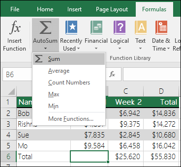
Use AutoSum to sum numbers
On your Android tablet or Android phone
Need more help?

Add a list of numbers in a column

To quickly get a total instead of typing each number into a calculator.

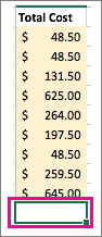
Click the first empty cell below a column of numbers.

Do one of the following:

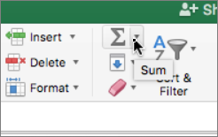
Excel 2016 for Mac: : On the Home tab, click AutoSum.

Excel for Mac 2011: On the Standard toolbar, click AutoSum.

Tip: If the blue border does not contain all of the numbers that you want to add, adjust it by dragging the sizing handles on each corner of the border.

If you want a quick total that doesn’t have to appear on the sheet, select all the numbers in the list, and then look at the status bar at the bottom of the workbook window.

You can quickly insert the AutoSum formula by typing the + SHIFT + T keyboard shortcut.

Источник

Ways to add values in a spreadsheet

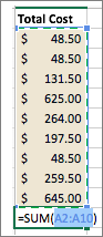
One quick and easy way to add values in Excel is to use AutoSum. Just select an empty cell directly below a column of data. Then on the Formula tab, click AutoSum > Sum. Excel will automatically sense the range to be summed. (AutoSum can also work horizontally if you select an empty cell to the right of the cells to be summed.)

AutoSum creates the formula for you, so that you don’t have to do the typing. However, if you prefer typing the formula yourself, see the SUM function.

Add based on conditions

Use the SUMIF function when you want to sum values with one condition. For example, when you need to add up the total sales of a certain product.

Use the SUMIFS function when you want to sum values with more than one condition. For instance, you might want to add up the total sales of a certain product, within a certain sales region.

Add or subtract dates

For an overview of how to add or subtract dates, see Add or subtract dates. For more complex date calculations, see Date and time functions.

Add or subtract time

For an overview of how to add or subtract time, see Add or subtract time. For other time calculations, see Date and time functions.

Need more help?

You can always ask an expert in the Excel Tech Community or get support in the Answers community.

Источник

Add and subtract numbers

Adding and subtracting in Excel is easy; you just have to create a simple formula to do it. Just remember that all formulas in Excel begin with an equal sign (=), and you can use the formula bar to create them.

Add two or more numbers in one cell

Click any blank cell, and then type an equal sign ( =) to start a formula.

After the equal sign, type a few numbers separated by a plus sign (+).

For example, 50+10+5+3.

If you use the example numbers, the result is 68.

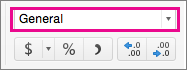
If you see a date instead of the result that you expected, select the cell, and then on the Home tab, select General.

Add numbers using cell references

A cell reference combines the column letter and row number, such as A1 or F345. When you use cell references in a formula instead of the cell value, you can change the value without having to change the formula.

Type a number, such as 5, in cell C1. Then type another number, such as 3, in D1.

In cell E1, type an equal sign ( =) to start the formula.

After the equal sign, type C1+D1.

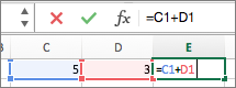
If you use the example numbers, the result is 8.

If you change the value of C1 or D1 and then press RETURN , the value of E1 will change, even though the formula did not.

If you see a date instead of the result that you expected, select the cell, and then on the Home tab, select General.

Get a quick total from a row or column

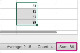
Type a few numbers in a column, or in a row, and then select the range of cells that you just filled.

On the status bar, look at the value next to Sum. The total is 86.

Subtract two or more numbers in a cell

Click any blank cell, and then type an equal sign ( =) to start a formula.

After the equal sign, type a few numbers that are separated by a minus sign (-).

For example, 50-10-5-3.

If you use the example numbers, the result is 32.

Subtract numbers using cell references

Type a number in cells C1 and D1.

For example, a 5 and a 3.

In cell E1, type an equal sign ( =) to start the formula.

After the equal sign, type C1-D1.

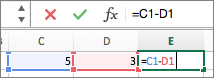
If you used the example numbers, the result is 2.

If you change the value of C1 or D1 and then press RETURN , the value of E1 will change, even though the formula did not.

If you see a date instead of the result that you expected, select the cell, and then on the Home tab, select General.

Add two or more numbers in one cell

Click any blank cell, and then type an equal sign ( =) to start a formula.

After the equal sign, type a few numbers separated by a plus sign (+).

For example, 50+10+5+3.

If you use the example numbers, the result is 68.

Note: If you see a date instead of the result that you expected, select the cell, and then on the Home tab, under Number, click General on the pop-up menu.

Add numbers using cell references

Type a number, such as 5, in cell C1. Then type another number, such as 3, in D1.

In cell E1, type an equal sign ( =) to start the formula.

After the equal sign, type C1+D1.

If you use the example numbers, the result is 8.

If you change the value of C1 or D1 and then press RETURN , the value of E1 will change, even though the formula did not.

If you see a date instead of the result that you expected, select the cell, and then on the Home tab, under Number, click General on the pop-up menu.

Get a quick total from a row or column

Type a few numbers in a column, or in a row, and then select the range of cells that you just filled.

On the status bar, look at the value next to Sum=. The total is 86.

If you don’t see the status bar, on the View menu, click Status Bar.

Subtract two or more numbers in a cell

Click any blank cell, and then type an equal sign ( =) to start a formula.

After the equal sign, type a few numbers that are separated by a minus sign (-).

For example, 50-10-5-3.

If you use the example numbers, the result is 32.

Subtract numbers using cell references

Type a number in cells C1 and D1.

For example, a 5 and a 3.

In cell E1, type an equal sign ( =) to start the formula.

After the equal sign, type C1-D1.

If you used the example numbers, the result is -2.

If you change the value of C1 or D1 and then press RETURN , the value of E1 will change, even though the formula did not.

If you see a date instead of the result that you expected, select the cell, and then on the Home tab, under Number, click General on the pop-up menu.

Источник

Automatically number rows

Unlike other Microsoft 365 programs, Excel does not provide a button to number data automatically. But, you can easily add sequential numbers to rows of data by dragging the fill handle to fill a column with a series of numbers or by using the ROW function.

Tip: If you are looking for a more advanced auto-numbering system for your data, and Access is installed on your computer, you can import the Excel data to an Access database. In an Access database, you can create a field that automatically generates a unique number when you enter a new record in a table.

What do you want to do?

Fill a column with a series of numbers

Select the first cell in the range that you want to fill.

Type the starting value for the series.

Type a value in the next cell to establish a pattern.

Tip: For example, if you want the series 1, 2, 3, 4, 5. type 1 and 2 in the first two cells. If you want the series 2, 4, 6, 8. type 2 and 4.

Select the cells that contain the starting values.

Note: In Excel 2013 and later, the Quick Analysis button is displayed by default when you select more than one cell containing data. You can ignore the button to complete this procedure.

Drag the fill handle across the range that you want to fill.

Note: As you drag the fill handle across each cell, Excel displays a preview of the value. If you want a different pattern, drag the fill handle by holding down the right-click button, and then choose a pattern.

To fill in increasing order, drag down or to the right. To fill in decreasing order, drag up or to the left.

Tip: If you do not see the fill handle, you may have to display it first. For more information, see Display or hide the fill handle.

Note: These numbers are not automatically updated when you add, move, or remove rows. You can manually update the sequential numbering by selecting two numbers that are in the right sequence, and then dragging the fill handle to the end of the numbered range.

Use the ROW function to number rows

In the first cell of the range that you want to number, type =ROW(A1).

The ROW function returns the number of the row that you reference. For example, =ROW(A1) returns the number 1.

Drag the fill handle across the range that you want to fill.

Tip: If you do not see the fill handle, you may have to display it first. For more information, see Display or hide the fill handle.

These numbers are updated when you sort them with your data. The sequence may be interrupted if you add, move, or delete rows. You can manually update the numbering by selecting two numbers that are in the right sequence, and then dragging the fill handle to the end of the numbered range.

If you are using the ROW function, and you want the numbers to be inserted automatically as you add new rows of data, turn that range of data into an Excel table. All rows that are added at the end of the table are numbered in sequence. For more information, see Create or delete an Excel table in a worksheet.

To enter specific sequential number codes, such as purchase order numbers, you can use the ROW function together with the TEXT function. For example, to start a numbered list by using 000-001, you enter the formula =TEXT(ROW(A1),»000-000″) in the first cell of the range that you want to number, and then drag the fill handle to the end of the range.

Display or hide the fill handle

The fill handle displays by default, but you can turn it on or off.

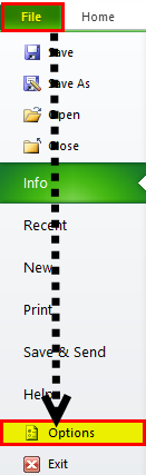
In Excel 2010 and later, click the File tab, and then click Options.

In Excel 2007, click the Microsoft Office Button , and then click Excel Options.

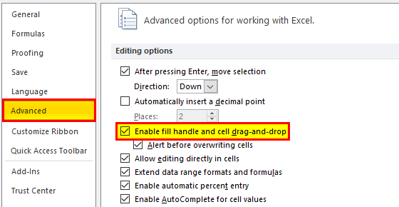
In the Advanced category, under Editing options, select or clear the Enable fill handle and cell drag-and-drop check box to display or hide the fill handle.

Note: To help prevent replacing existing data when you drag the fill handle, ensure the Alert before overwriting cells check box is selected. If you do not want Excel to display a message about overwriting cells, you can clear this check box.

Источник

Use AutoSum to sum numbers

If you need to sum a column or row of numbers, let Excel do the math for you. Select a cell next to the numbers you want to sum, click AutoSum on the Home tab, press Enter, and you’re done.

When you click AutoSum, Excel automatically enters a formula (that uses the SUM function) to sum the numbers.

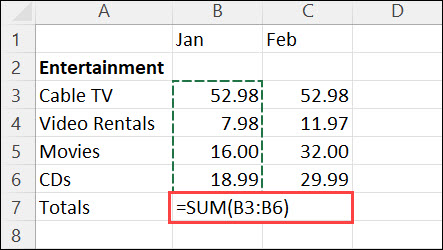
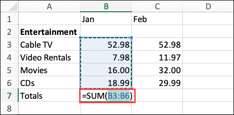
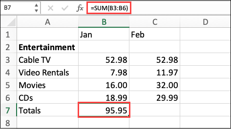
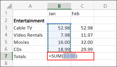
Here’s an example. To add the January numbers in this Entertainment budget, select cell B7, the cell immediately below the column of numbers. Then click AutoSum. A formula appears in cell B7, and Excel highlights the cells you’re totaling.

AutoSum» loading=»lazy»>

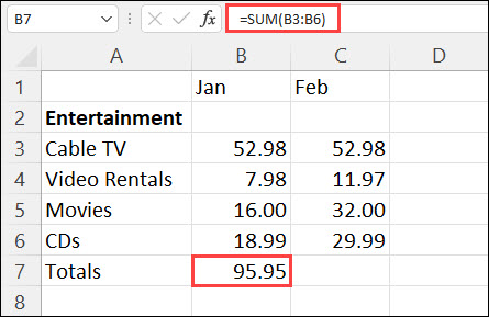
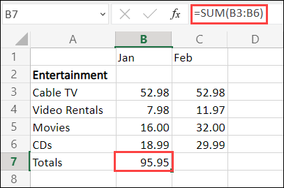
Press Enter to display the result (95.94) in cell B7. You can also see the formula in the formula bar at the top of the Excel window.

To sum a column of numbers, select the cell immediately below the last number in the column. To sum a row of numbers, select the cell immediately to the right.

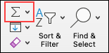
AutoSum is in two locations: Home > AutoSum, and Formulas > AutoSum.

Once you create a formula, you can copy it to other cells instead of typing it over and over. For example, if you copy the formula in cell B7 to cell C7, the formula in C7 automatically adjusts to the new location, and calculates the numbers in C3:C6.

You can also use AutoSum on more than one cell at a time. For example, you could highlight both cell B7 and C7, click AutoSum, and total both columns at the same time.

You can also sum numbers by creating a simple formula.

If you need to sum a column or row of numbers, let Excel do the math for you. Select a cell next to the numbers you want to sum, click AutoSum on the Home tab, press Enter, and you’re done.

When you click AutoSum, Excel automatically enters a formula (that uses the SUM function) to sum the numbers.

Press Enter to display the result (95.94) in cell B7. You can also see the formula in the formula bar at the top of the Excel window.

To sum a column of numbers, select the cell immediately below the last number in the column. To sum a row of numbers, select the cell immediately to the right.

AutoSum is in two locations: Home > AutoSum, and Formulas > AutoSum.

You can also use AutoSum on more than one cell at a time. For example, you could highlight both cell B7 and C7, click AutoSum, and total both columns at the same time.

You can also sum numbers by creating a simple formula.

On your Android tablet or Android phone

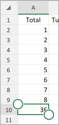
In a worksheet, tap the first empty cell after a range of cells that has numbers, or tap and drag to select the range of cells you want to calculate.

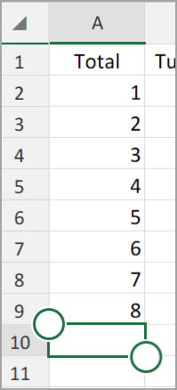
Tap the check mark.

If you need to sum a column or row of numbers, let Excel do the math for you. Select a cell next to the numbers you want to sum, click AutoSum on the Home tab, press Enter, and you’re done.

When you click AutoSum, Excel automatically enters a formula (that uses the SUM function) to sum the numbers.

Press Enter to display the result (95.94) in cell B7. You can also see the formula in the formula bar at the top of the Excel window.

To sum a column of numbers, select the cell immediately below the last number in the column. To sum a row of numbers, select the cell immediately to the right.

AutoSum is in two locations: Home > AutoSum, and Formulas > AutoSum.

You can also use AutoSum on more than one cell at a time. For example, you could highlight both cell B7 and C7, click AutoSum, and total both columns at the same time.

You can also sum numbers by creating a simple formula.

Need more help?

You can always ask an expert in the Excel Tech Community or get support in the Answers community.

Источник

Excel for Microsoft 365 for Mac Excel 2021 for Mac Excel 2019 for Mac Excel 2016 for Mac Excel for Mac 2011 More…Less

Add two or more numbers in one cell

Click any blank cell, and then type an equal sign (=) to start a formula.
After the equal sign, type a few numbers separated by a plus sign (+).

For example, 50+10+5+3.
Press RETURN .

If you use the example numbers, the result is 68.
Notes:
- If you see a date instead of the result that you expected, select the cell, and then on the Home tab, select General.

Add numbers using cell references

Type a number, such as 5, in cell C1. Then type another number, such as 3, in D1.
In cell E1, type an equal sign (=) to start the formula.
After the equal sign, type C1+D1.
Press RETURN .

If you use the example numbers, the result is 8.
Notes:
- If you change the value of C1 or D1 and then press RETURN , the value of E1 will change, even though the formula did not.
- If you see a date instead of the result that you expected, select the cell, and then on the Home tab, select General.

Get a quick total from a row or column

Type a few numbers in a column, or in a row, and then select the range of cells that you just filled.
On the status bar, look at the value next to Sum. The total is 86.

Subtract two or more numbers in a cell

Click any blank cell, and then type an equal sign (=) to start a formula.
After the equal sign, type a few numbers that are separated by a minus sign (-).

For example, 50-10-5-3.
Press RETURN .

If you use the example numbers, the result is 32.

Subtract numbers using cell references

Type a number in cells C1 and D1.

For example, a 5 and a 3.
In cell E1, type an equal sign (=) to start the formula.
After the equal sign, type C1-D1.
Press RETURN .

If you used the example numbers, the result is 2.
Notes:
- If you change the value of C1 or D1 and then press RETURN , the value of E1 will change, even though the formula did not.
- If you see a date instead of the result that you expected, select the cell, and then on the Home tab, select General.

Add two or more numbers in one cell

Click any blank cell, and then type an equal sign (=) to start a formula.
After the equal sign, type a few numbers separated by a plus sign (+).

For example, 50+10+5+3.
Press RETURN .

If you use the example numbers, the result is 68.

Note: If you see a date instead of the result that you expected, select the cell, and then on the Home tab, under Number, click General on the pop-up menu.

Add numbers using cell references

Type a number, such as 5, in cell C1. Then type another number, such as 3, in D1.
In cell E1, type an equal sign (=) to start the formula.
After the equal sign, type C1+D1.
Press RETURN .

If you use the example numbers, the result is 8.
Notes:
- If you change the value of C1 or D1 and then press RETURN , the value of E1 will change, even though the formula did not.
- If you see a date instead of the result that you expected, select the cell, and then on the Home tab, under Number, click General on the pop-up menu.

Get a quick total from a row or column

Type a few numbers in a column, or in a row, and then select the range of cells that you just filled.
On the status bar, look at the value next to Sum=. The total is 86.

If you don’t see the status bar, on the View menu, click Status Bar.

Subtract two or more numbers in a cell

Click any blank cell, and then type an equal sign (=) to start a formula.
After the equal sign, type a few numbers that are separated by a minus sign (-).

For example, 50-10-5-3.
Press RETURN .

If you use the example numbers, the result is 32.

Subtract numbers using cell references

Type a number in cells C1 and D1.

For example, a 5 and a 3.
In cell E1, type an equal sign (=) to start the formula.
After the equal sign, type C1-D1.
Press RETURN .

If you used the example numbers, the result is -2.
Notes:
- If you change the value of C1 or D1 and then press RETURN , the value of E1 will change, even though the formula did not.
- If you see a date instead of the result that you expected, select the cell, and then on the Home tab, under Number, click General on the pop-up menu.

Simple addition

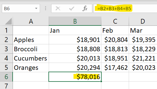
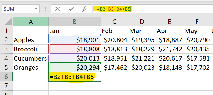
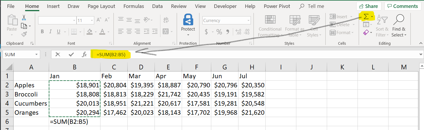
In the example below we have a list of cells containing the amount of money in sales for 12 months for 4 products. Assuming that we want to add all the amounts in January, let’s do a simple addition of the 4 numbers highlighted.

How to create a simple addition

A simple addition looks like this: Total = B2 + B3+ B4+ B5

The Excel Formula is built as you type or as you select each cell to be added.

How to build up the addition formula

Here are the steps:

type =
select B2
type +
select B3
type +
select B4
type +
select B5
Type Enter

Alternatively, you can type the entire formula using your keyboard

=B2+B3+B4+B5 (type Enter to calculate the formula)

Notice how the cells in the formula are highlighting as you type. To identify the cells, Excel uses a different color for each one.

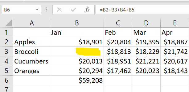
When you press Enter, the formula is calculating the result and Excel is displaying it in the B6 cell (or wherever you typed the formula):

What happens when you add empty cells

If one or more of the cells are empty, Excel will consider them zero.

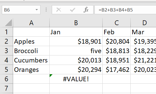
What happens if you add cells that are not numbers

If one or more of the cells are not a number, the formula will result in an error

As any Excel formulas, the result will always show the current value of the addition of these cells.

Any time you change one of the values in the added cells, the result will change immediately to show the correct sum of these cells.

How to build the formula using the mouse

Here is how you do the addition using the mouse to point at the cells as you add.

Click on the cell where you want the result of the calculation to appear (B6)
Type = (press the “equals” (=) key to start writing your formula)
Click on the first cell to be added (B2)
Type + (that’s the plus sign)
Click on the second cell to be added (B3)
Type + again, and the next cell to be added.
Repeat until all cells to be added have been clicked.
Press Enter.

This will create the same addition formula as above without the manual typing.

Only use this approach for a limited number of cells due to the difficulty of keeping track of all the cells to be added.
Use the next method (the SUM() function) for a larger set of numbers.

Use the SUM() function to add up numbers in a column

The SUM() function is a more efficient way to add up cells.

You can use the SUM function to add up individual cells, or to add up a range of cells simply by specifying the first and last cell in a range of cells to be added up.

The SUM() function will add up the values in all the cells between the start cell and the end cell in the shortest path possible.

It becomes very useful when adding hundreds, or thousands of cells. Excel has over 1,000,000 rows so imaging typing that many cells into an addition. It is much easier to type a formula like SUM (A1:A1000000)

How to use the SUM() function

If you look at the earlier example, you could use SUM() as shown in the screenshot to achieve the same result.

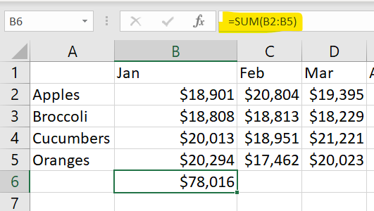
Notice how the cells included in the formula are highlighted just like in the addition case above.

However, in this case, a range is highlighted from the first cell to the last cell specified. This is a useful way to check whether your formula is using the correct range for the SUM.

This formula adds up all the cells from B2 to B5 inclusive. This method can be used just as easily to add up several thousands of cells in a row or column, as well as a set of rows or a set of columns.

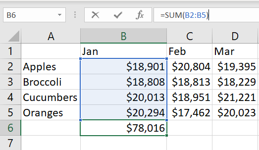
Add numbers in a column (B2 to B5)

In the example below, the SUM function is adding numbers in a column. As you type the formula, observe the blue mark showing you the range that is added.

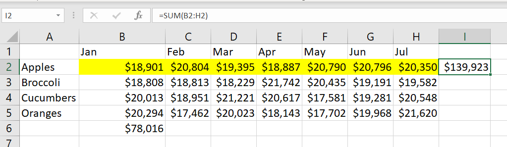
Add numbers in a row (B2 to H2)

In the screenshot below, the same function can be used to sum up the values in a row.

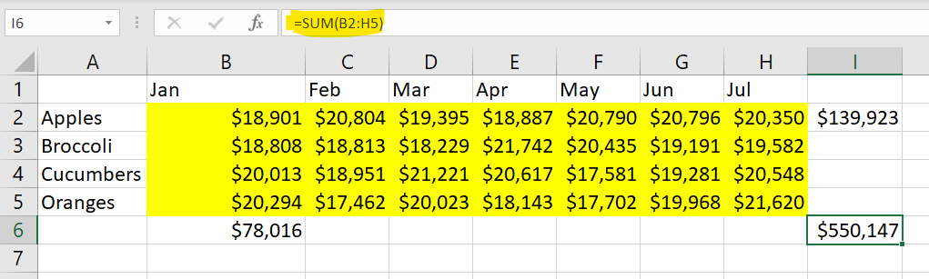
Several rows and columns (all rows and columns B2 to H5)

In the next example, Excel is adding all the values in an array.

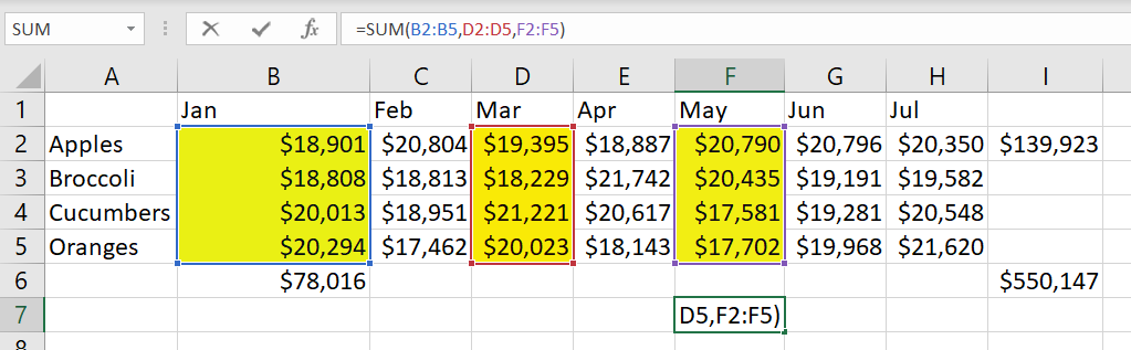
Multiple ranges

You can use SUM to add numbers in multiple ranges (only the months of January, March and May). Press CTRL while selecting all the ranges needed with the mouse.

While you type, notice the Range is highlighted so that you are aware of what is being added in the formula.

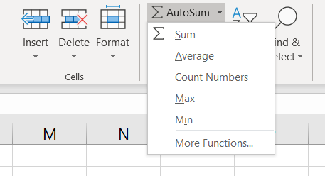
The AUTOSUM button

The last and most efficient method to sum up numbers in a row or column is to use the AUTOSUM button.

This button will use Excel artificial intelligence to evaluate your data set. If your selection is on the first empty cell under a column when you press the AUTOSUM button, Excel will assume that you want to add all the numbers in that column and place the result in the empty cell. This is what 99% of users do. This method saves even more time in typing additions or SUM formulas but just pressing one button.

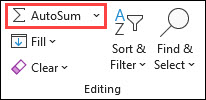
Where can I find the AUTOSUM button

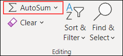
Autosum is in the Home tab, in the Editing subsection

Modify the resulting formula as you like to reduce or increase the range of numbers.

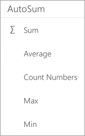
There are other function under the Autosum dropdown that you can use. You can calculate the average of your numbers, count them, pick the minimum or the maximum and even explore other numerical functions.

These are the three ways Excel can add numbers on a column or row.

Источник

While editing a spreadsheet in Microsoft Excel, you may encounter a situation which requires you to add a number to all cells in a column or a table. Doing the calculation manually and filling the cells one by one is apparently not the best idea. In fact, you can use Paste Special to achieve this goal within a very short time.

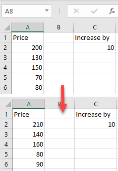
For example, now I want to add 30 to the scores of all the students in column C.

Enter the number 30 in any of the cells beside column C.

Press Ctrl+C to select this cell or right-click it and click Copy in the menu. Then select all the scores in column C.

Switch to Home tab and click Paste – Paste Special… or right-click the selected cells in column C and choose Paste Special under Paste Options.

Choose Add in Operation in the popping out Paste Special window. Then hit OK to implement it.

This number you entered will be added to all the cells in column C right away.

Copyright Statement: Regarding all of the posts by this website, any copy or use shall get the written permission or authorization from Myofficetricks.

Источник

I have column in Excel colA. I want to add a number ,say 2000 , to all values in cell under colA . How can i do this ? The SUM function ends up totaling all the values on giving range of cells and the number to be added .

colA
----
8001
8002
8003
8004
8005

What I want

colA
----
10000
10001
10002
10003
10004

How to place formula on selected the cells ? Please help.

asked Sep 25, 2012 at 5:52

Mudassir HasanMudassir Hasan

27.8k19 gold badges100 silver badges130 bronze badges

Enter 2000 into any cell and copy it, then highlight the column that you want to add to and use Paste Special -> Add.

answered Sep 25, 2012 at 5:55

Источник

Download Article

Numbering Rows Dynamically

Filling a Column with Continuous Numbers

Video

Tips

Warnings

Adding numbers automatically to a column in Excel can be done in two ways, using the ROW function or the Fill feature. The first method ensures that the cells display the correct row numbers even when rows are added or deleted. The second, and easier method, works just as well but you’ll need to redo it whenever you add or delete a row in order to keep the numbers accurate. The method you choose is based on your comfort with using Excel and what you’re using the application for, but each one is straightforward and will have your sheet organized in no time.

1
Click the first cell where the series of numbers will begin. This method explains how to make each cell in a column display its corresponding row number.^[1] This is a good method to use if rows are frequently added and removed in your worksheet.
- To create a basic row of consecutive numbers (or other data, such as days of the week or months of the year), see Filling a Column with Continous Numbers.
2
Type =ROW(A1) into the cell (if it is cell A1). If the cell is not A1, use the correct cell number.
- For example, if you are typing in cell B5, type =ROW(B5) instead.
Advertisement
3
Press ↵ Enter. The cell will now display its row number. If you typed =ROW(A1), the cell will say 1. If you typed =ROW(B5), the cell will read 5.^[2]
- To start with 1 no matter which row you want to begin your series of numbers, count the number of rows above your current cell, then subtract that number from your formula.
- For example, if you entered =ROW(B5) and want the cell to display a 1, edit the formula to say =ROW(B5)-4, as B1 is back 4 rows from B5.^[3]
4

Select the cell containing the first number in the series.
5
Hover the cursor over the box at the bottom right corner of the selected cell. This box is called the Fill Handle. When the mouse cursor is directly above the Fill Handle, the cursor will change to a crosshair symbol.
- If you don’t see the Fill Handle, navigate to File > Options > Advanced and place a check next to “Enable fill handle and cell drag-and-drop.”
6
Drag the Fill Handle down to the final cell in your series. The cells in the column will now display their corresponding row numbers.
- If you delete a row included in this series, the cells numbers will automatically correct themselves based on their new row numbers.

1
Click the cell where your series of numbers will begin. This method will show you how to add a series of continuous numbers to the cells in a column.
- If you use this method and later have to delete a row, you will need to repeat the steps to renumber the entire column. If you think you will be manipulating rows of data often, see Numbering Rows instead.
2
Type the first number of your series into the cell. For instance, if you will be numbering entries down a column, type 1 into this cell.
- You don’t have to start with 1. Your series can start at any number, and can even follow other patterns (such as even numbers, in multiples of 5, and more).
- Excel also supports other types “numbering,” including dates, seasons, and days of the week. To fill a column with the days of the week, for example, the first cell should say “Monday.”
3

Click the next cell in the pattern. This should be the cell directly beneath the currently active cell.
4
Type the second number of the series to create the pattern. To number consecutively (1, 2, 3, etc), type a 2 here.^[4]
- If you wanted your continuous numbers to be something like 10, 20, 30, 40, etc, the first two cells in the series should be 10 and 20.
- If you are using days of the week, type the next day of the week into the cell.
5

Click and drag to select both cells. When you release the mouse button, the both cells will be highlighted.
6
Hover the cursor over the tiny box at the bottom right corner of the highlighted area. This box is called the Fill Handle. When the mouse pointer is directly on top of the Fill Handle, the cursor will become a crosshair symbol.
- If you don’t see the Fill Handle, navigate to File > Options > Advanced and place a check next to “Enable fill handle and cell drag-and-drop.”
7

Click and drag the Fill Handle down to the final cell in your desired series. Once you release the mouse button, the cells in the column will be numbered according to the pattern you established in the first two cells.

Add New Question

Question

Why does Autonumber repeat the sequence rather than fill down when I drag down?

After dragging down, there is an icon next to the last cell that gives you options of whether you want to copy cells or fill series. Click the intended option.

Ask a Question

200 characters left

Include your email address to get a message when this question is answered.

Submit

Video

Microsoft provides a free online version of Excel as a part of Microsoft Office Online.
You can also open and edit your spreadsheets in Google Sheets.

Thanks for submitting a tip for review!

Always make sure the «Alert before overwriting cells» option is checked in the Advanced tab of Excel Options. This will help prevent data entry errors and the need to recreate formulas or other data.

About This Article

Article SummaryX

1. Type » =ROW(A1)» into the first cell (if the cell is A1).
2. Press Enter.
3. Select the cell.
4. Drag the fill handle to the final cell in the series.

Did this summary help you?

Thanks to all authors for creating a page that has been read 467,700 times.

Is this article up to date?

Источник

See all How-To Articles

This tutorial demonstrates how to add values to cells and columns in Excel and Google Sheets.

Add Values to Multiple Cells

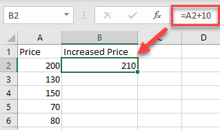
To add a value to a range of cells, click on the cell where you want to display the result, and enter = (equal) and the cell reference of the first number then + (plus) and the number you want to add.

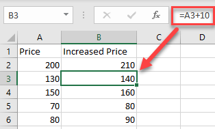
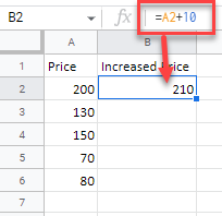
For this example, start with cell A2 (200). Cell B2 will show the Price in A2 increased by 10. So, in cell B2, enter:

=A2+10

As a result, the value in cell B2 is now 210 (value from A2 plus 10).

Now copy this formula down the column to the rows below. Click on the cell where you entered the formula (F2) and place your cursor on the bottom right corner of the cell.
When it changes to a plus sign, drag it down to the rest of the rows where you want to apply the formula (here, B2:B6).

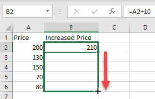
As a result of relative cell referencing, the constant (here, 10) remains the same, but the cell address changes according to the row you are in (so B3=A3+10, and so on).

Add Multiple Cells With Paste Special

You can also add a number to multiple cells and return the result as a number in the same cell.

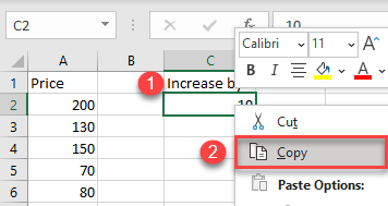
First, select the cell with the value you want to add (here, cell C2), right-click, and from the drop-down menu, choose Copy (or use the shortcut CTRL + C).

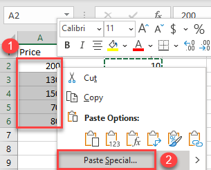
After that, select the cells where you want to subtract the value and right-click on the data range (here, A2:A6). In the drop-down menu, click on Paste Special.

The Paste Special window will appear. Under the Operation section choose Add, and then click OK.

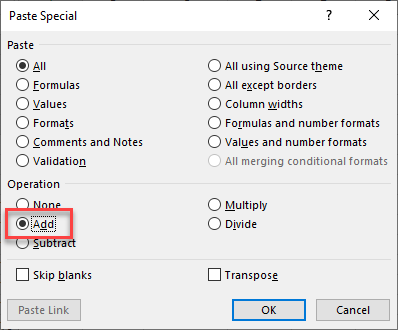
You’ll see the result as a number within the same cells. (In this example, 10 was added to each value from the data range A2:A6.) This method is better if you don’t want to display the results in a new column and don’t need to retain a record of the original values.

Add Column With Cell References

To add an entire column to another using cell references, select the cell where you want to display the result, and enter = (equal) and the cell reference for the first number then + (plus) and the reference for the cell you want to add.

For this example, calculate the summary of Price 1 (A2) and Price 2 (B2). So, in cell C2, enter:

=A2+B2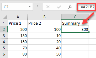

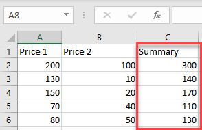
To apply the formula to an entire column, just copy the formula down to the rest of the rows in the table (here, C2:C6).

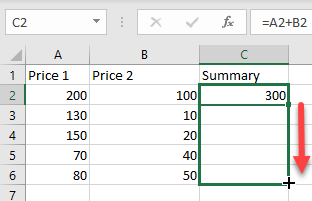
Now, you have a new column with the summary.

Using the methods above, you can also subtract, multiply, or divide cells and columns in Excel.

Add Cells and Columns in Google Sheets

In Google Sheets, you can add multiple cells using formulas in exactly the same ways as in Excel; except, you can’t use Paste Special.

Источник

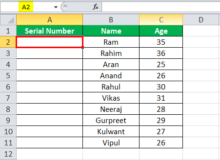
While performing a simple numbering in Excel, we manually provide a cell number for the serial number; we can also do it automatically. To do auto numbering, we have two methods. First, we can fill the first two cells with the series of the number we want to be inserted and drag it down to the end of the table. The second method is to use the =ROW () formula which will give us the number, and then drag the formula similar to the end of the table.

For example, suppose you have a data set and want to start numbering them from 3 and step up by 4 until 40. First, you may select the cells containing the 3 and the 7. Then, click on the handle and drag to the other cells where you can see 40. You may then release and view that the numbers are filled in automatically.

You may also use the Excel ROW function = ROW() formula that returns the row number for reference. For example, ROW(A3) returns 3 as A3 is the third row in the spreadsheet. If not given any reference, ROW returns the cell’s row number, which consists of the formula.

Automatic Numbering in Excel

Numbering means giving serial numbers or numbers to a list of data. In Excel, no special button is provided that offers numbering for our data. As we already know, Excel does not provide a method, tool, or button to provide the sequential number to a list of data, which means we need to do it manually.

Automatic Numbering in Excel
- How to Auto Number in Excel?
- Top 3 ways to get Auto Numbering in Excel
  - #1 – Filling the Column with a Series of Numbers
  - #2 – Use ROW() Function
  - #3 – Using Offset() Function
- Things to Remember about Auto Numbering in Excel
- Auto Numbering in Excel Video
- Recommended Articles

How to Auto Number in Excel?

We must remember that our AutoFill functionAutoFill in excel can fill a range in a specific direction by using the fill handle.read more is always turned on to create auto numbering in Excel. By default, it is turned on. But in any case, if it is not enabled or mistakenly disabled “AutoFill,” here is how we can re-enable it.

Now we have checked that the “Autofill” is enabled. There are three methods for Excel auto-numbering:

Fill a column with a series of numbers.
Using the Row() function.
Using the Offset() function.

The following are the steps for enabling fill handle and cell drag and drop: –

In the “File” tab, go to “Options.”
In the advanced section, check the “Enable fill handle and cell drag and drop” in Excel under the editing options.

Top 3 ways to get Auto Numbering in Excel

There are various ways to get automatic numbering in Excel.

You can download this Auto Numbering Excel Template here – Auto Numbering Excel Template

Fill a column with a series of numbers.
Use Row() function
Use Offset() Function

Let us discuss all the above methods by examples.

#1 – Filling the Column with a Series of Numbers

We have the following data:

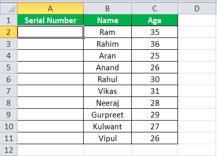
We will insert automatic numbers in Excel “column A” following the below steps:

We can select the cell we want to fill. In this example, we will choose cell A2.
We will write the number we want to start with. Let it be 1, fill the next cell in the same column with another number, and let it be 2.

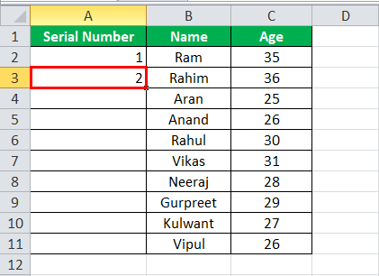
To start a pattern, we have made the numbering 1 in cell A2 and 2 in cell A3. Next, we will select the starting values, i.e., cells A2 and A3.

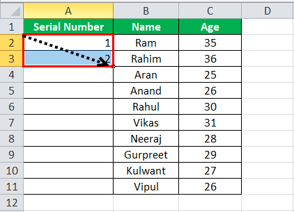
The arrow shows the pointer (dot) in the selected cell. Then, click on it and drag it to the desired range, cell A11.

Now, we have sequential numbering for our data.

#2 – Use ROW() Function

We will use the same data to demonstrate the sequential numbering by the Row() functionThe row function in Excel is a worksheet function that displays the current row index number of the selected or target cell. The syntax to use this function is as follows: =ROW( Value ).read more.

Below is our data:

We select the specific cell where we want to start our automatic numbering in Excel (cell A2 in this case).

We type ROW() in cell A2 and press “Enter.”

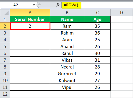
As a result, it gave us the numbering from number 2 since the Row function throws the number for the current row.

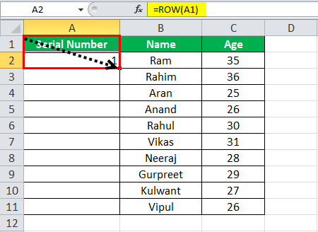
To avoid the above situation, we can give the reference row to the Row function.

Next, we click on the pointer or the dot in the selected cell and drag it to the desired range for the current scenario to cell A11.

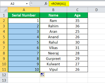
We have automatic numbering in Excel for the data using the Row() function.

#3 – Using Offset() Function

We can also achieve auto numbering in Excel using the Offset() functionThe OFFSET function in excel returns the value of a cell or a range (of adjacent cells) which is a particular number of rows and columns from the reference point. read more also.

Let us use the same data to demonstrate the Offset function. Below is the data:

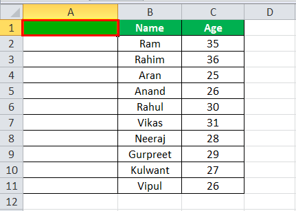
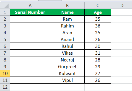
As we can see, we have removed the text written in cell A1 “Serial Number,” as the reference needs to be blank while using the Offset function.

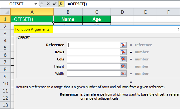
The above screenshot shows the function arguments used in the Offset function.

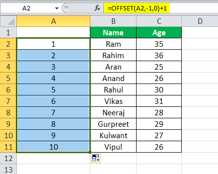
In cell A2, we type offset(A2,-1,0)+1 for the automatic numbering in Excel.

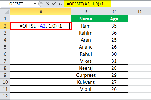
A2 is the current cell address, which is the reference.

Press the “Enter” key. It will insert the first number.

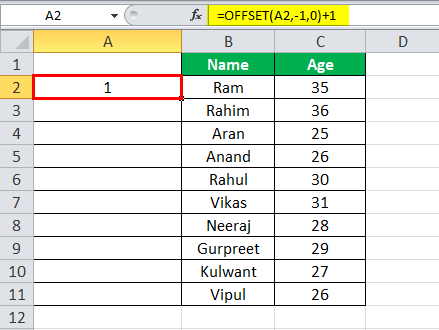
Now, we select cell A2 and drag it down to cell A11.

So, now we have sequential numbering using the Offset function.

Things to Remember about Auto Numbering in Excel

Excel does not auto-provide auto-numbering.
Do not forget to check for the enabled “AutoFill” option.
While filling a column with a series of numbers, we must make a pattern. We can use the starting values as 2 or 4 to create even sequential numbering.

Auto Numbering in Excel Video

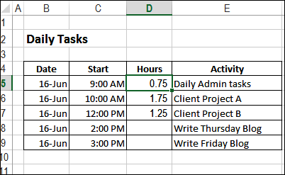
Daily To Do List

In this example, I keep track of my To Do list in a workbook, and one of my items is “Daily Admin tasks”. Sometimes, I start the day by answering client emails, posting links to my latest blog post, and doing the accounting for the previous day’s sales.

So, I enter the time spent – 0.75 hours – and move on to the next task.

Later in the day, I might spend another 45 minutes on Admin tasks, so I want to add that to the previous amount, in cell D5.
If it’s late in the day, it might be difficult to add 0.75 + 0.75 in my head (or early in the day, if I haven’t had my coffee yet!)

Use Paste Special

One way to do this, and avoid basic mistakes in arithmetic, is to use Paste Special – Add.

Type the number in a cell, and copy that cell.
Then, use Paste Special – Add, to paste that amount into another cell.

In the screen shot below, I’ve selected the Add operation in the Paste Special dialog box.

That technique works well, but it takes a few steps – and that adds more time to my Admin tasks!

Use a Macro to Add Amounts

To make the job easier, I created a couple of macros that add numbers to selected cells. There is a link to the download page, at the end of this article.

Macro 1 adds a set number to the selected cells.
Macro 2 asks you to enter a number, then adds that number to the selected cells.

In the macro code, I use 7 as the set number, and the default number, because I have several weekly tasks. Once they’re completed, I add 7 to the date, to move them to next week’s schedule.

You could change the code, so the set/default number is something that you use frequently.

Video: Add Numbers to Multiple Cells in Excel

Watch this video to see how to use the Paste Special command, and see how to modify the macro code, to change the numbers.

Video Timeline

00:00 Introduction
00:33 Manually Add Number
01:23 Macro 1: Add Specific Number
02:07 Macro 2: Prompt for Number
02:44 See the Macro 2 Code
03:22 Modify the Macro Code
04:14 See the Macro 1 Code
04:34 Macro Buttons
04:52 Get the Sample File

Download the Sample File

To see how the macros work, and get the code to use in your own Microsoft Excel worksheet, you can visit my Contextures website. You’ll find the instructions and sample file on the Add Number to Multiple Cells page.

The zipped file is in xlsm format, and contains macros. Enable macros when you open the file, if you want to test the code.
____________________

Источник

Add a list of numbers in a column

Ways to add values in a spreadsheet

Add based on conditions

Add or subtract dates

Add or subtract time

Need more help?

Add and subtract numbers

Add two or more numbers in one cell

Add numbers using cell references

Get a quick total from a row or column

Subtract two or more numbers in a cell

Subtract numbers using cell references

Add two or more numbers in one cell

Add numbers using cell references

Get a quick total from a row or column

Subtract two or more numbers in a cell

Subtract numbers using cell references

Automatically number rows

What do you want to do?

Fill a column with a series of numbers

Use the ROW function to number rows

Display or hide the fill handle

Use AutoSum to sum numbers

On your Android tablet or Android phone

Need more help?

Add two or more numbers in one cell

Add numbers using cell references

Get a quick total from a row or column

Subtract two or more numbers in a cell

Subtract numbers using cell references

Add two or more numbers in one cell

Add numbers using cell references

Get a quick total from a row or column

Subtract two or more numbers in a cell

Subtract numbers using cell references

See also

Need more help?

Simple addition

How to create a simple addition

How to build up the addition formula

What happens when you add empty cells

What happens if you add cells that are not numbers

How to build the formula using the mouse

Use the SUM() function to add up numbers in a column

How to use the SUM() function

Add numbers in a column (B2 to B5)

Add numbers in a row (B2 to H2)

Several rows and columns (all rows and columns B2 to H5)

Multiple ranges

The AUTOSUM button

Where can I find the AUTOSUM button

Video

About This Article

Is this article up to date?

Add Values to Multiple Cells

Add Multiple Cells With Paste Special

Add Column With Cell References

Add Cells and Columns in Google Sheets

Automatic Numbering in Excel

Table of contents

How to Auto Number in Excel?

Top 3 ways to get Auto Numbering in Excel

#1 – Filling the Column with a Series of Numbers

#2 – Use ROW() Function

#3 – Using Offset() Function

Things to Remember about Auto Numbering in Excel

Auto Numbering in Excel Video

Recommended Articles

Daily To Do List

Use Paste Special

Use a Macro to Add Amounts

Video: Add Numbers to Multiple Cells in Excel

Download the Sample File