
Excel for Microsoft 365 Excel 2021 Excel 2019 Excel 2016 Excel 2013 Excel 2010 Excel 2007 More…Less
In Excel, formatting worksheet (or sheet) data is easier than ever. You can use several fast and simple ways to create professional-looking worksheets that display your data effectively. For example, you can use document themes for a uniform look throughout all of your Excel spreadsheets, styles to apply predefined formats, and other manual formatting features to highlight important data.
A document theme is a predefined set of colors, fonts, and effects (such as line styles and fill effects) that will be available when you format your worksheet data or other items, such as tables, PivotTables, or charts. For a uniform and professional look, a document theme can be applied to all of your Excel workbooks and other Office release documents.
Your company may provide a corporate document theme that you can use, or you can choose from a variety of predefined document themes that are available in Excel. If needed, you can also create your own document theme by changing any or all of the theme colors, fonts, or effects that a document theme is based on.
Before you format the data on your worksheet, you may want to apply the document theme that you want to use, so that the formatting that you apply to your worksheet data can use the colors, fonts, and effects that are determined by that document theme.
For information on how to work with document themes, see Apply or customize a document theme.
A style is a predefined, often theme-based format that you can apply to change the look of data, tables, charts, PivotTables, shapes, or diagrams. If predefined styles don’t meet your needs, you can customize a style. For charts, you can customize a chart style and save it as a chart template that you can use again.
Depending on the data that you want to format, you can use the following styles in Excel:
-
Cell styles To apply several formats in one step, and to ensure that cells have consistent formatting, you can use a cell style. A cell style is a defined set of formatting characteristics, such as fonts and font sizes, number formats, cell borders, and cell shading. To prevent anyone from making changes to specific cells, you can also use a cell style that locks cells.
Excel has several predefined cell styles that you can apply. If needed, you can modify a predefined cell style to create a custom cell style.
Some cell styles are based on the document theme that is applied to the entire workbook. When you switch to another document theme, these cell styles are updated to match the new document theme.
For information on how to work with cell styles, see Apply, create, or remove a cell style.
-
Table styles To quickly add designer-quality, professional formatting to an Excel table, you can apply a predefined or custom table style. When you choose one of the predefined alternate-row styles, Excel maintains the alternating row pattern when you filter, hide, or rearrange rows.
For information on how to work with table styles, see Format an Excel table.
-
PivotTable styles To format a PivotTable, you can quickly apply a predefined or custom PivotTable style. Just like with Excel tables, you can choose a predefined alternate-row style that retains the alternate row pattern when you filter, hide, or rearrange rows.
For information on how to work with PivotTable styles, see Design the layout and format of a PivotTable report.
-
Chart styles You apply a predefined style to your chart. Excel provides a variety of useful predefined chart styles that you can choose from, and you can customize a style further if needed by manually changing the style of individual chart elements. You cannot save a custom chart style, but you can save the entire chart as a chart template that you can use to create a similar chart.
For information on how to work with chart styles, see Change the layout or style of a chart.
To make specific data (such as text or numbers) stand out, you can format the data manually. Manual formatting is not based on the document theme of your workbook unless you choose a theme font or use theme colors — manual formatting stays the same when you change the document theme. You can manually format all of the data in a cell or range at the same time, but you can also use this method to format individual characters.
For information on how to format data manually, see Format text in cells.
To distinguish between different types of information on a worksheet and to make a worksheet easier to scan, you can add borders around cells or ranges. For enhanced visibility and to draw attention to specific data, you can also shade the cells with a solid background color or a specific color pattern.
If you want to add a colorful background to all of your worksheet data, you can also use a picture as a sheet background. However, a sheet background cannot be printed — a background only enhances the onscreen display of your worksheet.
For information on how to use borders and colors, see:
Apply or remove cell borders on a worksheet
Apply or remove cell shading
Add or remove a sheet background
For the optimal display of the data on your worksheet, you may want to reposition the text within a cell. You can change the alignment of the cell contents, use indentation for better spacing, or display the data at a different angle by rotating it.
Rotating data is especially useful when column headings are wider than the data in the column. Instead of creating unnecessarily wide columns or abbreviated labels, you can rotate the column heading text.
For information on how to change the alignment or orientation of data, see Reposition the data in a cell.
If you have already formatted some cells on a worksheet the way that you want, there are several ways to copy just those formats to other cells or ranges.
Clipboard commands
-
Home > Paste > Paste Special > Paste Formatting.
-
Home > Format Painter
 .
.
 .
.Right click command

-
Point your mouse at the edge of selected cells until the pointer changes to a crosshair.
-
Right click and hold, drag the selection to a range, and then release.
-
Select Copy Here as Formats Only.
Tip If you’re using a single-button mouse or trackpad on a Mac, use Control+Click instead of right click.
Range Extension
Data range formats are automatically extended to additional rows when you enter rows at the end of a data range that you have already formatted, and the formats appear in at least three of five preceding rows. The option to extend data range formats and formulas is on by default, but you can turn it on or off by:
-
Newer versions Selecting File > Options > Advanced > Extend date range and formulas (under Editing options).
-
Excel 2007 Selecting Microsoft Office Button
> Excel Options > Advanced > Extend date range and formulas (under Editing options)).
 > Excel Options > Advanced > Extend date range and formulas (under Editing options)).
Need more help?
Home / Advanced Excel / Auto Format Option
Formatting is a tedious task. It’s really hard to format your data whenever you present it to someone. But, this is the only thing that makes your data more meaning full, and easy to consume.
It would be great if you have an option that you can use to format your data without spending much time. So, when it comes to Excel, you have an amazing option that can help you to format your data in no time.
Its name is AUTO FORMAT. In auto-format, you have several pre-designed formats which you can apply to your data instantly.
All you have to do just select a format and click OK to apply. It’s simple and easy. In all the pre-designed formats you have all the important components of formatting, like:
- Number Formatting
- Borders
- Fonts Style
- Patterns and Background Color
- Text Alignment
- Column and Row size
In this post, you will learn about this amazing option that can help you to save a ton of time in the coming days.
Quick Note: It’s one of those Excel Tricks that can help to get better at Basic Excel Skills. So, let’s get started…
Where to Find AUTO FORMAT Option?
If you check Excel 2003 version, the auto- format option is there on the menu. But, with the release of 2007 with ribbon this option is not available in any of the tabs.
That doesn’t mean you can’t use it in earlier versions. It’s still there, but hidden. So, to use it in Excel versions like 2007, 2010, 2013, and 2016 you need to add it to your Excel’s quick access toolbar. It’s a one-time setup so you don’t have to do it again and again.
Add Auto Format on Quick Access Toolbar
To add the auto format to your quick access toolbar please follow these steps.
- First of all, go to your quick access toolbar and click on the small down arrow from the endpoint of the toolbar.

- And, when you click on it, you will get a drop-down menu.

- From this menu, click on “More Commands”.
- Once you click on it, it will open “Customize the Quick Access Toolbar” in the excel options.
- From here, click on the “Choose commands from” drop-down and select “Commands Not in the Ribbon”.

- After that, come to the list of commands you have right below this drop-down.
- And, select the “Auto Format” option and add it to the quick access toolbar.

- Click OK.

Now, you have the auto-format icon in your quick access toolbar.
How to use Auto Format?
Applying formats with an auto-format option is super simple. Let’s say you want to format below data table.

Download this file from here to follow along and follow the below steps to format the table.
- Select any of the cells from your data.

- Go to the quick access toolbar and click on the auto-format button.

- Now, you have a window, where you have different data formats.
- Select one of them and click OK.

- Once you click OK, it will instantly apply your chosen format to the data.

How to Modify a Format in Auto Format
As I mentioned above, all the formats in the auto format are a combination of 6 different components. And you can also add or remove these components from each format before applying them.
Let’s say, you want to add formatting to the below data table but without changing its font style and column width. You need to apply formatting using the below steps.
- Select your data and click on the auto-format button.
- Select a format to apply and click on the “Options” button.
- From options, un-tick “Font” and “Width/Height”.

- And, click OK.

Now, both of the components are not there in your formatting.
Removing Formatting
Well, to remove formatting from data the best way is to use a shortcut key Alt + H + E + F. But you can also use the auto format option to remove formatting from your data.
- Select your entire data and open auto format.
- Go to the last in the format list where you have a “None” format.

- Select it and click OK.
Important Points
- The auto-format is not able to recognize if you already have some formatting on your data. It will ignore and apply new formatting as per the format you have selected.
- You need at least 2 cells to apply formatting with the auto-format option.
More Formulas
- Formulas in Conditional Formatting
- Apply Accounting Number Format in Excel
- Print Excel Gridlines (Remove, Shortcut, & Change Color)
- Add Page Number in Excel
- Apply Comma Style in Excel
- Apply Strikethrough in Excel
- Highlight Blank Cells in Excel
- Make Negative Numbers Red in Excel
- Cell Style (Title, Calculation, Total, Headings…) in Excel
- Change Date Format in Excel
- Highlight Alternate Rows in Excel with Color Shade
- Use Icon Sets in Excel (Conditional Formatting)
- Change Border Color in Excel
- Clear Formatting in Excel
- Copy Formatting in Excel
- Best Fonts for Microsoft Excel
- Hide Zero Values in Excel
⇠ Back to Advanced Excel Tutorials
A quick way to change the appearance of your spreadsheet is to change the font of the text. A font is a set of letters, numbers, and punctuation symbols designed around a shared appearance. A font will have variations for size and styles, such as bold and italics.
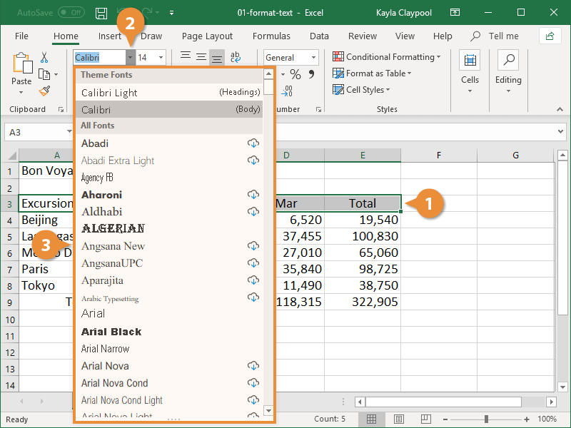
Change Fonts
Changing the font is a quick and simple way to enhance the appearance of your spreadsheet.
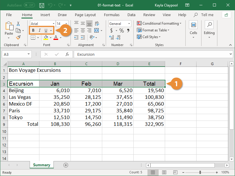
- Select the cells you want to format.
- Click the Font list arrow on the Home tab.
When text is selected in a cell, you can also click the Font list arrow on the Mini Toolbar.
- Select the font you want to use.

Apply Bold, Italic, or an Underline
In addition to changing the font type, you can amplify your project using other features in the Font group such as Bold, Italic, or Underline.
- Select the text you want to format.
- Click the Bold, Italic, or Underline buttons on the Home tab.
- To bold, press Ctrl + B.
- To italicize, press Ctrl + I.
- To underline, press Ctrl + U.
Click the Dialog Box Launcher in the Font group to see additional font formatting options. From the dialog box, you can change the underline style and add effects.
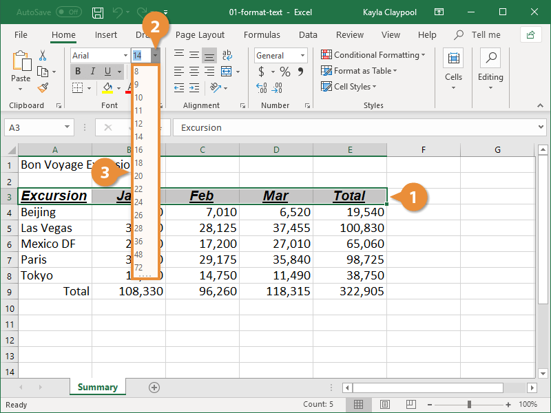
Change Font Size
Changing the font size can help differentiate between titles, headers, and body text.
- Select the cells you want to format.
- Click the Font Size list arrow.
Font size is measured in points (pt.) that are 1/72 of an inch. The larger the number of points, the larger the font.
- Select the font size you want.
Click the Increase Font Size or Decrease Font Size buttons on the Home tab to adjust the font size.
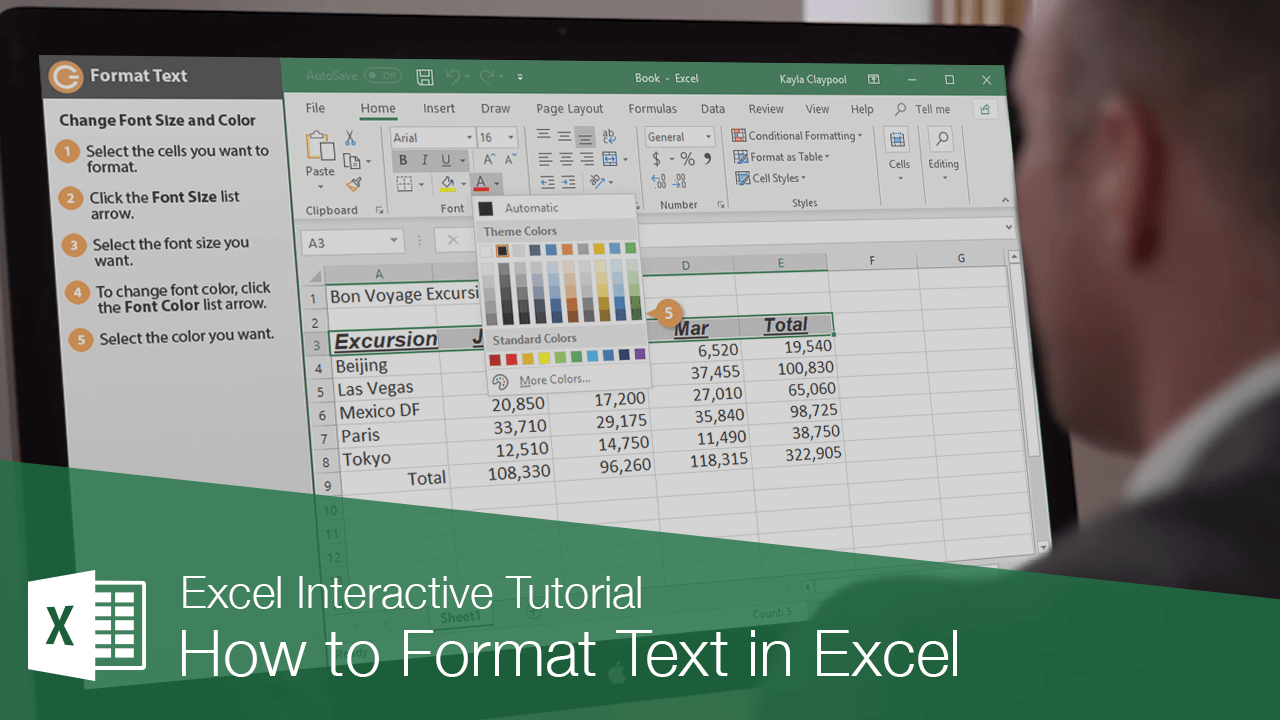
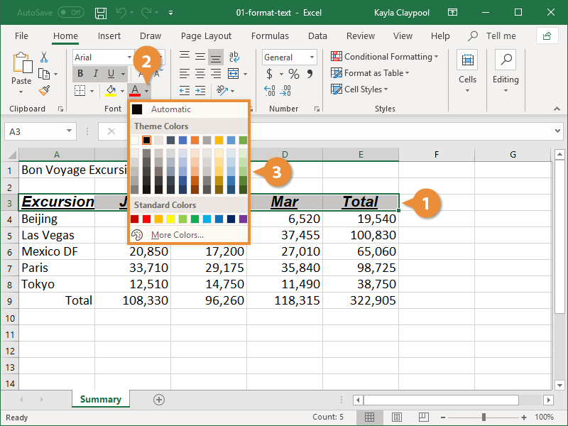
Change Font Color
Changing font color makes text stand out against the white background of the spreadsheet.
- Select the cells you want to format.
- Click the Font Color list arrow.
When text is selected in a cell, you can also click the Font Color list arrow on the Mini Toolbar.
- Select a new color.
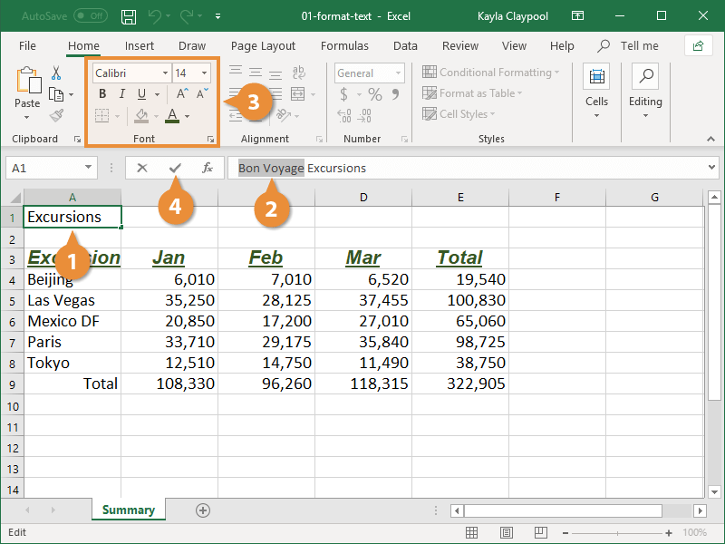
Format Part of a Cell
- Select the cell you want to format.
- In the formula bar, select the text you want to format.
- Select the text formatting you want to use.
- Press Enter.

FREE Quick Reference
Click to Download
Free to distribute with our compliments; we hope you will consider our paid training.
Formatting
Excel has many ways to format and style a spreadsheet.
Why format and style your spreadsheet?
- Make it easier to read and understand
- Make it more delicate
Styling is about changing the looks of cells, such as changing colors, font, font sizes, borders, number formats, and so on.
The most used styling functions are:
- Colors
- Fonts
- Borders
- Number formats
- Grids
There are two ways to access the styling commands in Excel:
- The Ribbon
- Formatting menu, by right clicking cells
Read more about the Ribbon in the Excel overview chapter.
Styling Commands in Ribbon

The Ribbon can be expanded by clicking the arrow/caret-down icon on the right side. This gives access to more commands:

Styling Commands, Right Clicking Cells
You can also right-click on any cell to style it:
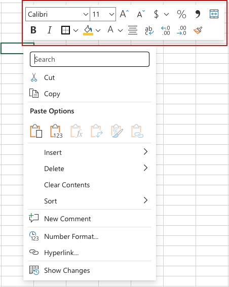
Styling commands can be accessed from both views.
Chapter summary
Formatting is used to make spreadsheets more readable. There are many ways to add styles. The most common ones are; Color, Font, Number format and Grids.
Formatting in Excel (2016, 2013 & 2010 and Others)
Formatting in Excel is a neat trick used to change the appearance of the data represented in the worksheet. We can do formatting in multiple ways, such as we can format the font of the cells or format the table by using the “Styles” and “Format” tabs available in the “Home” tab.
Table of contents
- Formatting in Excel (2016, 2013 & 2010 and Others)
- How to Format Data in Excel? (Step by Step)
- Shortcut Keys to Format Data in Excel
- Things to Remember
- Recommended Articles
How to Format Data in Excel? (Step by Step)
Let us understand the working of data formatting in Excel by simple examples. Now, suppose we have a simple report of sales for an organization as below:
You can download this Formatting Excel Template here – Formatting Excel Template

This report is not attractive to viewers. Therefore, we need to format the data.
Now, to format data in Excel, we must do the following:
- Bold the text of the column header.
- Make the font size larger.
- Adjust the column width using the shortcut key (Alt+H+O+I) after selecting the whole table (Ctrl+A).
- Align the data in the center.
- Apply the outline border by using (Alt+H+B+T)
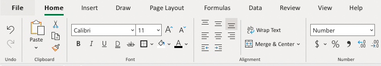
- Apply background color using the “Fill Color” command available in the “Font” group on the “Home” tab
We will be applying the same format for the table’s last “Total” row by using the “Format Painter” command available in the “Clipboard” group on the “Home” tab.

As the amount collected is a currency, we should format the same as “Currency” using the command available in the “Number” group placed on the “Home” tab.

After selecting the cells we need to format as currency, we need to open the “Format Cells” dialog box by clicking the above arrow.
Choose “Currency” and click on “OK.“

We can also apply the outline border to the table.

We will be creating the label for the report by using “Shapes.” To make the shape above the table, we need to add two new rows. So, we will select the row by “Shift+Spacebar” and then insert two rows by pressing “Ctrl+’+” twice.
We must choose an appropriate shape from the “Shapes” command available in the “Illustration” group in the “Insert” tab to insert the shape.

Create the shape according to the requirement and with the same color as the heads of the column. Then, add the text on the shape by right-clicking on the shapes and choosing “Edit Text.”

We can also use the “Format” contextual tab for formatting the shape using various commands such as “Shape Outline,” “Shape Fill,” “Text Fill,” “Text Outline,” etc. We can also apply the excel formatting on textText formatting in Excel include changing the colour, font name, font size, alignment, font appearance in bold, underlining, italic, background colour of the font cell, and so on.read more using the commands available in the “Font” group placed on the “Home” tab.


We can also use “Conditional Formatting” to take the viewers’ attention to the “Top 3” salesperson and “Bottom 3” salesperson.
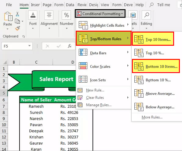
Format the cells that rank in the “Top 3” with “Green Fill with Dark Green Text.”

Also, format the cells that rank in the “Bottom 3” with “Light Red with Dark Red Text.”

We can also apply another conditional formatting option, “Data Bars.”

We can also create a chart to display the data, part of “Data Formatting Excel.”

Shortcut Keys to Format Data in Excel
- To make the text bold: Ctrl+B or Ctrl+2
- To make the text italic: Ctrl+I or Ctrl+3
- To make the text underline: Ctrl+U or Ctrl+4
- To make the font size of the text larger: Alt+H, FG
- To make the font size of the text smaller: Alt+H, FK
- To open the ”Font” dialog box: Alt+H,FN
- To open the ”Alignment” dialog box: Alt+H, FA
- To center align cell contents: Alt+H, A, then C
- To add borders: Alt+H, B
- To open the ”Format Cells” dialog box: Ctrl+1
- To apply or remove strikethrough data formatting Excel: Ctrl+5
- To apply an outline border to the selected cells: Ctrl+Shift+Ampersand(&)
- To apply the “Percentage” format with no decimal places: Ctrl+Shift+Percent (%)
- To add a non-adjacent cell or range to a selection of cells using the arrow keys: Shift+F8
Things to Remember
- While data formatting in Excel, we must make the title stand out, good and bold, it ensures it conveys the content we are showing. Next, we should enlarge the column and row heads and put them in a second color. Readers may quickly scan the column and row headings to get a sense of how the information on the worksheet is organized. This way, it can help them view what is most important on the page and where they should begin.
Recommended Articles
This article is a guide to Formatting in Excel. We discuss formatting data in Excel, Excel examples, and downloadable Excel templates here. You may also look at these useful functions in Excel: –
- Conditional Formatting in the Pivot Table
- Filters in Excel
- Examples of Data Table in Excel
- Gantt Chart in Excel