
Inserting rows and columns in Excel is very convenient when formatting tables and sheets. But function of inserting cells and entire adjacent and non-adjacent ranges enhances program features to new level.
Consider the practical examples how to add (or remove) cells and their ranges in the spreadsheet in Excel. In fact the cells are not added as the value moves on other. This fact should be taken into account when the sheet is filled with more than 50%. Then the remaining amount of cells for rows or columns may not be enough and this operation will delete the data. In such cases you should divide content of one sheet into 2 or 3 sheets. This is one of the main reasons why the new Excel version has more numbers of columns and rows (65,000 lines in the older versions and 1 000 000 in new one).
Inserting a range of empty cells
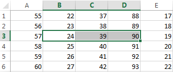
How to insert a cell in an Excel spreadsheet? Let’s say we have a table of values to which you want to insert two empty cells in between.
Perform the following procedure:
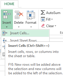
- Select the range in the place where you need to add new empty blocks. Go to the tab «HOME» — «Insert» — «Insert Cells». Or simply right click on the highlighted area and select the paste option. Or you may press the hotkey combination CTRL + SHIFT + «+».
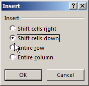
- A «Insert» dialog box appears where it is necessary to set the required parameters. In this case select «Shift down».
- Click OK. After that in the table with values new cells will be added. And the old will retain values and move down giving its place.
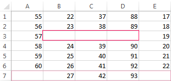
In this situation you can simply press the tool «HOME» — «Insert» (without choosing other options). Then the new cells will be inserted and the old ones will shift down (by default) without calling the dialog box options.
Use hotkeys combination CTRL + SHIFT + «plus» to add cells in Excel after selecting them.
Note. Pay attention to the settings dialog box. The last two parameters allow us to insert rows and columns in the same manner.
Removing cells
Now let’s remove the same range from our table with values. Just select the desired range. Right-click on the selected range and choose «Delete». Or go to the tab «HOME» — «Delete», «Shift up». The result is inversely proportional to the previous result.
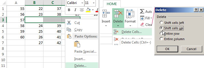
Select the range and use shortcut keys CTRL + «negative» if you want to remove cells in Excel.
Note. Likewise you can delete rows and columns.
Attention! In practice using tools «Insert» or «Delete» while inserting or deleting ranges without window with settings should be avoided so as not to get lost in the large and complex tables. Use the hotkeys if you want to save time. They cause a dialog box with removing the paste options and it also allows you to cope with the task much quickly.
In this Article
- Ranges and Cells in VBA
- Cell Address
- Range of Cells
- Writing to Cells
- Reading from Cells
- Non Contiguous Cells
- Intersection of Cells
- Offset from a Cell or Range
- Setting Reference to a Range
- Resize a Range
- OFFSET vs Resize
- All Cells in Sheet
- UsedRange
- CurrentRegion
- Range Properties
- Last Cell in Sheet
- Last Used Row Number in a Column
- Last Used Column Number in a Row
- Cell Properties
- Copy and Paste
- AutoFit Contents
- More Range Examples
- For Each
- Sort
- Find
- Range Address
- Range to Array
- Array to Range
- Sum Range
- Count Range
Ranges and Cells in VBA
Excel spreadsheets store data in Cells. Cells are arranged into Rows and Columns. Each cell can be identified by the intersection point of it’s row and column (Exs. B3 or R3C2).
An Excel Range refers to one or more cells (ex. A3:B4)
Cell Address
A1 Notation
In A1 notation, a cell is referred to by it’s column letter (from A to XFD) followed by it’s row number(from 1 to 1,048,576). This is called a cell address.
In VBA you can refer to any cell using the Range Object.
' Refer to cell B4 on the currently active sheet
MsgBox Range("B4")

' Refer to cell B4 on the sheet named 'Data'
MsgBox Worksheets("Data").Range("B4")

' Refer to cell B4 on the sheet named 'Data' in another OPEN workbook
' named 'My Data'
MsgBox Workbooks("My Data").Worksheets("Data").Range("B4")
R1C1 Notation
In R1C1 Notation a cell is referred by R followed by Row Number then letter ‘C’ followed by the Column Number. eg B4 in R1C1 notation will be referred by R4C2. In VBA you use the Cells Object to use R1C1 notation:
' Refer to cell R[6]C[4] i.e D6
Cells(6, 4) = "D6"
Range of Cells
A1 Notation
To refer to a more than one cell use a “:” between the starting cell address and last cell address. The following will refer to all the cells from A1 to D10:
Range("A1:D10")
R1C1 Notation
To refer to a more than one cell use a “,” between the starting cell address and last cell address. The following will refer to all the cells from A1 to D10:
Range(Cells(1, 1), Cells(10, 4))Writing to Cells
To write values to a cell or contiguous group of cells, simple refer to the range, put an = sign and then write the value to be stored:
' Store F5 in cell with Address F6
Range("F6") = "F6"

' Store E6 in cell with Address R[6]C[5] i.e E6
Cells(6, 5) = "E6"

' Store A1:D10 in the range A1:D10
Range("A1:D10") = "A1:D10"
' or
Range(Cells(1, 1), Cells(10, 4)) = "A1:D10"
Reading from Cells
To read values from cells, simple refer to the variable to store the values, put an = sign and then refer to the range to be read:
Dim val1
Dim val2

' Read from cell F6
val1 = Range("F6")

' Read from cell E6
val2 = Cells(6, 5)

MsgBox val1
Msgbox val2
Note: To store values from a range of cells, you need to use an Array instead of a simple variable.
Non Contiguous Cells
To refer to non contiguous cells use a comma between the cell addresses:
' Store 10 in cells A1, A3, and A5
Range("A1,A3,A5") = 10


' Store 10 in cells A1:A3 and D1:D3)
Range("A1:A3, D1:D3") = 10
VBA Coding Made Easy
Stop searching for VBA code online. Learn more about AutoMacro — A VBA Code Builder that allows beginners to code procedures from scratch with minimal coding knowledge and with many time-saving features for all users!

Learn More
Intersection of Cells
To refer to non contiguous cells use a space between the cell addresses:
' Store 'Col D' in D1:D10
' which is Common between A1:D10 and D1:F10
Range("A1:D10 D1:G10") = "Col D"
Offset from a Cell or Range
Using the Offset function, you can move the reference from a given Range (cell or group of cells) by the specified number_of_rows, and number_of_columns.
Offset Syntax
Range.Offset(number_of_rows, number_of_columns)
Offset from a cell
' OFFSET from a cell A1
' Refer to cell itself
' Move 0 rows and 0 columns
Range("A1").Offset(0, 0) = "A1"

' Move 1 rows and 0 columns
Range("A1").Offset(1, 0) = "A2"

' Move 0 rows and 1 columns
Range("A1").Offset(0, 1) = "B1"

' Move 1 rows and 1 columns
Range("A1").Offset(1, 1) = "B2"

' Move 10 rows and 5 columns
Range("A1").Offset(10, 5) = "F11"
Offset from a Range
' Move Reference to Range A1:D4 by 4 rows and 4 columns
' New Reference is E5:H8
Range("A1:D4").Offset(4,4) = "E5:H8"
Setting Reference to a Range
To assign a range to a range variable: declare a variable of type Range then use the Set command to set it to a range. Please note that you must use the SET command as RANGE is an object:
' Declare a Range variable
Dim myRange as Range

' Set the variable to the range A1:D4
Set myRange = Range("A1:D4")

' Prints $A$1:$D$4
MsgBox myRange.Address
VBA Programming | Code Generator does work for you!
Resize a Range
Resize method of Range object changes the dimension of the reference range:
Dim myRange As Range

' Range to Resize
Set myRange = Range("A1:F4")

' Prints $A$1:$E$10
Debug.Print myRange.Resize(10, 5).Address
Top-left cell of the Resized range is same as the top-left cell of the original range
Resize Syntax
Range.Resize(number_of_rows, number_of_columns)
OFFSET vs Resize
Offset does not change the dimensions of the range but moves it by the specified number of rows and columns. Resize does not change the position of the original range but changes the dimensions to the specified number of rows and columns.
All Cells in Sheet
The Cells object refers to all the cells in the sheet (1048576 rows and 16384 columns).
' Clear All Cells in Worksheets
Cells.Clear
UsedRange
UsedRange property gives you the rectangular range from the top-left cell used cell to the right-bottom used cell of the active sheet.
Dim ws As Worksheet
Set ws = ActiveSheet

' $B$2:$L$14 if L2 is the first cell with any value
' and L14 is the last cell with any value on the
' active sheet
Debug.Print ws.UsedRange.Address
CurrentRegion
CurrentRegion property gives you the contiguous rectangular range from the top-left cell to the right-bottom used cell containing the referenced cell/range.
Dim myRange As Range

Set myRange = Range("D4:F6")

' Prints $B$2:$L$14
' If there is a filled path from D4:F16 to B2 AND L14
Debug.Print myRange.CurrentRegion.Address

' You can refer to a single starting cell also

Set myRange = Range("D4") ' Prints $B$2:$L$14
AutoMacro | Ultimate VBA Add-in | Click for Free Trial!
Range Properties
You can get Address, row/column number of a cell, and number of rows/columns in a range as given below:
Dim myRange As Range

Set myRange = Range("A1:F10")

' Prints $A$1:$F$10
Debug.Print myRange.Address

Set myRange = Range("F10")

' Prints 10 for Row 10
Debug.Print myRange.Row

' Prints 6 for Column F
Debug.Print myRange.Column

Set myRange = Range("E1:F5")
' Prints 5 for number of Rows in range
Debug.Print myRange.Rows.Count

' Prints 2 for number of Columns in range
Debug.Print myRange.Columns.Count
Last Cell in Sheet
You can use Rows.Count and Columns.Count properties with Cells object to get the last cell on the sheet:
' Print the last row number
' Prints 1048576
Debug.Print "Rows in the sheet: " & Rows.Count

' Print the last column number
' Prints 16384
Debug.Print "Columns in the sheet: " & Columns.Count

' Print the address of the last cell
' Prints $XFD$1048576
Debug.Print "Address of Last Cell in the sheet: " & Cells(Rows.Count, Columns.Count)
Last Used Row Number in a Column
END property takes you the last cell in the range, and End(xlUp) takes you up to the first used cell from that cell.
Dim lastRow As Long

lastRow = Cells(Rows.Count, "A").End(xlUp).Row
Last Used Column Number in a Row
Dim lastCol As Long

lastCol = Cells(1, Columns.Count).End(xlToLeft).Column
END property takes you the last cell in the range, and End(xlToLeft) takes you left to the first used cell from that cell.
You can also use xlDown and xlToRight properties to navigate to the first bottom or right used cells of the current cell.
AutoMacro | Ultimate VBA Add-in | Click for Free Trial!
Cell Properties
Common Properties
Here is code to display commonly used Cell Properties
Dim cell As Range
Set cell = Range("A1")

cell.Activate
Debug.Print cell.Address
' Print $A$1

Debug.Print cell.Value
' Prints 456
' Address

Debug.Print cell.Formula
' Prints =SUM(C2:C3)

' Comment
Debug.Print cell.Comment.Text

' Style
Debug.Print cell.Style

' Cell Format
Debug.Print cell.DisplayFormat.NumberFormat
Cell Font
Cell.Font object contains properties of the Cell Font:
Dim cell As Range

Set cell = Range("A1")

' Regular, Italic, Bold, and Bold Italic
cell.Font.FontStyle = "Bold Italic"
' Same as
cell.Font.Bold = True
cell.Font.Italic = True

' Set font to Courier
cell.Font.FontStyle = "Courier"

' Set Font Color
cell.Font.Color = vbBlue
' or
cell.Font.Color = RGB(255, 0, 0)

' Set Font Size
cell.Font.Size = 20
Copy and Paste
Paste All
Ranges/Cells can be copied and pasted from one location to another. The following code copies all the properties of source range to destination range (equivalent to CTRL-C and CTRL-V)
'Simple Copy
Range("A1:D20").Copy
Worksheets("Sheet2").Range("B10").Paste

'or
' Copy from Current Sheet to sheet named 'Sheet2'
Range("A1:D20").Copy destination:=Worksheets("Sheet2").Range("B10")
Paste Special
Selected properties of the source range can be copied to the destination by using PASTESPECIAL option:
' Paste the range as Values only
Range("A1:D20").Copy
Worksheets("Sheet2").Range("B10").PasteSpecial Paste:=xlPasteValues
Here are the possible options for the Paste option:
' Paste Special Types
xlPasteAll
xlPasteAllExceptBorders
xlPasteAllMergingConditionalFormats
xlPasteAllUsingSourceTheme
xlPasteColumnWidths
xlPasteComments
xlPasteFormats
xlPasteFormulas
xlPasteFormulasAndNumberFormats
xlPasteValidation
xlPasteValues
xlPasteValuesAndNumberFormats
AutoFit Contents
Size of rows and columns can be changed to fit the contents using AutoFit:
' Change size of rows 1 to 5 to fit contents
Rows("1:5").AutoFit

' Change size of Columns A to B to fit contents
Columns("A:B").AutoFit
More Range Examples
It is recommended that you use Macro Recorder while performing the required action through the GUI. It will help you understand the various options available and how to use them.
AutoMacro | Ultimate VBA Add-in | Click for Free Trial!
For Each
It is easy to loop through a range using For Each construct as show below:
For Each cell In Range("A1:B100")
    ' Do something with the cell
Next cell
At each iteration of the loop one cell in the range is assigned to the variable cell and statements in the For loop are executed for that cell. Loop exits when all the cells are processed.
Sort
Sort is a method of Range object. You can sort a range by specifying options for sorting to Range.Sort. The code below will sort the columns A:C based on key in cell C2. Sort Order can be xlAscending or xlDescending. Header:= xlYes should be used if first row is the header row.
   Columns("A:C").Sort key1:=Range("C2"), _
      order1:=xlAscending, Header:=xlYes
Find
Find is also a method of Range Object. It find the first cell having content matching the search criteria and returns the cell as a Range object. It return Nothing if there is no match.
Use FindNext method (or FindPrevious) to find next(previous) occurrence.
Following code will change the font to “Arial Black” for all cells in the range which start with “John”:
For Each c In Range("A1:A100")
    If c Like "John*" Then
        c.Font.Name = "Arial Black"
    End If
Next c
Following code will replace all occurrences of “To Test” to “Passed” in the range specified:
With Range("a1:a500")
    Set c = .Find("To Test", LookIn:=xlValues)
    If Not c Is Nothing Then
        firstaddress = c.Address
        Do
            c.Value = "Passed"
            Set c = .FindNext(c)
        Loop While Not c Is Nothing And c.Address <> firstaddress
    End If
End With
It is important to note that you must specify a range to use FindNext. Also you must provide a stopping condition otherwise the loop will execute forever. Normally address of the first cell which is found is stored in a variable and loop is stopped when you reach that cell again. You must also check for the case when nothing is found to stop the loop.
Range Address
Use Range.Address to get the address in A1 Style
MsgBox Range("A1:D10").Address
' or
Debug.Print Range("A1:D10").Address
Use xlReferenceStyle (default is xlA1) to get addres in R1C1 style
MsgBox Range("A1:D10").Address(ReferenceStyle:=xlR1C1)
' or
Debug.Print Range("A1:D10").Address(ReferenceStyle:=xlR1C1)
This is useful when you deal with ranges stored in variables and want to process for certain addresses only.
AutoMacro | Ultimate VBA Add-in | Click for Free Trial!
Range to Array
It is faster and easier to transfer a range to an array and then process the values. You should declare the array as Variant to avoid calculating the size required to populate the range in the array. Array’s dimensions are set to match number of values in the range.
Dim DirArray As Variant
' Store the values in the range to the Array

DirArray = Range("a1:a5").Value

' Loop to process the values
For Each c In DirArray
    Debug.Print c
Next
Array to Range
After processing you can write the Array back to a Range. To write the Array in the example above to a Range you must specify a Range whose size matches the number of elements in the Array.
Use the code below to write the Array to the range D1:D5:
Range("D1:D5").Value = DirArray

Range("D1:H1").Value = Application.Transpose(DirArray)
Please note that you must Transpose the Array if you write it to a row.
Sum Range
SumOfRange = Application.WorksheetFunction.Sum(Range("A1:A10"))
Debug.Print SumOfRange
You can use many functions available in Excel in your VBA code by specifying Application.WorkSheetFunction. before the Function Name as in the example above.
Count Range
' Count Number of Cells with Numbers in the Range
CountOfCells = Application.WorksheetFunction.Count(Range("A1:A10"))
Debug.Print CountOfCells

' Count Number of Non Blank Cells in the Range
CountOfNonBlankCells = Application.WorksheetFunction.CountA(Range("A1:A10"))
Debug.Print CountOfNonBlankCells
Written by: Vinamra Chandra
I use this method in immediate mode when I don’t want to add code to the sheet.
strX="": _
For Each cllX in Range( ActiveCell, Cells( Cells.SpecialCells(xlCellTypeLastCell ).Row, ActiveCell.Column) ): _
strX=strX & iif(cllX.text="","",iif(strX="","",",")& cllX.address): _
Next: _
Range(strX).Select
But while that is intuitive, it only works for up to 35 to 50 cells. After that, the VBA returns an error 1004.
Run-time error '1004':
Application-defined or object-defined error
It is more robust to use the Union function.
Set rngX=ActiveCell: _
For Each cllX in Range( ActiveCell, Cells( cells.SpecialCells(xlCellTypeLastCell ).Row, ActiveCell.Column) ): _
Set rngX=iif( cllX.text="", rngX, Union(rngX, cllX) ): _
Next: _
rngX.Select
It is so short and intuitive, I just throw it away after each use.
“It is a capital mistake to theorize before one has data”- Sir Arthur Conan Doyle
This post covers everything you need to know about using Cells and Ranges in VBA. You can read it from start to finish as it is laid out in a logical order. If you prefer you can use the table of contents below to go to a section of your choice.
Topics covered include Offset property, reading values between cells, reading values to arrays and formatting cells.
A Quick Guide to Ranges and Cells
| Function | Takes | Returns | Example | Gives |
|---|---|---|---|---|
|
Range |
cell address | multiple cells | .Range(«A1:A4») | $A$1:$A$4 |
| Cells | row, column | one cell | .Cells(1,5) | $E$1 |
| Offset | row, column | multiple cells | Range(«A1:A2») .Offset(1,2) |
$C$2:$C$3 |
| Rows | row(s) | one or more rows | .Rows(4) .Rows(«2:4») |
$4:$4 $2:$4 |
| Columns | column(s) | one or more columns | .Columns(4) .Columns(«B:D») |
$D:$D $B:$D |
Download the Code
The Webinar
If you are a member of the VBA Vault, then click on the image below to access the webinar and the associated source code.
(Note: Website members have access to the full webinar archive.)

Introduction
This is the third post dealing with the three main elements of VBA. These three elements are the Workbooks, Worksheets and Ranges/Cells. Cells are by far the most important part of Excel. Almost everything you do in Excel starts and ends with Cells.
Generally speaking, you do three main things with Cells
- Read from a cell.
- Write to a cell.
- Change the format of a cell.
Excel has a number of methods for accessing cells such as Range, Cells and Offset.These can cause confusion as they do similar things and can lead to confusion
In this post I will tackle each one, explain why you need it and when you should use it.
Let’s start with the simplest method of accessing cells – using the Range property of the worksheet.
Important Notes
I have recently updated this article so that is uses Value2.
You may be wondering what is the difference between Value, Value2 and the default:
' Value2
Range("A1").Value2 = 56

' Value
Range("A1").Value = 56

' Default uses value
Range("A1") = 56
Using Value may truncate number if the cell is formatted as currency. If you don’t use any property then the default is Value.
It is better to use Value2 as it will always return the actual cell value(see this article from Charle Williams.)
The Range Property
The worksheet has a Range property which you can use to access cells in VBA. The Range property takes the same argument that most Excel Worksheet functions take e.g. “A1”, “A3:C6” etc.
The following example shows you how to place a value in a cell using the Range property.
' https://excelmacromastery.com/
Public Sub WriteToCell()

    ' Write number to cell A1 in sheet1 of this workbook
    ThisWorkbook.Worksheets("Sheet1").Range("A1").Value2 = 67

    ' Write text to cell A2 in sheet1 of this workbook
    ThisWorkbook.Worksheets("Sheet1").Range("A2").Value2 = "John Smith"

    ' Write date to cell A3 in sheet1 of this workbook
    ThisWorkbook.Worksheets("Sheet1").Range("A3").Value2 = #11/21/2017#

End Sub
As you can see Range is a member of the worksheet which in turn is a member of the Workbook. This follows the same hierarchy as in Excel so should be easy to understand. To do something with Range you must first specify the workbook and worksheet it belongs to.
For the rest of this post I will use the code name to reference the worksheet.

The following code shows the above example using the code name of the worksheet i.e. Sheet1 instead of ThisWorkbook.Worksheets(“Sheet1”).
' https://excelmacromastery.com/
Public Sub UsingCodeName()

    ' Write number to cell A1 in sheet1 of this workbook
    Sheet1.Range("A1").Value2 = 67

    ' Write text to cell A2 in sheet1 of this workbook
    Sheet1.Range("A2").Value2 = "John Smith"

    ' Write date to cell A3 in sheet1 of this workbook
    Sheet1.Range("A3").Value2 = #11/21/2017#

End Sub
You can also write to multiple cells using the Range property
' https://excelmacromastery.com/
Public Sub WriteToMulti()

    ' Write number to a range of cells
    Sheet1.Range("A1:A10").Value2 = 67

    ' Write text to multiple ranges of cells
    Sheet1.Range("B2:B5,B7:B9").Value2 = "John Smith"

End Sub
You can download working examples of all the code from this post from the top of this article.
The Cells Property of the Worksheet
The worksheet object has another property called Cells which is very similar to range. There are two differences
- Cells returns a range of one cell only.
- Cells takes row and column as arguments.
The example below shows you how to write values to cells using both the Range and Cells property
' https://excelmacromastery.com/
Public Sub UsingCells()

    ' Write to A1
    Sheet1.Range("A1").Value2 = 10
    Sheet1.Cells(1, 1).Value2  = 10

    ' Write to A10
    Sheet1.Range("A10").Value2 = 10
    Sheet1.Cells(10, 1).Value2  = 10

    ' Write to E1
    Sheet1.Range("E1").Value2 = 10
    Sheet1.Cells(1, 5).Value2  = 10

End Sub
You may be wondering when you should use Cells and when you should use Range. Using Range is useful for accessing the same cells each time the Macro runs.
For example, if you were using a Macro to calculate a total and write it to cell A10 every time then Range would be suitable for this task.
Using the Cells property is useful if you are accessing a cell based on a number that may vary. It is easier to explain this with an example.
In the following code, we ask the user to specify the column number. Using Cells gives us the flexibility to use a variable number for the column.
' https://excelmacromastery.com/
Public Sub WriteToColumn()

    Dim UserCol As Integer

    ' Get the column number from the user
    UserCol = Application.InputBox(" Please enter the column...", Type:=1)

    ' Write text to user selected column
    Sheet1.Cells(1, UserCol).Value2 = "John Smith"

End Sub
In the above example, we are using a number for the column rather than a letter.
To use Range here would require us to convert these values to the letter/number cell reference e.g. “C1”. Using the Cells property allows us to provide a row and a column number to access a cell.
Sometimes you may want to return more than one cell using row and column numbers. The next section shows you how to do this.
Using Cells and Range together
As you have seen you can only access one cell using the Cells property. If you want to return a range of cells then you can use Cells with Ranges as follows
' https://excelmacromastery.com/
Public Sub UsingCellsWithRange()

    With Sheet1
        ' Write 5 to Range A1:A10 using Cells property
        .Range(.Cells(1, 1), .Cells(10, 1)).Value2 = 5

        ' Format Range B1:Z1 to be bold
        .Range(.Cells(1, 2), .Cells(1, 26)).Font.Bold = True

    End With

End Sub
As you can see, you provide the start and end cell of the Range. Sometimes it can be tricky to see which range you are dealing with when the value are all numbers. Range has a property called Address which displays the letter/ number cell reference of any range. This can come in very handy when you are debugging or writing code for the first time.
In the following example we print out the address of the ranges we are using:
' https://excelmacromastery.com/
Public Sub ShowRangeAddress()

    ' Note: Using underscore allows you to split up lines of code
    With Sheet1

        ' Write 5 to Range A1:A10 using Cells property
        .Range(.Cells(1, 1), .Cells(10, 1)).Value2 = 5
        Debug.Print "First address is : " _
            + .Range(.Cells(1, 1), .Cells(10, 1)).Address

        ' Format Range B1:Z1 to be bold
        .Range(.Cells(1, 2), .Cells(1, 26)).Font.Bold = True
        Debug.Print "Second address is : " _
            + .Range(.Cells(1, 2), .Cells(1, 26)).Address

    End With

End Sub
In the example I used Debug.Print to print to the Immediate Window. To view this window select View->Immediate Window(or Ctrl G)


You can download all the code for this post from the top of this article.
The Offset Property of Range
Range has a property called Offset. The term Offset refers to a count from the original position. It is used a lot in certain areas of programming. With the Offset property you can get a Range of cells the same size and a certain distance from the current range. The reason this is useful is that sometimes you may want to select a Range based on a certain condition. For example in the screenshot below there is a column for each day of the week. Given the day number(i.e. Monday=1, Tuesday=2 etc.) we need to write the value to the correct column.

We will first attempt to do this without using Offset.
' https://excelmacromastery.com/
' This sub tests with different values
Public Sub TestSelect()

    ' Monday
    SetValueSelect 1, 111.21
    ' Wednesday
    SetValueSelect 3, 456.99
    ' Friday
    SetValueSelect 5, 432.25
    ' Sunday
    SetValueSelect 7, 710.17

End Sub

' Writes the value to a column based on the day
Public Sub SetValueSelect(lDay As Long, lValue As Currency)

    Select Case lDay
        Case 1: Sheet1.Range("H3").Value2 = lValue
        Case 2: Sheet1.Range("I3").Value2 = lValue
        Case 3: Sheet1.Range("J3").Value2 = lValue
        Case 4: Sheet1.Range("K3").Value2 = lValue
        Case 5: Sheet1.Range("L3").Value2 = lValue
        Case 6: Sheet1.Range("M3").Value2 = lValue
        Case 7: Sheet1.Range("N3").Value2 = lValue
    End Select

End Sub
As you can see in the example, we need to add a line for each possible option. This is not an ideal situation. Using the Offset Property provides a much cleaner solution
' https://excelmacromastery.com/
' This sub tests with different values
Public Sub TestOffset()

    DayOffSet 1, 111.01
    DayOffSet 3, 456.99
    DayOffSet 5, 432.25
    DayOffSet 7, 710.17

End Sub

Public Sub DayOffSet(lDay As Long, lValue As Currency)

    ' We use the day value with offset specify the correct column
    Sheet1.Range("G3").Offset(, lDay).Value2 = lValue

End Sub
As you can see this solution is much better. If the number of days in increased then we do not need to add any more code. For Offset to be useful there needs to be some kind of relationship between the positions of the cells. If the Day columns in the above example were random then we could not use Offset. We would have to use the first solution.
One thing to keep in mind is that Offset retains the size of the range. So .Range(“A1:A3”).Offset(1,1) returns the range B2:B4. Below are some more examples of using Offset
' https://excelmacromastery.com/
Public Sub UsingOffset()

    ' Write to B2 - no offset
    Sheet1.Range("B2").Offset().Value2 = "Cell B2"

    ' Write to C2 - 1 column to the right
    Sheet1.Range("B2").Offset(, 1).Value2 = "Cell C2"

    ' Write to B3 - 1 row down
    Sheet1.Range("B2").Offset(1).Value2 = "Cell B3"

    ' Write to C3 - 1 column right and 1 row down
    Sheet1.Range("B2").Offset(1, 1).Value2 = "Cell C3"

    ' Write to A1 - 1 column left and 1 row up
    Sheet1.Range("B2").Offset(-1, -1).Value2 = "Cell A1"

    ' Write to range E3:G13 - 1 column right and 1 row down
    Sheet1.Range("D2:F12").Offset(1, 1).Value2 = "Cells E3:G13"

End Sub
Using the Range CurrentRegion
CurrentRegion returns a range of all the adjacent cells to the given range.
In the screenshot below you can see the two current regions. I have added borders to make the current regions clear.

A row or column of blank cells signifies the end of a current region.
You can manually check the CurrentRegion in Excel by selecting a range and pressing Ctrl + Shift + *.
If we take any range of cells within the border and apply CurrentRegion, we will get back the range of cells in the entire area.
For example
Range(“B3”).CurrentRegion will return the range B3:D14
Range(“D14”).CurrentRegion will return the range B3:D14
Range(“C8:C9”).CurrentRegion will return the range B3:D14
and so on
How to Use
We get the CurrentRegion as follows
' Current region will return B3:D14 from above example
Dim rg As Range
Set rg = Sheet1.Range("B3").CurrentRegion
Read Data Rows Only
Read through the range from the second row i.e.skipping the header row
' Current region will return B3:D14 from above example
Dim rg As Range
Set rg = Sheet1.Range("B3").CurrentRegion

' Start at row 2 - row after header
Dim i As Long
For i = 2 To rg.Rows.Count
    ' current row, column 1 of range
    Debug.Print rg.Cells(i, 1).Value2
Next i
Remove Header
Remove header row(i.e. first row) from the range. For example if range is A1:D4 this will return A2:D4
' Current region will return B3:D14 from above example
Dim rg As Range
Set rg = Sheet1.Range("B3").CurrentRegion

' Remove Header
Set rg = rg.Resize(rg.Rows.Count - 1).Offset(1)

' Start at row 1 as no header row
Dim i As Long
For i = 1 To rg.Rows.Count
    ' current row, column 1 of range
    Debug.Print rg.Cells(i, 1).Value2
Next i
Using Rows and Columns as Ranges
If you want to do something with an entire Row or Column you can use the Rows or Columns property of the Worksheet. They both take one parameter which is the row or column number you wish to access
' https://excelmacromastery.com/
Public Sub UseRowAndColumns()

    ' Set the font size of column B to 9
    Sheet1.Columns(2).Font.Size = 9

    ' Set the width of columns D to F
    Sheet1.Columns("D:F").ColumnWidth = 4

    ' Set the font size of row 5 to 18
    Sheet1.Rows(5).Font.Size = 18

End Sub
Using Range in place of Worksheet
You can also use Cells, Rows and Columns as part of a Range rather than part of a Worksheet. You may have a specific need to do this but otherwise I would avoid the practice. It makes the code more complex. Simple code is your friend. It reduces the possibility of errors.
The code below will set the second column of the range to bold. As the range has only two rows the entire column is considered B1:B2
' https://excelmacromastery.com/
Public Sub UseColumnsInRange()

    ' This will set B1 and B2 to be bold
    Sheet1.Range("A1:C2").Columns(2).Font.Bold = True

End Sub
You can download all the code for this post from the top of this article.
Reading Values from one Cell to another
In most of the examples so far we have written values to a cell. We do this by placing the range on the left of the equals sign and the value to place in the cell on the right. To write data from one cell to another we do the same. The destination range goes on the left and the source range goes on the right.
The following example shows you how to do this:
' https://excelmacromastery.com/
Public Sub ReadValues()

    ' Place value from B1 in A1
    Sheet1.Range("A1").Value2 = Sheet1.Range("B1").Value2

    ' Place value from B3 in sheet2 to cell A1
    Sheet1.Range("A1").Value2 = Sheet2.Range("B3").Value2

    ' Place value from B1 in cells A1 to A5
    Sheet1.Range("A1:A5").Value2 = Sheet1.Range("B1").Value2

    ' You need to use the "Value" property to read multiple cells
    Sheet1.Range("A1:A5").Value2 = Sheet1.Range("B1:B5").Value2

End Sub
As you can see from this example it is not possible to read from multiple cells. If you want to do this you can use the Copy function of Range with the Destination parameter
' https://excelmacromastery.com/
Public Sub CopyValues()

    ' Store the copy range in a variable
    Dim rgCopy As Range
    Set rgCopy = Sheet1.Range("B1:B5")

    ' Use this to copy from more than one cell
    rgCopy.Copy Destination:=Sheet1.Range("A1:A5")

    ' You can paste to multiple destinations
    rgCopy.Copy Destination:=Sheet1.Range("A1:A5,C2:C6")

End Sub
The Copy function copies everything including the format of the cells. It is the same result as manually copying and pasting a selection. You can see more about it in the Copying and Pasting Cells section.
Using the Range.Resize Method
When copying from one range to another using assignment(i.e. the equals sign), the destination range must be the same size as the source range.
Using the Resize function allows us to resize a range to a given number of rows and columns.
For example:
' https://excelmacromastery.com/
Sub ResizeExamples()

    ' Prints A1
    Debug.Print Sheet1.Range("A1").Address

    ' Prints A1:A2
    Debug.Print Sheet1.Range("A1").Resize(2, 1).Address

    ' Prints A1:A5
    Debug.Print Sheet1.Range("A1").Resize(5, 1).Address

    ' Prints A1:D1
    Debug.Print Sheet1.Range("A1").Resize(1, 4).Address

    ' Prints A1:C3
    Debug.Print Sheet1.Range("A1").Resize(3, 3).Address

End Sub
When we want to resize our destination range we can simply use the source range size.
In other words, we use the row and column count of the source range as the parameters for resizing:
' https://excelmacromastery.com/
Sub Resize()

    Dim rgSrc As Range, rgDest As Range

    ' Get all the data in the current region
    Set rgSrc = Sheet1.Range("A1").CurrentRegion

      ' Get the range destination
    Set rgDest = Sheet2.Range("A1")
    Set rgDest = rgDest.Resize(rgSrc.Rows.Count, rgSrc.Columns.Count)

    rgDest.Value2 = rgSrc.Value2

End Sub
We can do the resize in one line if we prefer:
' https://excelmacromastery.com/
Sub ResizeOneLine()

    Dim rgSrc As Range

    ' Get all the data in the current region
    Set rgSrc = Sheet1.Range("A1").CurrentRegion

    With rgSrc
        Sheet2.Range("A1").Resize(.Rows.Count, .Columns.Count).Value2 = .Value2
    End With

End Sub
Reading Values to variables
We looked at how to read from one cell to another. You can also read from a cell to a variable. A variable is used to store values while a Macro is running. You normally do this when you want to manipulate the data before writing it somewhere. The following is a simple example using a variable. As you can see the value of the item to the right of the equals is written to the item to the left of the equals.
' https://excelmacromastery.com/
Public Sub UseVariables()

    ' Create
    Dim number As Long

    ' Read number from cell
    number = Sheet1.Range("A1").Value2

    ' Add 1 to value
    number = number + 1

    ' Write new value to cell
    Sheet1.Range("A2").Value2 = number

End Sub
To read text to a variable you use a variable of type String:
' https://excelmacromastery.com/
Public Sub UseVariableText()

    ' Declare a variable of type string
    Dim text As String

    ' Read value from cell
    text = Sheet1.Range("A1").Value2

    ' Write value to cell
    Sheet1.Range("A2").Value2 = text

End Sub
You can write a variable to a range of cells. You just specify the range on the left and the value will be written to all cells in the range.
' https://excelmacromastery.com/
Public Sub VarToMulti()

    ' Read value from cell
    Sheet1.Range("A1:B10").Value2 = 66

End Sub
You cannot read from multiple cells to a variable. However you can read to an array which is a collection of variables. We will look at doing this in the next section.
How to Copy and Paste Cells
If you want to copy and paste a range of cells then you do not need to select them. This is a common error made by new VBA users.
Note: We normally use Range.Copy when we want to copy formats, formulas, validation. If we want to copy values it is not the most efficient method.
I have written a complete guide to copying data in Excel VBA here.
You can simply copy a range of cells like this:
Range("A1:B4").Copy Destination:=Range("C5")
Using this method copies everything – values, formats, formulas and so on. If you want to copy individual items you can use the PasteSpecial property of range.
It works like this
Range("A1:B4").Copy
Range("F3").PasteSpecial Paste:=xlPasteValues
Range("F3").PasteSpecial Paste:=xlPasteFormats
Range("F3").PasteSpecial Paste:=xlPasteFormulas
The following table shows a full list of all the paste types
| Paste Type |
|---|
| xlPasteAll |
| xlPasteAllExceptBorders |
| xlPasteAllMergingConditionalFormats |
| xlPasteAllUsingSourceTheme |
| xlPasteColumnWidths |
| xlPasteComments |
| xlPasteFormats |
| xlPasteFormulas |
| xlPasteFormulasAndNumberFormats |
| xlPasteValidation |
| xlPasteValues |
| xlPasteValuesAndNumberFormats |
Reading a Range of Cells to an Array
You can also copy values by assigning the value of one range to another.
Range("A3:Z3").Value2 = Range("A1:Z1").Value2
The value of range in this example is considered to be a variant array. What this means is that you can easily read from a range of cells to an array. You can also write from an array to a range of cells. If you are not familiar with arrays you can check them out in this post.
The following code shows an example of using an array with a range:
' https://excelmacromastery.com/
Public Sub ReadToArray()

    ' Create dynamic array
    Dim StudentMarks() As Variant

    ' Read 26 values into array from the first row
    StudentMarks = Range("A1:Z1").Value2

    ' Do something with array here

    ' Write the 26 values to the third row
    Range("A3:Z3").Value2 = StudentMarks

End Sub
Keep in mind that the array created by the read is a 2 dimensional array. This is because a spreadsheet stores values in two dimensions i.e. rows and columns
Going through all the cells in a Range
Sometimes you may want to go through each cell one at a time to check value.
You can do this using a For Each loop shown in the following code
' https://excelmacromastery.com/
Public Sub TraversingCells()

    ' Go through each cells in the range
    Dim rg As Range
    For Each rg In Sheet1.Range("A1:A10,A20")
        ' Print address of cells that are negative
        If rg.Value < 0 Then
            Debug.Print rg.Address + " is negative."
        End If
    Next

End Sub
You can also go through consecutive Cells using the Cells property and a standard For loop.
The standard loop is more flexible about the order you use but it is slower than a For Each loop.
' https://excelmacromastery.com/
Public Sub TraverseCells()

    ' Go through cells from A1 to A10
    Dim i As Long
    For i = 1 To 10
        ' Print address of cells that are negative
        If Range("A" & i).Value < 0 Then
            Debug.Print Range("A" & i).Address + " is negative."
        End If
    Next

    ' Go through cells in reverse i.e. from A10 to A1
    For i = 10 To 1 Step -1
        ' Print address of cells that are negative
        If Range("A" & i) < 0 Then
            Debug.Print Range("A" & i).Address + " is negative."
        End If
    Next

End Sub
Formatting Cells
Sometimes you will need to format the cells the in spreadsheet. This is actually very straightforward. The following example shows you various formatting you can add to any range of cells
' https://excelmacromastery.com/
Public Sub FormattingCells()

    With Sheet1

        ' Format the font
        .Range("A1").Font.Bold = True
        .Range("A1").Font.Underline = True
        .Range("A1").Font.Color = rgbNavy

        ' Set the number format to 2 decimal places
        .Range("B2").NumberFormat = "0.00"
        ' Set the number format to a date
        .Range("C2").NumberFormat = "dd/mm/yyyy"
        ' Set the number format to general
        .Range("C3").NumberFormat = "General"
        ' Set the number format to text
        .Range("C4").NumberFormat = "Text"

        ' Set the fill color of the cell
        .Range("B3").Interior.Color = rgbSandyBrown

        ' Format the borders
        .Range("B4").Borders.LineStyle = xlDash
        .Range("B4").Borders.Color = rgbBlueViolet

    End With

End Sub
Main Points
The following is a summary of the main points
- Range returns a range of cells
- Cells returns one cells only
- You can read from one cell to another
- You can read from a range of cells to another range of cells.
- You can read values from cells to variables and vice versa.
- You can read values from ranges to arrays and vice versa
- You can use a For Each or For loop to run through every cell in a range.
- The properties Rows and Columns allow you to access a range of cells of these types
What’s Next?
Free VBA Tutorial If you are new to VBA or you want to sharpen your existing VBA skills then why not try out the The Ultimate VBA Tutorial.
Related Training: Get full access to the Excel VBA training webinars and all the tutorials.
(NOTE: Planning to build or manage a VBA Application? Learn how to build 10 Excel VBA applications from scratch.)
Introduction to Range and Cells in VBA
When you look around in an Excel workbook, you will find that everything works around cells. A cell and a range of cells are where you store your data, and then everything starts.
To make the best of VBA, you need to learn how to use cells and ranges in your codes. For this, you need to have a solid understanding of Range objects. By using it, you can refer to cells in your codes in the following ways:
- A single cell.
- A range of cells
- A row or a column
- A three-dimensional range
The RANGE OBJECT is a part of Excel’s Object Hierarchy: Application ➜ Workbooks ➜ Worksheets ➜ Range and besides inside the worksheet. So if you are writing code to refer to the RANGE object it would be like this:
Application.Workbook(“Workbook-Name”).Worksheets(“Sheet-Name”).RangeBy referring to a cell or range of cells, you can do the following things:
- You can read the value from it.
- You can enter a value in it.
- And, you can make changes to the format.
To do all these things, you need to learn to refer to a cell or a range of cells, and in the next section of this tutorial, you will learn to refer to a cell using different ways.
To refer to a cell or a range of cells, you can use three different ways.
- Range Property
- Cells Property
- Offset Property
Well, which one is best out of these depends on your requirement, but it is worth learning all three so that you can choose which one is perfect for you.
So let’s get started.
Range Property
Range property is the most common and popular way to refer to a range in your VBA codes. With Range property, you simply need to refer to the cell address. Let me tell you the syntax.
expression.range(address)Here the expression is a variable representing a VBA object. So if you need to refer to the cell A1, the line of code you need to write would be:
Application.Workbook(“Book1”).Worksheets(“Sheet1”).Range(“A1”)The above code tells VBA that you are referring to cell A1 which is in the worksheet “Sheet1” and workbook ”Book1”.
Note: Whenever you type a cell address in the range object, make sure to wrap it in double quotation marks. But here’s one thing to understand. As you are using VBA in Excel there’s no need to use the word “Application”. So the code would be:
Workbook(“Book1”).Worksheets(“Sheet1”).Range(“A1”)And if you are in the Book1 there you can further trim down your code:
Worksheets(“Sheet1”).Range(“A1”)But, if you are already in the worksheet “Sheet1” then you can further trim down your code and can only use:
Range(“A1”)Now, let’s say if you want to refer to a full range of cells (i.e., multiple cells) you need to write the code in the following way:
Range("A1:A5")In the above code, you have referred to the range A1 to A5 which consists of the five cells. You can also refer to a named range using the range object. Let’s say you have named range with the name of “Sales Discount” to refer to this you can write a code like this:
Range("Sales Discount")If you want to refer to a non-continues range then you need to do something like this:
Range("A1:B5,D5:G10")And if you want to refer to an entire row or a column then you need to enter code like the below:
Range("1:1")
Range("A:A")
At this point, you have a clear understanding of how to refer to a cell and the range of cells. But to make it best with this you need to learn how to use this to do other things.
here we have a complete list of tutorials that you can use to learn to work with ranges and cells in VBA
- How to SET (Get and Change) Cell Value using a VBA Code
- How to Select a Range using VBA in Excel
- How to Create a Named Range using VBA (Static + Dynamic) in Excel
- How to Merge and Unmerge Cells in Excel using a VBA Code
- How to Check IF a Cell is Empty using VBA in Excel
- VBA ClearContents (from a Cell, Range, or Entire Worksheet)
- Excel VBA Font (Color, Size, Type, and Bold)
- How to AutoFit (Rows, Column, or the Entire Worksheet) using VBA
- How to use OFFSET Property with the Range Object or a Cell in VBA
- VBA Wrap Text (Cell, Range, and Entire Worksheet)
- How to Copy a CellRange to Another Sheet using VBA
- How to use Range/Cell as a Variable in VBA in Excel
- How to Find Last Rows, Column, and Cell using VBA in Excel
- How to use ActiveCell in VBA in Excel
- How to Refer to the UsedRange using VBA in Excel
- How to Change Row Height/Column Width using VBA in Excel
- How to SELECT ALL the Cells in a Worksheet using a VBA Code
- How to Insert a Row using VBA in Excel
- How to Insert a Column using VBA in Excel
1. Select and Activate a Cell
If you want to select a cell then you can use the Range. Select method. Let’s say if you want to select cell A5 then all you need to do is specify the range and then add “.Select” after that.
Range(“A1”).SelectThis code tells VBA to select cell A5 and if you want to select a range of cells then you just need to refer to that range and simply add “.Select” after that.
Range(“A1:A5”).SelectThere’s also another method that you can use to activate a cell.
Range(“A1”).ActivateHere you need to remember that you can activate only one cell at a time. Even if you specify a range with the “.Activate” method, it will select that range but the active cell will be the first cell of the range.
2. Enter a Value in a Cell
By using the range property you can enter a value in a cell or a range of cells. Let’s understand how it works using a simple example:
Range("A1").Value = "ExcelChamps"In the above example, you have specified the A1 as a range and after that, you have added “.Value” which tells VBA to access the value property of the cell.
The next thing you have is the equals sign and then the value which you want to enter (you need to use double quotation marks if you are entering a text value). For a number, the code would like this:
Range("A1").Value = 9988And if you want to enter a value into a range of cells, I mean multiple cells, then all you need to do is specify that range.
Range("A1:A5").Value = "ExcelChamps"And, here’s the code if you are referring to the non-continues range.
Range("A1:A5 , E2:E3").Value = "ExcelChamps"3. Copy and Paste a Cell/Range
With Range property, you can use the “.Copy” method to copy and cell and then paste it into a destination cell. Let’s say if you need to copy the cell A5 the code for this would be:
Range("A5").Copy When you run this code it will simply copy cell A5 but the next thing is to paste this copied cell to a destination cell. For this, you need to add the keyword destination after it and followed by the cell where you want to paste it. So if you want to copy cell A1 and then want to paste it to the cell E5, the code would be:
Range("A1").Copy Destination:=Range("E5")In the same way, if you are dealing with a range of multiple cells then the code would be like:
Range("A1:A5").Copy Destination:=Range("E5:E9")If you have copied a range of cells and then if you have mentioned one cell as the destination range, VBA will copy the entire copied range the starting from the cell you have specified as a destination.
Range("A1:A5").Copy Destination:=Range("B1")When you run the above code, VBA will copy range A1:A5 and will paste it to the B1:B5 even though you have mentioned only B1 as the destination range.
Tip: Just like the “.Copy” method you can use the “.Cut” method to cut a cell and then simply use a destination to paste it.
4. Use Font Property with Range Property
With the range property, you can access the font property of a cell which helps you to change all the font settings. There are a total of 18 different properties for the font which you can access. Let’s say if you want to make the text BOLD in cell A1, the code would be:
Range("A1").Font.Bold = TrueThis code tells VBA to access the BOLD property of the font which is inside the range A1 and you have set this property to TRUE. Now, let’s say you want to apply strikethrough to cell A1, this time the code would be:
As I said there are a total of 18 different properties you can use, so make sure to check out all of these to see which one is useful for you.
5. Clear Formatting from a Cell
By using the “.ClearFormats” method you can remove only the format from a cell or a range of cells. All you need to do is add “.ClearFormat” after specifying the range, like below:
Range("A1").ClearFormatsWhen you run the code above it clears all the formatting from cell A1 and if you want to do it for an entire range, you know what to do, Right?
Range("A1:A5").ClearFormatsNow the above code will simply remove the formatting from the range A1 to A5.
Cells Property
Apart from the RANGE property, you can use the “Cells” property to refer to a cell or a range of cells in your worksheet. In cell property, instead of using the cell reference, you need to enter the column number and row number of the cell.
expression.Cells(Row_Number, Column_Number)Here the expression is a VBA object and Row_Number is the row number of the cell and Column_Number is the column of the cell. So if you want to refer to the cell A5 you can use the code below code:
Cells(5,1)Now, this code tells VBA to refer to the cell which is at row number five and at column number one. As its syntax says you need to enter column number as address but the reality is you can also use the column alphabet if you want just by wrapping it in double quotation marks.
The below code will also refer to the cell A5:
Cells(5,"A")And to VBA to select it simply add “.Select” at the end.
Cells(5,1).SelectThe above code will select cell A5 which is in the 5th row and in the first column of the worksheet.
OFFSET Property
If you want to play well with ranges in VBA you need to know how to use the OFFSET property. It helps to refer to a cell that is a particular number of rows and columns away from another cell.
Let’s say your active cell is B5 right now and you want to navigate to the cell which is 3 columns right and 1 row down from B5, you can do this OFFSET. Below is the syntax which you need to use for the OFFSET:
expression.Offset (RowOffset, ColumnOffset)- RowOffset: In this argument, you need to specify a number that will tell VBA how many rows you want to navigate. A positive number defines a row downward and a negative number defines a row upward.
- ColumnOffset: In this argument, you need to specify a number that will tell VBA how many columns you want to navigate. A positive number defines a column to the right and a negative number defines a left.
Let’s write a simple code for example which we have discussed above.
- First, you need to define the range from where you want to navigate and so type the below code:

- After that, type “.Offset” and enter opening parentheses, just like below:

- Next, you need to enter the row number and then the column number where you want to navigate.

- In the end, you need to add “.Select” to tell VBA to select the cell where you want to navigate.


So when you run this code it will select the cell which is one row down and 3 columns right from cell B5.
Resize a Range using OFFSET
OFFSET not only allows you to navigate to a cell, but you can also resize the range further. Let’s continue the above example.
Range("B5").Offset(1, 3).SelectThe above code navigates you to cell E6, and now let’s say you need to select the range of cells that consists of the five columns and three rows from the E6. So what you need to do is after using OFFSET, use the resize property by adding “.Resize”.
Range("B5").Offset(1, 3).ResizeNow you need to enter the row size and column size. Type a starting parenthesis and enter the number to define the row size and then a number to define the column size.
Range("B5").Offset(1, 3).Resize(3,5)In the end, add “.Select” to tell VBA to select the range, and when you run this code, it will select the range.
Range("B5").Offset(1, 3).Resize(3, 5).SelectSo, when you run this code, it will select the range E6 to I8.
Range("A1").Font.Strikethrough = TrueMore Tutorials
- Count Rows using VBA in Excel
- Excel VBA Font (Color, Size, Type, and Bold)
- Excel VBA Hide and Unhide a Column or a Row
- Apply Borders on a Cell using VBA in Excel
- Find Last Row, Column, and Cell using VBA in Excel
- Insert a Row using VBA in Excel
- Merge Cells in Excel using a VBA Code
- Select a Range/Cell using VBA in Excel
- SELECT ALL the Cells in a Worksheet using a VBA Code
- ActiveCell in VBA in Excel
- Special Cells Method in VBA in Excel
- UsedRange Property in VBA in Excel
- VBA AutoFit (Rows, Column, or the Entire Worksheet)
- VBA ClearContents (from a Cell, Range, or Entire Worksheet)
- VBA Copy Range to Another Sheet + Workbook
- VBA Enter Value in a Cell (Set, Get and Change)
- VBA Insert Column (Single and Multiple)
- VBA Named Range | (Static + from Selection + Dynamic)
- VBA Range Offset
- VBA Sort Range | (Descending, Multiple Columns, Sort Orientation
- VBA Wrap Text (Cell, Range, and Entire Worksheet)
- VBA Check IF a Cell is Empty + Multiple Cells
⇠ Back to What is VBA in Excel
Helpful Links – Developer Tab – Visual Basic Editor – Run a Macro – Personal Macro Workbook – Excel Macro Recorder – VBA Interview Questions – VBA Codes
На чтение 18 мин. Просмотров 74.5k.

сэр Артур Конан Дойл
Это большая ошибка — теоретизировать, прежде чем кто-то получит данные
Эта статья охватывает все, что вам нужно знать об использовании ячеек и диапазонов в VBA. Вы можете прочитать его от начала до конца, так как он сложен в логическом порядке. Или использовать оглавление ниже, чтобы перейти к разделу по вашему выбору.
Рассматриваемые темы включают свойство смещения, чтение
значений между ячейками, чтение значений в массивы и форматирование ячеек.
Содержание
- Краткое руководство по диапазонам и клеткам
- Введение
- Важное замечание
- Свойство Range
- Свойство Cells рабочего листа
- Использование Cells и Range вместе
- Свойство Offset диапазона
- Использование диапазона CurrentRegion
- Использование Rows и Columns в качестве Ranges
- Использование Range вместо Worksheet
- Чтение значений из одной ячейки в другую
- Использование метода Range.Resize
- Чтение Value в переменные
- Как копировать и вставлять ячейки
- Чтение диапазона ячеек в массив
- Пройти через все клетки в диапазоне
- Форматирование ячеек
- Основные моменты
Краткое руководство по диапазонам и клеткам
| Функция | Принимает | Возвращает | Пример | Вид |
| Range | адреса ячеек |
диапазон ячеек |
.Range(«A1:A4») | $A$1:$A$4 |
| Cells | строка, столбец |
одна ячейка |
.Cells(1,5) | $E$1 |
| Offset | строка, столбец |
диапазон | .Range(«A1:A2») .Offset(1,2) |
$C$2:$C$3 |
| Rows | строка (-и) | одна или несколько строк |
.Rows(4) .Rows(«2:4») |
$4:$4 $2:$4 |
| Columns | столбец (-цы) |
один или несколько столбцов |
.Columns(4) .Columns(«B:D») |
$D:$D $B:$D |
Введение
Это третья статья, посвященная трем основным элементам VBA. Этими тремя элементами являются Workbooks, Worksheets и Ranges/Cells. Cells, безусловно, самая важная часть Excel. Почти все, что вы делаете в Excel, начинается и заканчивается ячейками.
Вы делаете три основных вещи с помощью ячеек:
- Читаете из ячейки.
- Пишите в ячейку.
- Изменяете формат ячейки.
В Excel есть несколько методов для доступа к ячейкам, таких как Range, Cells и Offset. Можно запутаться, так как эти функции делают похожие операции.
В этой статье я расскажу о каждом из них, объясню, почему они вам нужны, и когда вам следует их использовать.
Давайте начнем с самого простого метода доступа к ячейкам — с помощью свойства Range рабочего листа.
Важное замечание
Я недавно обновил эту статью, сейчас использую Value2.
Вам может быть интересно, в чем разница между Value, Value2 и значением по умолчанию:
' Value2
Range("A1").Value2 = 56

' Value
Range("A1").Value = 56

' По умолчанию используется значение
Range("A1") = 56
Использование Value может усечь число, если ячейка отформатирована, как валюта. Если вы не используете какое-либо свойство, по умолчанию используется Value.
Лучше использовать Value2, поскольку он всегда будет возвращать фактическое значение ячейки.
Свойство Range
Рабочий лист имеет свойство Range, которое можно использовать для доступа к ячейкам в VBA. Свойство Range принимает тот же аргумент, что и большинство функций Excel Worksheet, например: «А1», «А3: С6» и т.д.
В следующем примере показано, как поместить значение в ячейку с помощью свойства Range.
Sub ZapisVYacheiku()

    ' Запишите число в ячейку A1 на листе 1 этой книги
    ThisWorkbook.Worksheets("Лист1").Range("A1").Value2 = 67

    ' Напишите текст в ячейку A2 на листе 1 этой рабочей книги
    ThisWorkbook.Worksheets("Лист1").Range("A2").Value2 = "Иван Петров"

    ' Запишите дату в ячейку A3 на листе 1 этой книги
    ThisWorkbook.Worksheets("Лист1").Range("A3").Value2 = #11/21/2019#

End Sub
Как видно из кода, Range является членом Worksheets, которая, в свою очередь, является членом Workbook. Иерархия такая же, как и в Excel, поэтому должно быть легко понять. Чтобы сделать что-то с Range, вы должны сначала указать рабочую книгу и рабочий лист, которому она принадлежит.
В оставшейся части этой статьи я буду использовать кодовое имя для ссылки на лист.

Следующий код показывает приведенный выше пример с использованием кодового имени рабочего листа, т.е. Лист1 вместо ThisWorkbook.Worksheets («Лист1»).
Sub IspKodImya ()

    ' Запишите число в ячейку A1 на листе 1 этой книги
     Sheet1.Range("A1").Value2 = 67

    ' Напишите текст в ячейку A2 на листе 1 этой рабочей книги
    Sheet1.Range("A2").Value2 = "Иван Петров"

    ' Запишите дату в ячейку A3 на листе 1 этой книги
    Sheet1.Range("A3").Value2 = #11/21/2019#

End Sub
Вы также можете писать в несколько ячеек, используя свойство
Range
Sub ZapisNeskol()

    ' Запишите число в диапазон ячеек
    Sheet1.Range("A1:A10").Value2 = 67

    ' Написать текст в несколько диапазонов ячеек
    Sheet1.Range("B2:B5,B7:B9").Value2 = "Иван Петров"

End Sub
Свойство Cells рабочего листа
У Объекта листа есть другое свойство, называемое Cells, которое очень похоже на Range . Есть два отличия:
- Cells возвращают диапазон только одной ячейки.
- Cells принимает строку и столбец в качестве аргументов.
В приведенном ниже примере показано, как записывать значения
в ячейки, используя свойства Range и Cells.
Sub IspCells()

    ' Написать в А1
    Sheet1.Range("A1").Value2 = 10
    Sheet1.Cells(1, 1).Value2  = 10

    ' Написать в А10
    Sheet1.Range("A10").Value2 = 10
    Sheet1.Cells(10, 1).Value2  = 10

    ' Написать в E1
    Sheet1.Range("E1").Value2 = 10
    Sheet1.Cells(1, 5).Value2  = 10

End Sub
Вам должно быть интересно, когда использовать Cells, а когда Range. Использование Range полезно для доступа к одним и тем же ячейкам при каждом запуске макроса.
Например, если вы использовали макрос для вычисления суммы и
каждый раз записывали ее в ячейку A10, тогда Range подойдет для этой задачи.
Использование свойства Cells полезно, если вы обращаетесь к
ячейке по номеру, который может отличаться. Проще объяснить это на примере.
В следующем коде мы просим пользователя указать номер столбца. Использование Cells дает нам возможность использовать переменное число для столбца.
Sub ZapisVPervuyuPustuyuYacheiku()

    Dim UserCol As Integer

    ' Получить номер столбца от пользователя
    UserCol = Application.InputBox("Пожалуйста, введите номер столбца...", Type:=1)

    ' Написать текст в выбранный пользователем столбец
    Sheet1.Cells(1, UserCol).Value2 = "Иван Петров"

End Sub
В приведенном выше примере мы используем номер для столбца,
а не букву.
Чтобы использовать Range здесь, потребуется преобразовать эти значения в ссылку на
буквенно-цифровую ячейку, например, «С1». Использование свойства Cells позволяет нам
предоставить строку и номер столбца для доступа к ячейке.
Иногда вам может понадобиться вернуть более одной ячейки, используя номера строк и столбцов. В следующем разделе показано, как это сделать.
Использование Cells и Range вместе
Как вы уже видели, вы можете получить доступ только к одной ячейке, используя свойство Cells. Если вы хотите вернуть диапазон ячеек, вы можете использовать Cells с Range следующим образом:
Sub IspCellsSRange()

    With Sheet1
        ' Запишите 5 в диапазон A1: A10, используя свойство Cells
        .Range(.Cells(1, 1), .Cells(10, 1)).Value2 = 5

        ' Диапазон B1: Z1 будет выделен жирным шрифтом
        .Range(.Cells(1, 2), .Cells(1, 26)).Font.Bold = True

    End With

End Sub
Как видите, вы предоставляете начальную и конечную ячейку
диапазона. Иногда бывает сложно увидеть, с каким диапазоном вы имеете дело,
когда значением являются все числа. Range имеет свойство Address, которое
отображает буквенно-цифровую ячейку для любого диапазона. Это может
пригодиться, когда вы впервые отлаживаете или пишете код.
В следующем примере мы распечатываем адрес используемых нами
диапазонов.
Sub PokazatAdresDiapazona()

    ' Примечание. Использование подчеркивания позволяет разделить строки кода.
    With Sheet1

        ' Запишите 5 в диапазон A1: A10, используя свойство Cells
        .Range(.Cells(1, 1), .Cells(10, 1)).Value2 = 5
        Debug.Print "Первый адрес: " _
            + .Range(.Cells(1, 1), .Cells(10, 1)).Address

        ' Диапазон B1: Z1 будет выделен жирным шрифтом
        .Range(.Cells(1, 2), .Cells(1, 26)).Font.Bold = True
        Debug.Print "Второй адрес : " _
            + .Range(.Cells(1, 2), .Cells(1, 26)).Address

    End With

End Sub
В примере я использовал Debug.Print для печати в Immediate Window. Для просмотра этого окна выберите «View» -> «в Immediate Window» (Ctrl + G).


Свойство Offset диапазона
У диапазона есть свойство, которое называется Offset. Термин «Offset» относится к отсчету от исходной позиции. Он часто используется в определенных областях программирования. С помощью свойства «Offset» вы можете получить диапазон ячеек того же размера и на определенном расстоянии от текущего диапазона. Это полезно, потому что иногда вы можете выбрать диапазон на основе определенного условия. Например, на скриншоте ниже есть столбец для каждого дня недели. Учитывая номер дня (т.е. понедельник = 1, вторник = 2 и т.д.). Нам нужно записать значение в правильный столбец.

Сначала мы попытаемся сделать это без использования Offset.
' Это Sub тесты с разными значениями
Sub TestSelect()

    ' Понедельник
    SetValueSelect 1, 111.21
    ' Среда
    SetValueSelect 3, 456.99
    ' Пятница
    SetValueSelect 5, 432.25
    ' Воскресение
    SetValueSelect 7, 710.17

End Sub

' Записывает значение в столбец на основе дня
Public Sub SetValueSelect(lDay As Long, lValue As Currency)

    Select Case lDay
        Case 1: Sheet1.Range("H3").Value2 = lValue
        Case 2: Sheet1.Range("I3").Value2 = lValue
        Case 3: Sheet1.Range("J3").Value2 = lValue
        Case 4: Sheet1.Range("K3").Value2 = lValue
        Case 5: Sheet1.Range("L3").Value2 = lValue
        Case 6: Sheet1.Range("M3").Value2 = lValue
        Case 7: Sheet1.Range("N3").Value2 = lValue
    End Select

End Sub
Как видно из примера, нам нужно добавить строку для каждого возможного варианта. Это не идеальная ситуация. Использование свойства Offset обеспечивает более чистое решение.
' Это Sub тесты с разными значениями
Sub TestOffset()

    DayOffSet 1, 111.01
    DayOffSet 3, 456.99
    DayOffSet 5, 432.25
    DayOffSet 7, 710.17

End Sub

Public Sub DayOffSet(lDay As Long, lValue As Currency)

    ' Мы используем значение дня с Offset, чтобы указать правильный столбец
    Sheet1.Range("G3").Offset(, lDay).Value2 = lValue

End Sub
Как видите, это решение намного лучше. Если количество дней увеличилось, нам больше не нужно добавлять код. Чтобы Offset был полезен, должна быть какая-то связь между позициями ячеек. Если столбцы Day в приведенном выше примере были случайными, мы не могли бы использовать Offset. Мы должны были бы использовать первое решение.
Следует иметь в виду, что Offset сохраняет размер диапазона. Итак .Range («A1:A3»).Offset (1,1) возвращает диапазон B2:B4. Ниже приведены еще несколько примеров использования Offset.
Sub IspOffset()

    ' Запись в В2 - без Offset
    Sheet1.Range("B2").Offset().Value2 = "Ячейка B2"

    ' Написать в C2 - 1 столбец справа
    Sheet1.Range("B2").Offset(, 1).Value2 = "Ячейка C2"

    ' Написать в B3 - 1 строка вниз
    Sheet1.Range("B2").Offset(1).Value2 = "Ячейка B3"

    ' Запись в C3 - 1 столбец справа и 1 строка вниз
    Sheet1.Range("B2").Offset(1, 1).Value2 = "Ячейка C3"

    ' Написать в A1 - 1 столбец слева и 1 строка вверх
    Sheet1.Range("B2").Offset(-1, -1).Value2 = "Ячейка A1"

    ' Запись в диапазон E3: G13 - 1 столбец справа и 1 строка вниз
    Sheet1.Range("D2:F12").Offset(1, 1).Value2 = "Ячейки E3:G13"

End Sub
Использование диапазона CurrentRegion
CurrentRegion возвращает диапазон всех соседних ячеек в данный диапазон. На скриншоте ниже вы можете увидеть два CurrentRegion. Я добавил границы, чтобы прояснить CurrentRegion.

Строка или столбец пустых ячеек означает конец CurrentRegion.
Вы можете вручную проверить
CurrentRegion в Excel, выбрав диапазон и нажав Ctrl + Shift + *.
Если мы возьмем любой диапазон
ячеек в пределах границы и применим CurrentRegion, мы вернем диапазон ячеек во
всей области.
Например:
Range («B3»). CurrentRegion вернет диапазон B3:D14
Range («D14»). CurrentRegion вернет диапазон B3:D14
Range («C8:C9»). CurrentRegion вернет диапазон B3:D14 и так далее
Как пользоваться
Мы получаем CurrentRegion следующим образом
' CurrentRegion вернет B3:D14 из приведенного выше примера
Dim rg As Range
Set rg = Sheet1.Range("B3").CurrentRegion
Только чтение строк данных
Прочитать диапазон из второй строки, т.е. пропустить строку заголовка.
' CurrentRegion вернет B3:D14 из приведенного выше примера
Dim rg As Range
Set rg = Sheet1.Range("B3").CurrentRegion

' Начало в строке 2 - строка после заголовка
Dim i As Long
For i = 2 To rg.Rows.Count
    ' текущая строка, столбец 1 диапазона
    Debug.Print rg.Cells(i, 1).Value2
Next i
Удалить заголовок
Удалить строку заголовка (т.е. первую строку) из диапазона. Например, если диапазон — A1:D4, это возвратит A2:D4
' CurrentRegion вернет B3:D14 из приведенного выше примера
Dim rg As Range
Set rg = Sheet1.Range("B3").CurrentRegion

' Удалить заголовок
Set rg = rg.Resize(rg.Rows.Count - 1).Offset(1)

' Начните со строки 1, так как нет строки заголовка
Dim i As Long
For i = 1 To rg.Rows.Count
    ' текущая строка, столбец 1 диапазона
    Debug.Print rg.Cells(i, 1).Value2
Next i
Использование Rows и Columns в качестве Ranges
Если вы хотите что-то сделать со всей строкой или столбцом,
вы можете использовать свойство «Rows и
Columns» на рабочем листе. Они оба принимают один параметр — номер строки
или столбца, к которому вы хотите получить доступ.
Sub IspRowIColumns()

    ' Установите размер шрифта столбца B на 9
    Sheet1.Columns(2).Font.Size = 9

    ' Установите ширину столбцов от D до F
    Sheet1.Columns("D:F").ColumnWidth = 4

    ' Установите размер шрифта строки 5 до 18
    Sheet1.Rows(5).Font.Size = 18

End Sub
Использование Range вместо Worksheet
Вы также можете использовать Cella, Rows и Columns, как часть Range, а не как часть Worksheet. У вас может быть особая необходимость в этом, но в противном случае я бы избегал практики. Это делает код более сложным. Простой код — твой друг. Это уменьшает вероятность ошибок.
Код ниже выделит второй столбец диапазона полужирным. Поскольку диапазон имеет только две строки, весь столбец считается B1:B2
Sub IspColumnsVRange()

    ' Это выделит B1 и B2 жирным шрифтом.
    Sheet1.Range("A1:C2").Columns(2).Font.Bold = True

End Sub
Чтение значений из одной ячейки в другую
В большинстве примеров мы записали значения в ячейку. Мы
делаем это, помещая диапазон слева от знака равенства и значение для размещения
в ячейке справа. Для записи данных из одной ячейки в другую мы делаем то же
самое. Диапазон назначения идет слева, а диапазон источника — справа.
В следующем примере показано, как это сделать:
Sub ChitatZnacheniya()

    ' Поместите значение из B1 в A1
    Sheet1.Range("A1").Value2 = Sheet1.Range("B1").Value2

    ' Поместите значение из B3 в лист2 в ячейку A1
    Sheet1.Range("A1").Value2 = Sheet2.Range("B3").Value2

    ' Поместите значение от B1 в ячейки A1 до A5
    Sheet1.Range("A1:A5").Value2 = Sheet1.Range("B1").Value2

    ' Вам необходимо использовать свойство «Value», чтобы прочитать несколько ячеек
    Sheet1.Range("A1:A5").Value2 = Sheet1.Range("B1:B5").Value2

End Sub
Как видно из этого примера, невозможно читать из нескольких ячеек. Если вы хотите сделать это, вы можете использовать функцию копирования Range с параметром Destination.
Sub KopirovatZnacheniya()

    ' Сохранить диапазон копирования в переменной
    Dim rgCopy As Range
    Set rgCopy = Sheet1.Range("B1:B5")

    ' Используйте это для копирования из более чем одной ячейки
    rgCopy.Copy Destination:=Sheet1.Range("A1:A5")

    ' Вы можете вставить в несколько мест назначения
    rgCopy.Copy Destination:=Sheet1.Range("A1:A5,C2:C6")

End Sub
Функция Copy копирует все, включая формат ячеек. Это тот же результат, что и ручное копирование и вставка выделения. Подробнее об этом вы можете узнать в разделе «Копирование и вставка ячеек»
Использование метода Range.Resize
При копировании из одного диапазона в другой с использованием присваивания (т.е. знака равенства) диапазон назначения должен быть того же размера, что и исходный диапазон.
Использование функции Resize позволяет изменить размер
диапазона до заданного количества строк и столбцов.
Например:
Sub ResizePrimeri()

    ' Печатает А1
    Debug.Print Sheet1.Range("A1").Address

    ' Печатает A1:A2
    Debug.Print Sheet1.Range("A1").Resize(2, 1).Address

    ' Печатает A1:A5
    Debug.Print Sheet1.Range("A1").Resize(5, 1).Address

    ' Печатает A1:D1
    Debug.Print Sheet1.Range("A1").Resize(1, 4).Address

    ' Печатает A1:C3
    Debug.Print Sheet1.Range("A1").Resize(3, 3).Address

End Sub
Когда мы хотим изменить наш целевой диапазон, мы можем
просто использовать исходный размер диапазона.
Другими словами, мы используем количество строк и столбцов
исходного диапазона в качестве параметров для изменения размера:
Sub Resize()

    Dim rgSrc As Range, rgDest As Range

    ' Получить все данные в текущей области
    Set rgSrc = Sheet1.Range("A1").CurrentRegion

      ' Получить диапазон назначения
    Set rgDest = Sheet2.Range("A1")
    Set rgDest = rgDest.Resize(rgSrc.Rows.Count, rgSrc.Columns.Count)

    rgDest.Value2 = rgSrc.Value2

End Sub
Мы можем сделать изменение размера в одну строку, если нужно:
Sub Resize2()

    Dim rgSrc As Range

    ' Получить все данные в ткущей области
    Set rgSrc = Sheet1.Range("A1").CurrentRegion

    With rgSrc
        Sheet2.Range("A1").Resize(.Rows.Count, .Columns.Count) = .Value2
    End With

End Sub
Чтение Value в переменные
Мы рассмотрели, как читать из одной клетки в другую. Вы также можете читать из ячейки в переменную. Переменная используется для хранения значений во время работы макроса. Обычно вы делаете это, когда хотите манипулировать данными перед тем, как их записать. Ниже приведен простой пример использования переменной. Как видите, значение элемента справа от равенства записывается в элементе слева от равенства.
Sub IspVar()

    ' Создайте
    Dim val As Integer

    ' Читать число из ячейки
    val = Sheet1.Range("A1").Value2

    ' Добавить 1 к значению
    val = val + 1

    ' Запишите новое значение в ячейку
    Sheet1.Range("A2").Value2 = val

End Sub
Для чтения текста в переменную вы используете переменную
типа String.
Sub IspVarText()

    ' Объявите переменную типа string
    Dim sText As String

    ' Считать значение из ячейки
    sText = Sheet1.Range("A1").Value2

    ' Записать значение в ячейку
    Sheet1.Range("A2").Value2 = sText

End Sub
Вы можете записать переменную в диапазон ячеек. Вы просто
указываете диапазон слева, и значение будет записано во все ячейки диапазона.
Sub VarNeskol()

    ' Считать значение из ячейки
    Sheet1.Range("A1:B10").Value2 = 66

End Sub
Вы не можете читать из нескольких ячеек в переменную. Однако
вы можете читать массив, который представляет собой набор переменных. Мы
рассмотрим это в следующем разделе.
Как копировать и вставлять ячейки
Если вы хотите скопировать и вставить диапазон ячеек, вам не
нужно выбирать их. Это распространенная ошибка, допущенная новыми пользователями
VBA.
Вы можете просто скопировать ряд ячеек, как здесь:
Range("A1:B4").Copy Destination:=Range("C5")
При использовании этого метода копируется все — значения,
форматы, формулы и так далее. Если вы хотите скопировать отдельные элементы, вы
можете использовать свойство PasteSpecial
диапазона.
Работает так:
Range("A1:B4").Copy
Range("F3").PasteSpecial Paste:=xlPasteValues
Range("F3").PasteSpecial Paste:=xlPasteFormats
Range("F3").PasteSpecial Paste:=xlPasteFormulas
В следующей таблице приведен полный список всех типов вставок.
| Виды вставок |
| xlPasteAll |
| xlPasteAllExceptBorders |
| xlPasteAllMergingConditionalFormats |
| xlPasteAllUsingSourceTheme |
| xlPasteColumnWidths |
| xlPasteComments |
| xlPasteFormats |
| xlPasteFormulas |
| xlPasteFormulasAndNumberFormats |
| xlPasteValidation |
| xlPasteValues |
| xlPasteValuesAndNumberFormats |
Чтение диапазона ячеек в массив
Вы также можете скопировать значения, присвоив значение
одного диапазона другому.
Range("A3:Z3").Value2 = Range("A1:Z1").Value2
Значение диапазона в этом примере считается вариантом массива. Это означает, что вы можете легко читать из диапазона ячеек в массив. Вы также можете писать из массива в диапазон ячеек. Если вы не знакомы с массивами, вы можете проверить их в этой статье.
В следующем коде показан пример использования массива с
диапазоном.
Sub ChitatMassiv()

    ' Создать динамический массив
    Dim StudentMarks() As Variant

    ' Считать 26 значений в массив из первой строки
    StudentMarks = Range("A1:Z1").Value2

    ' Сделайте что-нибудь с массивом здесь

    ' Запишите 26 значений в третью строку
    Range("A3:Z3").Value2 = StudentMarks

End Sub
Имейте в виду, что массив, созданный для чтения, является
двумерным массивом. Это связано с тем, что электронная таблица хранит значения
в двух измерениях, то есть в строках и столбцах.
Пройти через все клетки в диапазоне
Иногда вам нужно просмотреть каждую ячейку, чтобы проверить значение.
Вы можете сделать это, используя цикл For Each, показанный в следующем коде.
Sub PeremeschatsyaPoYacheikam()

    ' Пройдите через каждую ячейку в диапазоне
    Dim rg As Range
    For Each rg In Sheet1.Range("A1:A10,A20")
        ' Распечатать адрес ячеек, которые являются отрицательными
        If rg.Value < 0 Then
            Debug.Print rg.Address + " Отрицательно."
        End If
    Next

End Sub
Вы также можете проходить последовательные ячейки, используя
свойство Cells и стандартный цикл For.
Стандартный цикл более гибок в отношении используемого вами
порядка, но он медленнее, чем цикл For Each.
Sub PerehodPoYacheikam()

    ' Пройдите клетки от А1 до А10
    Dim i As Long
    For i = 1 To 10
        ' Распечатать адрес ячеек, которые являются отрицательными
        If Range("A" & i).Value < 0 Then
            Debug.Print Range("A" & i).Address + " Отрицательно."
        End If
    Next

    ' Пройдите в обратном порядке, то есть от A10 до A1
    For i = 10 To 1 Step -1
        ' Распечатать адрес ячеек, которые являются отрицательными
        If Range("A" & i) < 0 Then
            Debug.Print Range("A" & i).Address + " Отрицательно."
        End If
    Next

End Sub
Форматирование ячеек
Иногда вам нужно будет отформатировать ячейки в электронной
таблице. Это на самом деле очень просто. В следующем примере показаны различные
форматы, которые можно добавить в любой диапазон ячеек.
Sub FormatirovanieYacheek()

    With Sheet1

        ' Форматировать шрифт
        .Range("A1").Font.Bold = True
        .Range("A1").Font.Underline = True
        .Range("A1").Font.Color = rgbNavy

        ' Установите числовой формат до 2 десятичных знаков
        .Range("B2").NumberFormat = "0.00"
        ' Установите числовой формат даты
        .Range("C2").NumberFormat = "dd/mm/yyyy"
        ' Установите формат чисел на общий
        .Range("C3").NumberFormat = "Общий"
        ' Установить числовой формат текста
        .Range("C4").NumberFormat = "Текст"

        ' Установите цвет заливки ячейки
        .Range("B3").Interior.Color = rgbSandyBrown

        ' Форматировать границы
        .Range("B4").Borders.LineStyle = xlDash
        .Range("B4").Borders.Color = rgbBlueViolet

    End With

End Sub
Основные моменты
Ниже приводится краткое изложение основных моментов
- Range возвращает диапазон ячеек
- Cells возвращают только одну клетку
- Вы можете читать из одной ячейки в другую
- Вы можете читать из диапазона ячеек в другой диапазон ячеек.
- Вы можете читать значения из ячеек в переменные и наоборот.
- Вы можете читать значения из диапазонов в массивы и наоборот
- Вы можете использовать цикл For Each или For, чтобы проходить через каждую ячейку в диапазоне.
- Свойства Rows и Columns позволяют вам получить доступ к диапазону ячеек этих типов
Range Examples | Cells | Declare a Range Object | Select | Rows | Columns | Copy/Paste | Clear | Count
The Range object, which is the representation of a cell (or cells) on your worksheet, is the most important object of Excel VBA. This chapter gives an overview of the properties and methods of the Range object. Properties are something which an object has (they describe the object), while methods do something (they perform an action with an object).
Range Examples
Place a command button on your worksheet and add the following code line:
Range(«B3»).Value = 2
Result when you click the command button on the sheet:

Code:
Range(«A1:A4»).Value = 5
Result:

Code:
Range(«A1:A2,B3:C4»).Value = 10
Result:

Note: to refer to a named range in your Excel VBA code, use a code line like this:
Range(«Prices»).Value = 15
Cells
Instead of Range, you can also use Cells. Using Cells is particularly useful when you want to loop through ranges.
Code:
Cells(3, 2).Value = 2
Result:

Explanation: Excel VBA enters the value 2 into the cell at the intersection of row 3 and column 2.
Code:
Range(Cells(1, 1), Cells(4, 1)).Value = 5
Result:

Declare a Range Object
You can declare a Range object by using the keywords Dim and Set.
Code:
Dim example As Range
Set example = Range(«A1:C4»)
example.Value = 8
Result:

Select
An important method of the Range object is the Select method. The Select method simply selects a range.
Code:
Dim example As Range
Set example = Range(«A1:C4»)
example.Select
Result:

Note: to select cells on a different worksheet, you have to activate this sheet first. For example, the following code lines select cell B7 on the third worksheet from the left.
Worksheets(3).Activate
Worksheets(3).Range(«B7»).Select
Rows
The Rows property gives access to a specific row of a range.
Code:
Dim example As Range
Set example = Range(«A1:C4»)
example.Rows(3).Select
Result:

Note: border for illustration only.
Columns
The Columns property gives access to a specific column of a range.
Code:
Dim example As Range
Set example = Range(«A1:C4»)
example.Columns(2).Select
Result:

Note: border for illustration only.
Copy/Paste
The Copy and Paste method are used to copy a range and to paste it somewhere else on the worksheet.
Code:
Range(«A1:A2»).Select
Selection.Copy
Range(«C3»).Select
ActiveSheet.Paste
Result:

Although this is allowed in Excel VBA, it is much better to use the code line below which does exactly the same.
Range(«C3:C4»).Value = Range(«A1:A2»).Value
Clear
To clear the content of an Excel range, you can use the ClearContents method.
Range(«A1»).ClearContents
or simply use:
Range(«A1»).Value = «»
Note: use the Clear method to clear the content and format of a range. Use the ClearFormats method to clear the format only.
Count
With the Count property, you can count the number of cells, rows and columns of a range.

Note: border for illustration only.
Code:
Dim example As Range
Set example = Range(«A1:C4»)
MsgBox example.Count
Result:

Code:
Dim example As Range
Set example = Range(«A1:C4»)
MsgBox example.Rows.Count
Result:

Note: in a similar way, you can count the number of columns of a range.
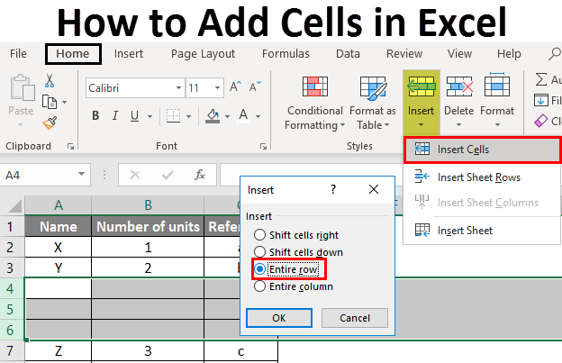
How to Add Cells in Excel (Table of Contents)
- Adding Cells in Excel
- Examples of Add Cells in Excel
Adding Cells in Excel
Adding a cell is nothing but inserting a new cell or group of cells in between the existing cells by using the insert option in excel. We can insert the cells in row-wise or column-wise as per requirement, which allows us to input the additional data or new data in between the existing data.
Explanation: Sometimes, while working with Excel, we may forget to add some portion of date that should be inserted in between the existing data. In that case, we can cut the data and paste it a bit down or right and can input the required data in the gap. However, we can achieve the same without using the cut and paste option but by using the insert option in Excel.
There are four different options available to insert new cells. We will see each option and the respective example.
We can insert new cells in two ways; one way is to select the insert option from the worksheet, and the other is the shortcut key. Click on the “Home” menu at the top left corner in case if you are in a different menu.
After the selection of “Home”, observe the right-hand side we have a section called “cells”. Which covers the options like “Insert”, “Delete”, and “format”, which are highlighted with a red colour box.
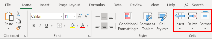
Each option has a drop-down if we observe under each option name. Click on the Insert option drop down then the drop-down menu will appear as below.
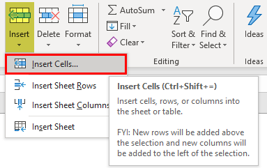
It has four different options: insert cells, insert sheet rows, insert sheet columns, and insert sheet. Click on the option Insert cells; then it will open a pop-up menu with four options as below.
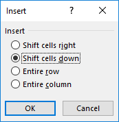
Examples of Add Cells in Excel
Here are some examples of How to Add Cells in Excel, which are given below
You can download this How to Add Cells Excel Template here – How to Add Cells Excel Template
Example #1 – Add a Cell using Shift Cells Right
Consider a table having data of two columns like below.

Now it has three rows of data. But in case if we need to add a cell at the cell B4 by moving the data to the right, we can do that. Follow the steps.
Step 1: Select the cell where you want to add a new cell. Here we have selected B4 as shown below.
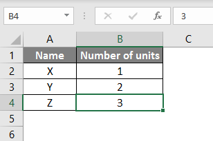
Step 2: Select the Insert menu option for the drop-down as below.
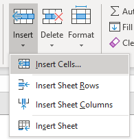
Step 3: Select the Insert Cells option then a pop-up menu will appear as below.
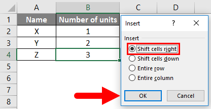
Step 4: Select the “Shift cells right” option, then click on OK. Then the result will appear as below.
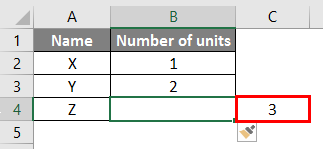
If we observe the above screen, number 3 is shifted to the right and created a new empty cell. This is how “shift cell right” will work. Similarly, we can do the shift cells down also.
Example #2 – Insert a New Column and New Row
To add a new column, follow the below steps. It is as similar to shifting cells.
Step 1: Consider the same table which we took in the above example. Now we need to insert a column in between the two columns.
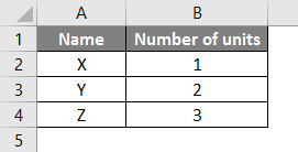
Step 2: A column will always be added on the left-hand side; hence select any one cell in the number of units as below.
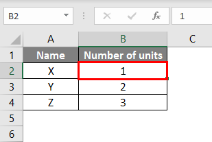
Step 3: Now select the “Entire column” option from the insert option as shown in the below image.
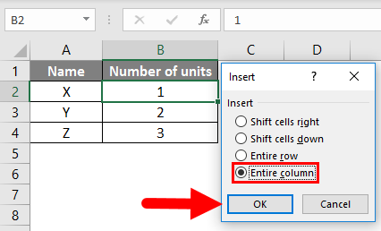
Step 4: Select the OK button. A new column will be added in between the existing two columns as below.
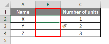
In a similar way, we can add the row by clicking the Entire row option as below.
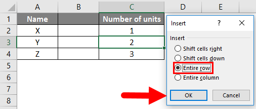
The result will be as below. A new row is added between the data X and Y.
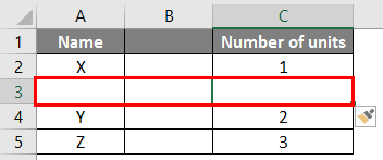
Example #3 – Adding Rows After Each Row using the Sort Option
Up to now, we covered how to add a single cell by shifting cells right and down, adding an entire row an entire column.
But these actions will affect only one row or one column. In case if we want to add an empty row under each existing row, we can perform in another way. Follow the below steps to add an empty row.
Step 1: Take the same table which we used in the previous example.
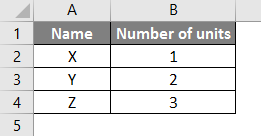
Step 2: Take some reference for the time being column ‘C’ as below.
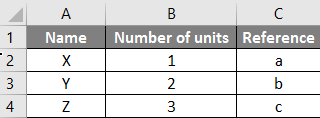
Step 3: Now copy the references and paste them in under the last reference in the table as below.
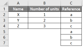
Step 4: To add an empty line under each existing data line, we are using a sorting option. Highlight the entire table and click on the sort option. It is available under “Home”, highlighted in the below picture for reference.
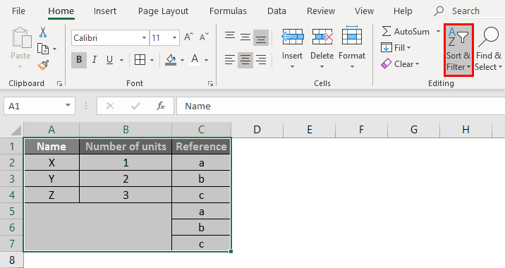
Step 5: From the drop-down of the Sort option, select the custom sort.
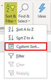
Step 6: A window will open as below.
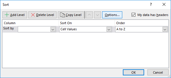
Step 7: From Sort by select the “Reference” option as shown in the below image.
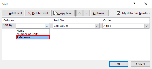
Step 8: Select OK, then see it will sort in such an empty line between each data existing line as below.
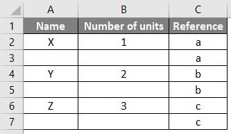
Step 9: Now, we can remove the reference column. I hope you understand why we added the reference column.
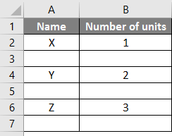
Example #4 – Adding Multiple Rows or Columns or Cells
If we want to add multiple lines or cells at the same time, highlight the number of cells or lines that you required and perform the insert option as per selection. If we select the multiple row lines as below.
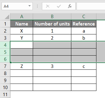
Now use the insert option, which we add for rows.
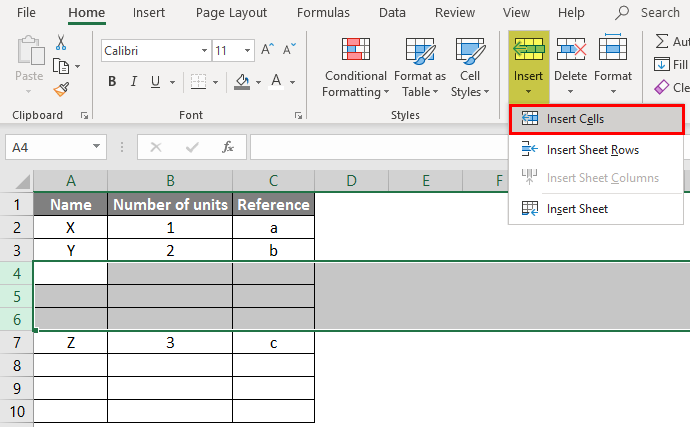
The moment we select “insert cells”, it will directly add the rows without asking for another pop-up as how it asked before. Here we highlighted 3 lines; hence when we click on “Insert Cells”, it will add another 3 empty lines under the selected lines.
Things to Remember
- “Alt + I” is the shortcut key to add a cell or line in the excel spreadsheet.
- A new cell can be added only on the right-hand side and down only. We cannot add the cells to the left and up; hence whenever you want to add the cells to highlight the cell as per this rule.
- A row will always be added at the bottom of the highlighted cell.
- A column will always be added on the left side of the highlighted cell.
- If you want to add multiple cells or rows at a time, highlight multiple cells or rows.
Recommended Articles
This is a guide on How to Add Cells in Excel. Here we discuss How to Add Cells along with examples and downloadable excel template. You may also look at the following articles to learn more –
- How to Sum Multiple Rows in Excel
- SUM Cells in Excel
- Count Cells with Text in Excel
- Excel Shortcut For Merge Cells