
Home / Excel Basics / How to Add Border in Excel
In Excel, a border is like a four-sided line that is added around the cell or range of cells. It is used to highlight a particular area and separate that from the rest of the values on the spreadsheet. Inserting a border draws the focus of the readers to the specific section, which enhances their interest in it.
In this tutorial, we will look at the ways to add borders along with their different types in Excel.
Steps to Apply Borders to a Cell in an Excel
- First, select the cell or group of cells where you want to add a border in your spreadsheet.

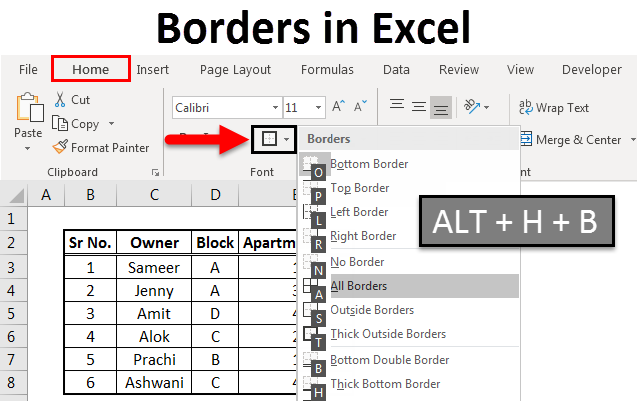
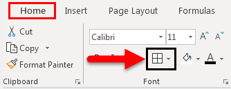
- Then, go to the home tab and in the “Font” group, click on the border button, which is right next to the bold, italic, and underline options.

- Once you click on the drop-down arrow of the border button, it will show you the list of borders.

- Now, select one from the list that you would like to apply around the selected cells.


Types of Borders in Excel
Here, you will learn about the different borders, which are categorized into 4 sections.

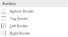
In the first section, there are Bottom, Top, Left, and Right borders. These borders will help you apply only one side border around the single or multiple cells. To apply this to the selected values, just click on any type of border.
In the following example, you can see the bottom border under the scale.

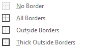
The second section has no border, all borders, outside borders, and thick outside border options. You can easily remove the border from the selected cell by clicking on the no border option.

Next, you have the option to add a border to all four sides of the selected cells. But, with all borders, the border lines separate the cell one by one, as shown in the picture below.

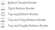
The third section contains many bottom borders. Like, as the bottom double border, thick bottom, top and bottom border, top and thick bottom border, and top and double bottom border.

You can use these options in highlighting or underlining important text or headlines.

Draw the Border
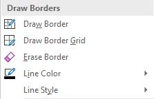
In the last section, you have the option to customize or create the border of your choice by using drawing tools. You can also change the existing border with this.

- Draw Border: Once you click the draw border option, it will convert your cursor into the drawing pencil. Now, click on the cell and drag the left mouse button to insert the border. It applies borders in both directions horizontally and vertically.

- Draw Border Grid: From the name justifies, it is also used to draw a border around the selected cells. But the main difference between the “Draw border” and “Draw border grid” is that the border grid draws the borders in the grid form (On Multiple Cells).

- Erase Border: The eraser helps you to erase the unwanted border line from your cells. To erase the border, you just have to drag the eraser on the line to remove it.

- Line Color: The most amazing thing is you can also change the color of the border to make it more attractive. When you click on the line color, then it will open the pop-up with a variety of colors. Once you pick anyone from this, then use the pencil to draw the colorful border.

- Line Style: To change the style of the borderline, click on the line style and choose one from the following styles.


Advanced Border Options
Choose the advanced borders for your selected cells. Follow the below steps:
- First, go to the “More Borders” option, which is at the bottom of the borders list.
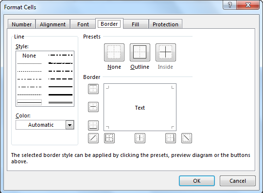
- When you click, it will open a new dialog box called “Format Cells”.

- Here, you have more border options to insert on the sheet.
- And, once you select any given preset, it will also show you how it looks after applying it in the box.

- In the end, click “OK” to apply the selected range of cells.


Remove Borders in Excel
- First, you just need to select the area from which you want to remove the border.
- Then, go to the borders list and select the “No Border” option from there.

- Now, the border lines will disappear around the selected cells.


Shortcut to Add Border
There is another way to add a border by using the shortcut. But before using the shortcut, first, you need to select the range where you want to insert the border.
Then, press ALT ⇢ H ⇢ B simultaneously. Once you do this, you will get the list of borders. Along with this, there are some specific options to set any kind of border on a cell or a range.

You would like to set the Thick Bottom Border and the shortcut key for this is H, as you see in the above screenshot. Then, in this case, press ALT ⇢ H ⇢ B ⇢ H after selecting the data.

Adding cell borders and filling cells with colors and patterns is an easy way to make your data stand out, appear more organized, and make the spreadsheet easier to read.
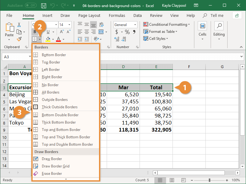
Add a Cell Border
- Select the cell(s) where you want to add the border.
- Click the Border list arrow from the Home tab.
A list of borders you can add to the selected cell(s) appears. Use the examples shown next to each border option to decide which border type will work best for you.
- Select a border type.

To remove a border, click the Border list arrow in the Font group and select No Border.
Advanced Border Options
To have more control over the look and style of the cell borders, use the advanced border options.
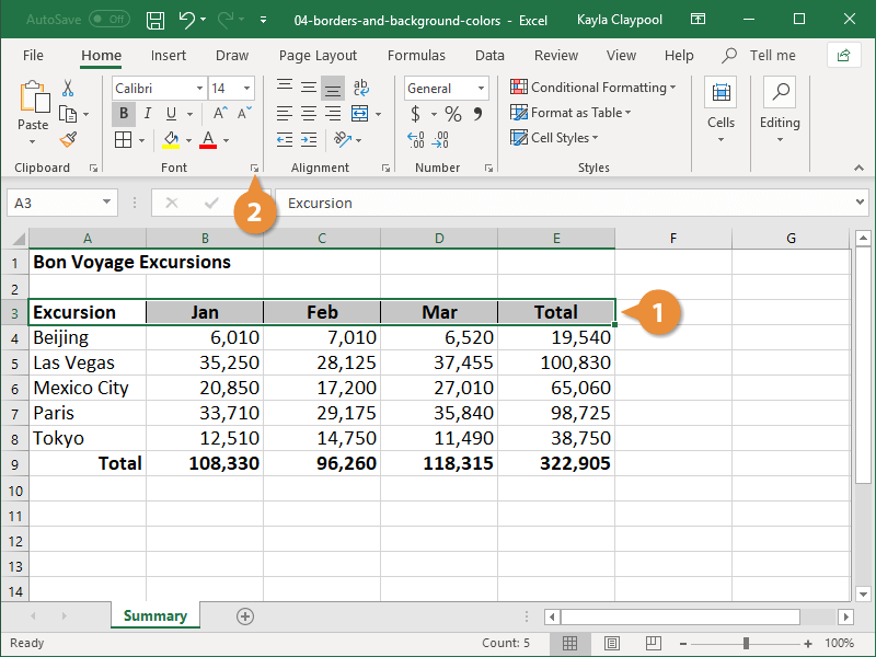
- Select the cell(s) where you want to add the border.
- Click the Font dialog box launcher.
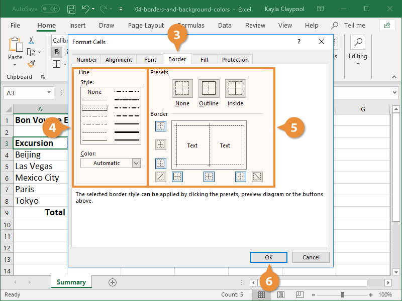
- Click the Border tab.
- Select the line style and color you want.
You now need to specify where you want the new border style to appear.
- Select a preset option or apply borders individually in the Borders section.
- Click OK.
The border is applied to the cell range.
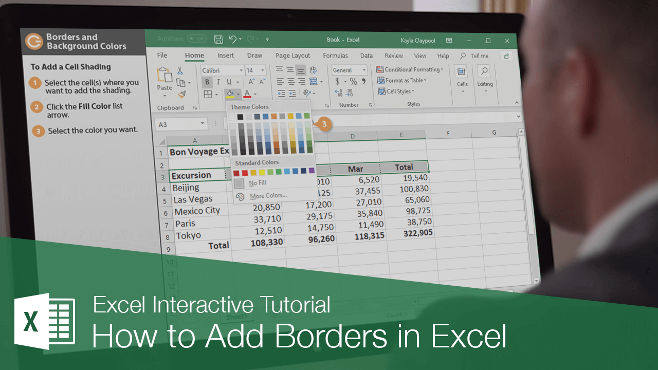
Add Cell Shading
- Select the cell(s) where you want to add the shading.
- Click the Fill Color list arrow.
A palate of theme colors is displayed in the menu. If you want to use a different color, select More Colors.
- Select the color you want to apply.
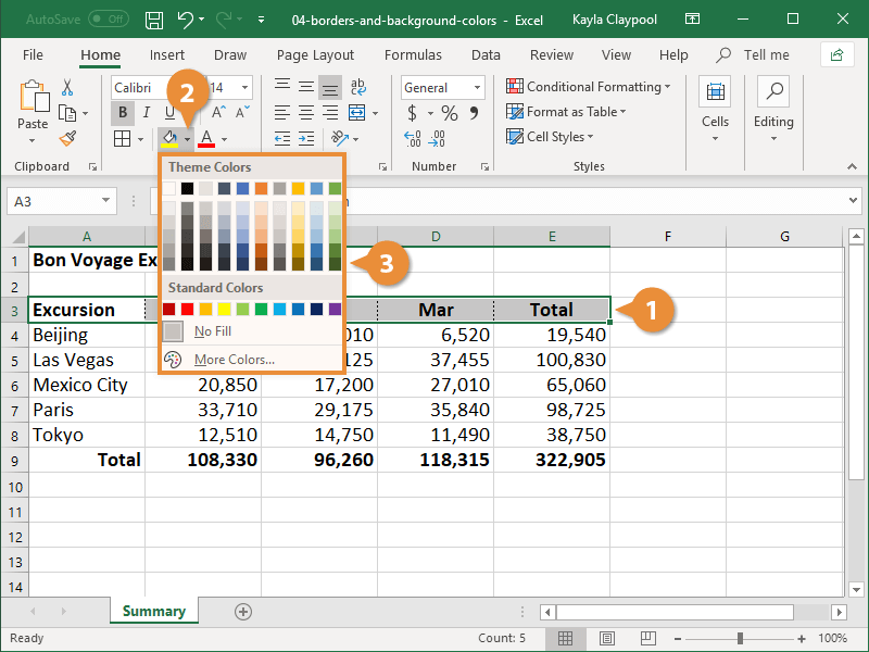
A background color is applied to the cell(s). Make sure the background provides enough contrast with the text to be legible.

FREE Quick Reference
Click to Download
Free to distribute with our compliments; we hope you will consider our paid training.
What are the Borders in Excel?
Borders in Excel are outlined in data tables or a specific range of cells. In Excel, borders are used to separate the data in borders from the rest of the text. It is a good way of representing data. In addition, it helps the user to look for specific data easily. These borders are available in the “Home” tab in the fonts section.
Table of contents
- What are the Borders in Excel?
- Explained
- How to Create and Add Borders in Excel? (with Examples)
- Example #1
- Example #2
- Example #3
- Example #4
- Things to Remember While Creating Borders in Excel
- Recommended Articles
Explained
We can add the border to a single cell or multiple cells. Borders are of different styles and can be used as per the requirement.
Borders help present the data set in a more presentable format in ExcelFormatting is a useful feature in Excel that allows you to change the appearance of the data in a worksheet. Formatting can be done in a variety of ways. For example, we can use the styles and format tab on the home tab to change the font of a cell or a table.read more.
We can use borders for tabular format data or headlines to emphasize a specific set of data or can be used to distinguish different sections.
- We can use it to define or divide the sections of a worksheet.
- We can use it to emphasize specific data.
- We can also make the data more understandable and presentable.
How to Create and Add Borders in Excel? (with Examples)
We can create and add borders to the specific set of data.
Example #1
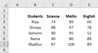
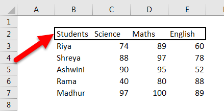
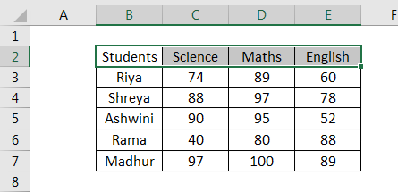
We have data of marks of a student for three subjects of an annual examination. We will have to add the borders in this data to make it more presentable.
- Now, we must select the data we want to add to the borders.

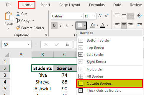
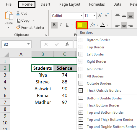
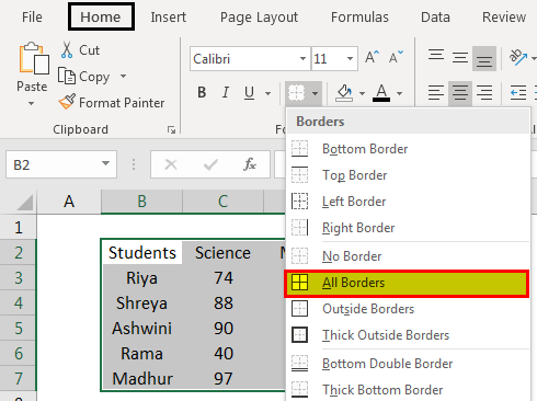
- In the font group on the “Home” tab, click the down arrow next to the “Borders” button. You may see the drop-down list of borders, as shown in the figure below.

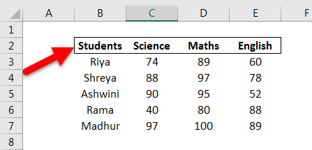
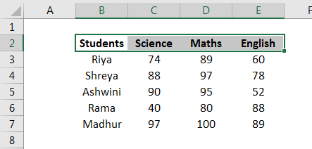
- We have different borders styles. Therefore, we may select the “OUTSIDE BORDERS” option for our data.

- We may find the result by using “OUTSIDE BORDERS” in the data.

Now, let us learn with some more examples.
Example #2
We have data of marks of a student for three subjects of an annual examination. We will have to add the borders in this data to make it more presentable.
- Data of marks of 5 students for three subjects in an annual examination is shown below.
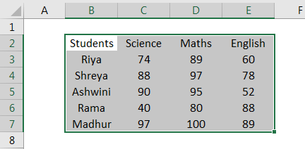
- Now, we must select the data we want to add to the borders.
- Now, in the “Font” group on the “Home” tab, we need to click the down arrow next to the “Borders” button. As shown in the figure below, we may see the drop-down list of borders.
- Now that we have different border styles, we must select the “THICK OUTSIDE BORDERS” option for data.
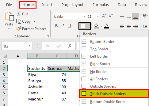
- As a result, we may find the result by using “THICK OUTSIDE BORDERS” to the data shown below.
Example #3
We have data on the marks of a student for three subjects of an annual examination. We will have to add the borders in this data to make it more presentable.
- Data of marks of 5 students for three subjects in an annual examination is shown below.
- Now, select the data to which you want to add borders.
- Now, in the “Font” group on the “Home” tab, we may need to click the down arrow next to the “Borders” button. And we may see the drop-down list of borders as shown in the figure below. Then, select the “ALL BORDERS” options for the data.
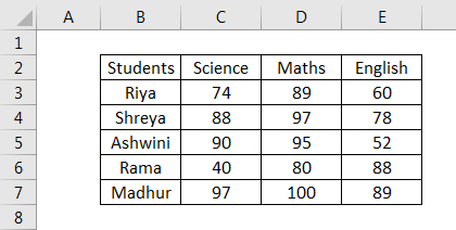
- As a result, we may find the result by using “ALL BORDERS” to the data.
Example #4
We have data on the marks of a student for three subjects of an annual examination. We need to add the borders in this data to make it more presentable.
- Data of marks of 5 students for three subjects in an annual examination is shown below.
- Now, we must select the data we want to add borders.
- Now, in the “Font” group on the “Home” tab. Then, we need to click the down arrow next to the “Borders” button. As shown in the figure below, we may see the drop-down list of borders. Now, select the “ALL BORDERS” options for our data.
- We may now find the result using “ALL BORDERS” in the data.
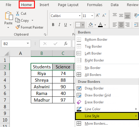
- As shown in the figure below, we can change the border’s thickness per the requirement. Select the data you want to change the border’s thickness for this.
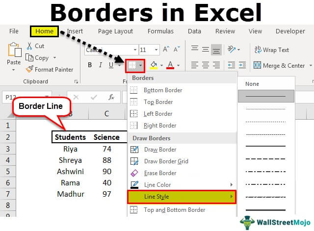
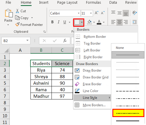
- We need to go to the border drop-down list and click “LINE STYLE.”
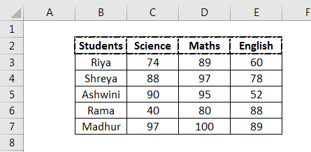
- Now, we get a list of line styles and use the style as per the requirements. We will use the second last line style for our data.
- We may get the result as shown below.
Things to Remember While Creating Borders in Excel
- We select cells where the border needs to be added.
- The borders differentiate the data separately.
- We can change border styles by the “Borders” icon in the “Font” tab.
Recommended Articles
This article has been a guide to Borders in Excel. Here, we discuss how to create/add cell borders in Excel using different options and examples. You may also look at these useful functions in Excel: –
- Borders in VBA Excel
- VBA Select Cell
- Shortcut for Excel Format Painter
- Format Number in VBA
- Marksheet in Excel
Reader Interactions
Excel Borders (Table of Contents)
- Borders in Excel
- How to add Borders in Excel?
Borders in Excel
Borders are the boxes formed by lines in the cell in Excel. By keeping borders, we can frame any data and provide them with a proper define limit. To distinguish specific values, outline summarized values or separate data in ranges of cells; you can add a border around cells.
How to add Borders in Excel?
Adding borders in Excel is very easy and useful to outline or separate specific data or highlight some values in a worksheet. Normally, we can easily add all top, bottom, left, or right borders for selected cells in Excel. Option for Borders is available in the Home menu, under the font section with the icon of Borders. We can also use shortcuts to apply borders in Excel.
You can download this Borders Excel Template here – Borders Excel Template
Let’s understand how to add Borders in Excel.
Example #1
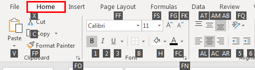
For accessing Borders, go to Home and select the option as shown in the below screenshot under the Font section.
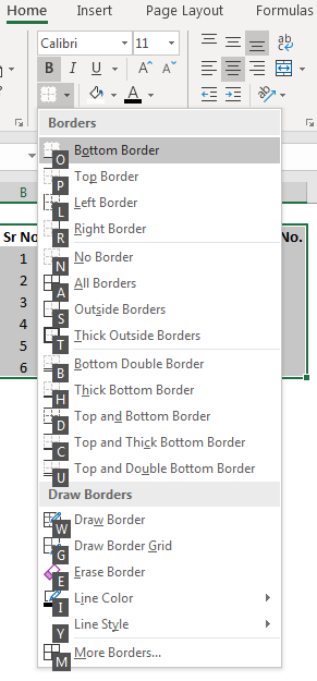
Once we click on the option of Borders shown above, we will have a list of all kind of borders provided by Microsoft in its drop-down option, as shown below.
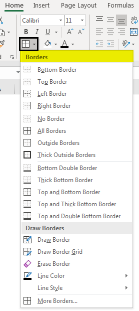
Here we have categorized Borders into 4 sections. This would be easy to understand because all sections are different from each other.
The first section is a basic section with only Bottom, Top, Left, and Right Borders. By this, we can only create one side border only for one cell or multiple cells.
The second section is the full border section, which has No Border, All Borders, Outside Borders, and Thick Box Borders. By this, we can create a full border that can cover a cell and a table as well. We can also remove the border as well from the selected cell or table by clicking on No Border.
The third section is a combination of the bottom borders, Bottom Double Border, Thick Bottom Border, Top and Bottom Border, Top and Thick Bottom Border, and Top Double Bottom Border.
These types of double borders are majorly used in underlining the headlines or important texts.
The Fourth section has a customized border section, where we can draw or create a border as per our need or make changes in the existing border type. We can change the color, thickness of the border as well in this section of Borders.
Once we click on the More Borders Option at the bottom, we will see a new dialog box named Format Cells, which is a more advanced option for creating Borders. It is shown below.
Example #2
We have seen the basic function and use for all kinds of borders and how to create those in the previous example. Now we will see an example where we will choose and implement different Borders and see how those Borders in any table or data can be framed.
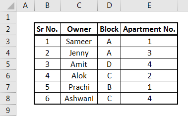
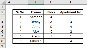
We have a data table, which has details of Owner, Block, and Apartment No. Now we will frame the Borders and see how the data would look like.
As row 2 is the headline, we will prefer a double bottom line selected from the third section.
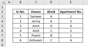
And all cell will be covered with a box of All Borders which can be selected from the second section.
And if we select Thick Border from the second section, then the whole table will be bound to a perfect box, and selected data will automatically get highlighted. Once we are done with all the mentioned border type, our table would like this, as shown below.
As we can see, the complete data table is getting highlighted and ready to be presented in any form.
Example #3
There is another way to frame borders in excel. This is one of the shortcuts of accessing the functions available in excel. For accessing borders, the shortcut way first selects the data we want to frame with borders and then press ALT + H + B simultaneously to enable the border menu in Excel.

ALT + H will enable the Home menu, B will enable the borders.

Once we do that, we will get a list of all kinds of borders available in excel. And this list itself will have the specific keys mentioned to set for any border as shown and circled in the below screenshot.
We can navigate to our required Border type by pressing the Key highlighted in the above screenshot, or else we can use direction keys to scroll up and down to get the desired border frame. Let’s use All Borders for this case by pressing ALT+H+B+A simultaneously after selecting the data table. Once we do that, we will see the selected data is now framed with all borders. And each cell will be now having its own border in black lines, as shown.
Let’s frame one more border of another type with the same process. Select the data first and then press ALT+H+B+T Keys simultaneously. We will see that data is framed with Thick Borders, as shown in the below screenshot.
Pros of Print Borders in Excel
- Creating the border around the desired data table makes data presentable to anyone.
- Border frame in any data set is quite useful when printing the data or pasting the data in any other file. By this, we make the data look perfectly covered.
Things to Remember
- Borders can be used with the shortcut key Alt + H + B, which will directly take us to the Border option.
- Giving a border in any data table is very important. We must provide the border after every work so that the data set can be bound.
- Always make proper alignment so that once we frame the data with a border and use it in different sources, the column width will be automatically set.
Recommended Articles
This has been a guide to Borders in Excel. Here we discussed how to add Borders in Excel and use shortcuts for borders in Excel along with practical examples and a downloadable excel template. You can also go through our other suggested articles –
- LEFT Formula in Excel
- VBA Borders
- Format Cells in Excel
- Print Gridlines in Excel
(Note: This guide on how to add borders in Excel is suitable for all Excel versions including Office 365)
Excel is one of the most popular data-handling applications. When working with large amounts of different data types, you might need to differentiate the data. To differentiate the data, Excel offers a variety of formatting options. One of the useful formatting options to differentiate, highlight, and showcase data is by using borders
In this article, I will tell you how to add borders in Excel in 3 easy ways. You’ll also learn how to remove the applied borders.
You’ll Learn:
- What Are Borders in Excel?
- How to Add Borders in Excel?
- Apply Built-In Borders
- Create and Apply a Custom Cell Border
- Draw a Cell Border
- Remove the Cell Border

Related Reads:
HOW TO CHANGE THE MARGINS IN EXCEL? 2 USEFUL WAYS
HOW TO USE CELL STYLES IN EXCEL: A STEP-BY-STEP GUIDE
HOW TO INDENT IN EXCEL? 3 EASY METHODS
What Are Borders in Excel?
Before we learn how to add borders in Excel, let us see what borders are in Excel.
Borders are a line around a cell or a group of cells in Excel. They are mainly used to highlight particular data among a group of data. By default, Excel does not have any borders and the cell circumference is the only differentiating factor. However, you can apply a variety of borders to your spreadsheet to differentiate the data in the cells.
Borders can also be used to create tables, and group similar data or sections in a worksheet together.
By default, Excel prints any borders applied to the worksheets. In case you don’t want the printed sheets to appear with the borders, you can choose to remove them.
How to Add Borders in Excel?
In Excel, you can add cell borders of different types and sizes depending on your preferences. You can either choose to add the built-in borders or choose the custom borders based on your choice.
Let us now see how to add borders in Excel worksheets in detail with an example. Consider an Excel worksheet that has the data of students in a particular class and the marks they scored in 5 subjects. Along with the marks, the table also houses the total and average marks scored by each student.

At first glance, the data looks all the same without any differentiation in the important data. To ascertain the data easily, let us add borders to the given data.
Apply Built-In Borders
You can easily select and add built-in borders in Excel with just a few clicks.
- First, open the Excel worksheet and select a cell or a group of cells for which you want to apply the borders.
- Navigate to Home. Under the Font section, you can find the Borders option which appears between the underline and highlight buttons.

- You will find that the border button highlights the most recent border option you have used. When you want to use that particular border, you can just click on the border button.
- If you want to explore and use a different border, click on the dropdown next to the borders button.

- From the dropdown, you can find multiple options to apply borders and additional options to draw and customize them.
Note: When you apply cell borders to the cells, you will notice that the border is also applied to the adjacent cells. In case you have applied two different borders to the adjacent cells, the cell border of the recent selection is applied.
Suggested Reads:
HOW TO INSERT IMAGE IN EXCEL? 3 EASY WAYS
HOW TO REMOVE DOTTED LINES IN EXCEL? 3 DIFFERENT CASES
HOW TO SPLIT CELLS DIAGONALLY IN EXCEL? 2 EASY WAYS
Create and Apply a Custom Cell Border
Excel offers options to choose and apply any built-in cell borders. However, in some cases, you might want a different cell border of your choice. In those cases, you can customize a cell border and use it whenever needed.
- To create a custom cell border, select the cells you want to apply the border.
- Navigate to the Home main menu ribbon. Under the Styles section, click on the dropdown from Cell Styles and click on New Cell Style.

- This opens the Styles dialog box. In the dialog box, name your style and select the areas where you want to apply the border. Then, click on the Format button.

- Click on the Border tab. Choose the border line styles, presets, and colors.
- Finally, click OK.

- Again, click OK.
- You can find the new cell border from the Home main menu, under the Cell Styles option. From the dropdown, click on the cell style you created under the Custom section.

Draw a Cell Border
There is another way to apply borders to cells in Excel. In this method, you can easily draw the borders over the cells.
- To draw borders, first, choose the Line Style and the Line Color from the Borders dropdown in the Home main menu ribbon.
- Then, click on the Draw Border or Draw Border Grid to enable the pencil icon. The Draw Border option draws the outline borders, whereas, the Draw Border Grid is used to draw the outer, as well as, inner borders.

- Click and drag the mouse pointer over the cells to apply the borders.

- Once the borders are drawn, click on Home and again click on the border button to disable the border pen.
Remove the Cell Border
Cell borders are a great addition to your presentation to highlight and showcase the data. However, some cases might not need a cell border. There are two ways to remove a cell border.
One way to remove a cell border is by clicking on the No Border option.
- To remove the borders, first, select the cells with the borders.
- Click on the Home main menu ribbon. Under the Borders dropdown, click on No Border.

- This instantly removes the border from the selected cells.
Another way to remove the borders is by erasing them manually.
- To erase the applied borders, click on the Home main menu. Under the Borders dropdown, click on the Erase Border option.
- Once the eraser icon is enabled, you can click and drag on the cells to clear the borders.

Also Read:
HOW TO COPY ONLY VISIBLE CELLS IN EXCEL? 3 EASY WAYS
HOW TO PRINT GRIDLINES IN EXCEL?
HOW TO MAKE A SANKEY DIAGRAM EXCEL DASHBOARD? A STEP-BY-STEP GUIDE
Frequently Asked Questions
How to add borders in Excel easily?
First, select the cells. Then, click on the Borders button or dropdown from the Home main menu ribbon to add borders to the selected cells.
How to remove borders in Excel?
To remove the added borders in Excel, first, select the cells with borders. Then navigate to Home main menu, click on the dropdown from Borders, and click on No Borders.
How do I customize the borders in Excel?
To add custom borders, first, select the cells. Then, click on the dropdown from Borders and select More Borders or right-click on the cells and select Format Cells. From the dialog box, click on the Border tab and customize them. You can also click on Home and create a custom cell style selecting the border of your preference.
Closing Thoughts
By adding borders to cells in Excel, you can highlight the particular information that can easily be ascertained by the reader without much effort. It can also be used to highlight any important data which signifies the consolidated result.
In this article, we saw how to add borders in Excel in 3 easy ways. We also saw how to customize the borders and remove them when not necessary.
Want more high-quality guides for Excel? Check out our free Excel resources centre.
Click here to access in-depth Excel training courses and master in-demand advanced Excel skills.
Simon Sez IT has been teaching critical IT software for over ten years. For a low, monthly fee you can get access to 150+ IT training courses by seasoned professionals.

Simon Calder

Chris “Simon” Calder was working as a Project Manager in IT for one of Los Angeles’ most prestigious cultural institutions, LACMA.He taught himself to use Microsoft Project from a giant textbook and hated every moment of it. Online learning was in its infancy then, but he spotted an opportunity and made an online MS Project course — the rest, as they say, is history!
When working with large amounts of data, it can sometimes be hard to read the data, if not formatted properly.
Moreover, there are usually parts of the dataset that are more important than others, so you would want these cells to stand out from the rest. This can get the reader to concentrate more on the important areas of the dataset.
There are a number of ways to improve the readability of your data. A very effective way is to add borders around the cells.
Borders can also be customized to highlight important cells. For example, you can use a thicker border to make the Grand total or some important data value stand out.
Excel provides several options for cell borders. In this tutorial, I will show you three different ways to apply borders to cells in Excel.
The options you choose and how you apply them to your spreadsheets will be up to your creativity. But I can guarantee you this, you’ll be spoilt for choice.
Say we have a dataset as the one given below.

We notice two things here:
- The cells do have gridlines, but they could be more readable if there were borders around every cell containing data.
- The most important cell in this dataset is the Grand Total. So, it would help if we could make this particular cell more pronounced by adding a thicker border around it.
There are three ways to add and customize cell borders in Excel:
- By accessing the Border button from the Home tab
- By accessing the Format Cell dialog box’s Border tab.
- By manually drawing the borders.
We are going to take a look at each of the above ways one by one.
How to Add Borders from the Home Tab
- Select the cells around which you want to add borders. To select individual cells, press down the control key, and select each cell. To select a group of cells, drag your mouse over the group of cells you want to select.
- Click the arrow next to the Borders button. You will find it in the Home tab, under the ‘Font’ group.

- A dropdown menu should now appear. This will contain quick border options that you can apply to your selected cells. In our dataset, we applied simple grid-like single borders around each cell. We also added a thick border around the grand total to make it stand out.
Here’s how the dataset looks after applying borders:

The borders provided an instant ‘lift’ to the entire dataset.
The Borders button dropdown provides a selection of common border options that you can quickly apply to your selection. You can choose to have individual borders on the top, bottom, left, or right. You can also combine 2 to 3 borders or have all 4 borders for each selection.
Additionally included in this menu are options for various border styles, like thick border, double border, and other common border combinations.

If you want more options, though, you can navigate to the Format Cells dialog box.
How to Add Borders from the Format Cells Dialog Box
Another way to add borders to cells or ranges is to use the Format Cells dialog box. While it has many of the same options to apply borders, you get access to many more additional options as well.
For example, here’s just a glance at the dialog box’s Border tab:

- On the left of the dialog box, there’s a ‘Style’ section, where you can select the type of border you want, like dashed, dotted, thick, double, and more.
- The ‘Color’ section is also present on the left side. As the name suggests, this lets you select the color you want for the borders.
- The right side top portion has some ‘Presets’ that you can select to quickly add borders either in between cells or around cells.
- The lower portion of the right side is the main ‘Border’ section. This lets you select which parts of your selection you want your borders on.
- This section also provides a small preview of how your selections are going to look when you apply your choice of borders on them.
There are a number of ways to open the Format Cells Dialog box:
Here are the steps to follow when you want to add borders using the Format Cells dialog box:
- Use any of the above methods to open the ‘Format Cells’ Dialog box.
- Select the Border tab.
- Here you will see a whole assortment of border options that you can play around with. For our example, we made the following selections:
- An orange accent line color
- A dashed line style
- The Outline preset
- The Inside preset

- When you’re done putting all your border settings, click OK to close the dialog box. Your borders will now get applied to your selections.


How to Add Borders by Manually Drawing Them
Finally, if you want more control over individual borders, you can use the ‘Draw Borders’ feature of Excel.
Draw Borders gives you the flexibility to draw even irregular shaped border, something that can be quite tough to do using the Format Cells dialog box.
Here’s a quick look at the different options you get under the Draw Borders feature:

- Draw Border: This lets you draw a border along any gridline. When you select a block of cells in this mode, it creates a rectangular border around the outside of the selected block of cells.
- Draw Border Grid: This also lets you draw a border along any gridline, but when you select a block of cells in this mode, it creates borders both inside and outside the block of cells (to form a grid).
- Erase Border: This lets you erase any previously created borders individually or collectively.
- Line Color: This lets you select the color of the individual borders.
- Line Style: This lets you select the type of individual borders, like dashed, dotted, thick, double, etc.
Here’s how to use the Draw Borders feature:
- Since you are going to manually draw individual borders one by one, you don’t need to have any cells selected.
- Click the arrow next to the Borders button. You will find it in the Home tab, under the ‘Font’ group.
- From the dropdown menu that appears, navigate down to the ‘Draw Borders’ section.

- First, select the line color

- And then select the border style

- Notice that as soon as you select an option from the Draw Borders section, your mouse pointer turns into a pencil, to tell you that you are now in ‘Draw Border’ mode.

- Go ahead and draw your borders along any gridline you like. You can even create a rectangular border by clicking and dragging around any block of cells. We have chosen to just draw two thick borders above and below the grand total.
- Once you’re done drawing all your required borders, you can come out of the border drawing mode by clicking on the Border button (under the Home tab) again.


Here is what our dataset looks like after drawing borders above and below the grand total:

The Difference between Borders and Gridlines
Before you start applying borders to your cells, it is important to understand the basic difference between borders and gridlines.
Gridlines are the light-colored boxes around every cell in your sheet. They are there to help define individual cell borders. In Excel, there are options to show or hide the gridlines when you take a print of your worksheet.
Borders, on the other hand, help to accent a cell or set of cells. So even if you choose not to display gridlines in your printout, your borders will remain visible and get printed, unless you remove them.
Additionally, when you hide gridlines in the Excel window, they get hidden for the entire worksheet. But with borders, you can choose to have them displayed on specific cells or ranges, even when gridlines are hidden.
Also read: How to Remove Borders in Excel? 6 Easy Ways!
So, in this Excel tutorial, I showed you three ways in which you can add borders to your cells, both individually and in bulk.
I would encourage you to experiment with the different border settings to see which style suits you and your data.
You can also use these border settings to create your own signature style for highlighting important cells in spreadsheets.
I hope you found this tutorial useful!
Other Excel tutorials you may find useful:
- How to AutoFormat Formulas in Excel (3 Easy Ways)
- How to Highlight Every Other Row in Excel
- How to Set the Default Font in Excel (Windows and Mac)
- How to Remove Dotted Lines in Excel
- How to Flash an Excel Cell
- How to Remove Panes in Excel Worksheet (Shortcut)
- How to Add a Total Row in Excel Table
- How to Add Bullet Points in Excel
- How to Change Theme Colors in Excel?
- How to Add Border to a Chart in Excel
Want to add borders in Excel to clearly display specific data tables? Borders play an important role in tabular data representation. It helps classify headings and contents of a table for better interpretation of information.
Adding or removing borders in Excel is simple and easy. This article is a complete guide to adding borders to any kind of tabular data available to you.
Recommended read: Steps to clear formatting in Excel
Let’s get started with learning to add or remove borders in Excel through this tutorial, step by step.
1. Create a database
First, we take a small database to begin adding borders to the tabular data. Here is an example of a tabular database-
 3")
2. Add borders to Excel database
This database can look more systematic and neat with borders around it. Here’s how to add borders-
- Select the complete database.
 4")
- Select the type of bordering you like for your table. We have selected All Borders.
 5")
- You can add a different kind of border for headings. We have selected Thick Outside Borders.
 6")
- Select No Border, if you want to remove applied borders on selected cells.
 7")
3. Drawing a border in Excel
You can have more border options like Top, Bottom, Left or Right border styles in excel for your tabular data.
Well, that’s not all, you can even draw your own borders the way you want them, under the Draw Borders section of border options in excel.
- Select Draw Border to draw border lines for one or more sides of a cell (left, right, top or bottom).
 8")
- Select Draw Border Grid to add borders to all sides of a cell at once.
 9")
- If you want to remove drawn borders from cells, you can either select the Erase Border option or No Border option after selecting those cells.
 10")
- To draw borders in custom colors, select Line Color.
 11")
4. More Border Options in Excel
The More Border Options can be found in the bottom of border options in excel which allows you to fully customize your borders the way you like.
 12")
You can even customize the setup to selecting a custom color and style for each side of your borders and grids manually.
 13")
- You can see how fully custom colored and styled is each side of the border in this image.
- To apply a color or style to a side select the color or style you like and click on the side of your border in the preview.
- To remove applied borders, select cells with borders and apply the No Border option.
Conclusion
This was all about adding or removing borders in Microsoft Excel to any kind of tabular data in hand. Use borders to beautify your tables and make them look presentable. Follow these steps to create a professional-looking database. Drop a comment if you got any questions regarding borders in Excel!
Select the cells you want to format. Click the down arrow beside the Borders button in the Font group on the Home tab. A drop-down menu appears, with all the border options you can apply to the cell selection. Use the Borders button on the Home tab to choose borders for the selected cells.
Contents
- 1 What is the shortcut for all borders in Excel?
- 2 How do I automatically add gridlines in Excel?
- 3 Where do you find all borders in Excel?
- 4 What is Ctrl D in Excel?
- 5 How do you repeat borders in Excel?
- 6 How do you add a dynamic border in Excel?
- 7 How do I automatically outline a column in Excel?
- 8 How do you outline cells in Excel 2020?
- 9 What is Accent 6 Excel?
- 10 What is Ctrl M in Excel?
- 11 What is the fastest way to add a border in Excel?
- 12 What is Ctrl J in Excel?
- 13 Why is Excel adding borders automatically?
- 14 How do I underline every row in Excel?
- 15 How do you add borders in Excel 2016?
- 16 How do I create multiple groups in Excel?
- 17 Why can’t I create an auto outline in Excel?
- 18 How do you apply all borders?
- 19 Why can’t I put borders around cells in Excel?
- 20 How can you add a border around a set of cells covering several rows and columns?
What is the shortcut for all borders in Excel?
Alt + H + B + A: All borders.
How do I automatically add gridlines in Excel?
How to add borders automatically to cells in Excel?
- Add borders automatically to cells with Conditional Formatting.
- Select the range of cells that you want the gridlines to appear on rows when you enter values.
- From the Home tab, click Conditional Formatting > New Rule, see screenshot:
Where do you find all borders in Excel?
- Click the arrow on the button that looks like a little window, this is call the ‘Borders’ button, this will open up a drop down list.
- Click on the ‘All Borders’ choice.
What is Ctrl D in Excel?
Ctrl+D in Excel and Google Sheets
In Microsoft Excel and Google Sheets, pressing Ctrl + D fills and overwrites a cell(s) with the contents of the cell above it in a column. To fill the entire column with the contents of the upper cell, press Ctrl + Shift + Down to select all cells below, and then press Ctrl + D .
How do you repeat borders in Excel?
Copy and paste these styles with Excel’s Format Painter tool.
- Click the upper-left cell in the range with the border you want to copy.
- Drag your cursor to the range’s lower-right cell, selecting the entire range.
- Click “Home” on Excel’s menu bar.
- Click the “Format Painter” icon from the ribbon’s Clipboard tab.
How do you add a dynamic border in Excel?
How to create dynamic border
- Select the top cells of your list.
- Go to “Home” tab in excel 2007.
- Press with left mouse button on the small triangle on the border button in the font window. See picture below.
- Press with left mouse button on “Top border”
How do I automatically outline a column in Excel?
Select a cell in the range of cells you want to outline. On the Data tab, in the Outline group, click the arrow under Group, and then click Auto Outline.
How do you outline cells in Excel 2020?
To outline Excel data by applying an outline to a selected range of cells, select the cell range to outline. Then click the “Data” tab in the Ribbon. Then click the “Group” button in the “Outline” button group to launch the “Group” dialog box.
What is Accent 6 Excel?
Orange color (accent 6, darker 50%)
– Select your particular cells assume that, A1:H16. – Select background color as Red with black border and Click ok. – Select background color as Orange and Click ok.
What is Ctrl M in Excel?
In Microsoft Word and other word processor programs, pressing Ctrl + M indents the paragraph. If you press this keyboard shortcut more than once, it continues to indent further. For example, you could hold down the Ctrl and press M three times to indent the paragraph by three units.
What is the fastest way to add a border in Excel?
Here’s how:
- Select a cell or a range of cells to which you want to add borders.
- On the Home tab, in the Font group, click the down arrow next to the Borders button, and you will see a list of the most popular border types.
- Click the border you want to apply, and it will be immediately added to the selected cells.
What is Ctrl J in Excel?
Using Find & Replace to insert line breaks (CTRL+J) erases cell contents.
Why is Excel adding borders automatically?
That is because cell A1 is not blank, so the formatting is applied. As I enter data, the borders automatically appear. As I keep entering data, borders keep appearing. If I take out what is in column A, the entire row loses its borders due to the way the formula was set up.
How do I underline every row in Excel?
Underline all or selected cell contents
- Do one of the following: To underline all text or numbers in a cell or range of cells, select that cell or range of cells.
- On the Home tab, in the Font group, do one of the following: To apply a single underline, click Underline .
How do you add borders in Excel 2016?
MS Excel 2016: Draw a border around a cell
- Right-click and then select “Format Cells” from the popup menu.
- When the Format Cells window appears, select the Border tab. Next select your line style and the borders that you wish to draw.
- Now when you return to your spreadsheet, you should see the border, as follows:
- NEXT.
How do I create multiple groups in Excel?
To group rows or columns:
- Select the rows or columns you want to group. In this example, we’ll select columns A, B, and C.
- Select the Data tab on the Ribbon, then click the Group command. Clicking the Group command.
- The selected rows or columns will be grouped. In our example, columns A, B, and C are grouped together.
Why can’t I create an auto outline in Excel?
If you receive a pop-up box that says “Cannot create an outline”, your data doesn’t have an outline-compatible formula in it. You’ll need to manually outline the data.
How do you apply all borders?
Click the down arrow beside the Borders button in the Font group on the Home tab. A drop-down menu appears, with all the border options you can apply to the cell selection. Use the Borders button on the Home tab to choose borders for the selected cells. Click the type of line you want to apply to the selected cells.
Why can’t I put borders around cells in Excel?
If you apply the borders to cells that will be hidden, then the borders will NOT be visible when the rows or columns are hidden. Even if the adjacent rows or columns are visible, the border will be hidden because it was applied to the cells that are hidden.
How can you add a border around a set of cells covering several rows and columns?
How can you quickly add a border around a set of cells covering 3 rows and 12 columns? Use Draw Border under Border on the ribbon under Home.