
Use a screen reader to add, remove, or arrange fields in a PivotTable in Excel
Excel for Microsoft 365 Excel for the web Excel 2021 Excel 2019 Excel 2016 Excel Web App More…Less
This article is for people with visual or cognitive impairments who use a screen reader program such as Microsoft’s Narrator, JAWS, or NVDA with Microsoft 365 products. This article is part of the Microsoft 365 screen reader support content set where you can find more accessibility information on our apps. For general help, visit Microsoft Support home.
Use Excel with your keyboard and a screen reader to add or remove fields in a PivotTable using the PivotTable Fields pane. We have tested it with Narrator, NVDA, and JAWS, but it might work with other screen readers as long as they follow common accessibility standards and techniques. You’ll also learn how to rearrange the fields to change the design of a PivotTable.
Notes:
-
New Microsoft 365 features are released gradually to Microsoft 365 subscribers, so your app might not have these features yet. To learn how you can get new features faster, join the Office Insider program.
-
To learn more about screen readers, go to How screen readers work with Microsoft 365.
In this topic
-
Open the PivotTable Fields pane manually
-
Add fields to a PivotTable
-
Remove fields from a PivotTable
-
Arrange fields in a PivotTable
Open the PivotTable Fields pane manually
The PivotTable Fields pane should automatically appear when you place the cursor anywhere in the PivotTable. To move the focus to the pane, press F6 repeatedly until you hear: «PivotTable fields, Type field name to search for.» If you do not hear that and the focus cycles back to the selected cell instead, you need to manually open the pane.
-
Place the cursor in any cell in your PivotTable.
-
Press Alt+J, T, then L. The PivotTable Fields pane opens.
Add fields to a PivotTable
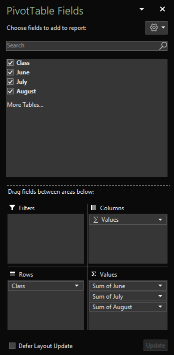
In the PivotTable Fields pane, you can pick the fields you want to show in your PivotTable.
-
On the worksheet with the PivotTable, place the cursor in any cell in your PivotTable, and press F6 until you hear: «PivotTable fields, Type field name to search for.»
-
To browse the list of available fields, use the Down or Up arrow key. You hear the name of the field and if it’s unselected or selected. Unselected fields are announced as «Checkbox unchecked.»
-
When you land on an unselected field you want to add to your PivotTable, press Spacebar. The field and its data are added to the PivotTable on the worksheet grid. Repeat this step to all fields you want to add to the PivotTable.
The fields you select are added to their default areas: non-numeric fields are added to Rows, date and time hierarchies are added to Columns, and numeric fields are added to Values.

Remove fields from a PivotTable
In the PivotTable Fields pane, you can unselect the fields you don’t want to show in your PivotTable. Removing a field from a PivotTable doesn’t remove the field from the PivotTable Fields pane or delete the source data.
-
On the worksheet with the PivotTable, place the cursor in any cell in your PivotTable, and press F6 until you hear: «PivotTable fields, Type field name to search for.»
-
To browse the list of available fields, use the Down or Up arrow key. You hear the name of the field and if it’s unselected or selected. Selected fields are announced as «Checkbox checked.»
-
When you land on a selected field you want to remove from your PivotTable, press Spacebar. The field and its data are removed from the PivotTable. Repeat this step to all fields you want to remove from the PivotTable.
Arrange fields in a PivotTable
To rearrange the fields to match how you want them displayed in the PivotTable, you can move a field from one area to another. You can also move a field up or down within an area.
-
In the PivotTable Fields pane, press the Tab key until you hear the name of the field you want to move, followed by «Button.»
-
Press Spacebar to open the context menu.
-
Press the Up or Down arrow key until you hear the option you want, for example, «Move to column labels» or «Move up,» and press Enter. The PivotTable on the grid is updated accordingly.
The fields in the different areas in the PivotTable Fields pane are shown in the PivotTable as follows:
-
The fields in the Filters area are shown as top-level report filters above the PivotTable.
-
The fields in the Columns area are shown as Column Labels at the top of the PivotTable. Depending on the hierarchy of the fields, columns might be nested inside other columns that are higher in the hierarchy.
-
The fields in the Rows area are shown as Row Labels on the left side of the PivotTable. Depending on the hierarchy of the fields, rows might be nested inside other rows that are higher in the hierarchy.
-
The fields in the Values area are shown as summarized numeric values in the PivotTable.
See also
Use a screen reader to filter data in a PivotTable in Excel
Use a screen reader to group or ungroup data in a PivotTable in Excel
Keyboard shortcuts in Excel
Basic tasks using a screen reader with Excel
Set up your device to work with accessibility in Microsoft 365
Use a screen reader to explore and navigate Excel
What’s new in Microsoft 365
Use Excel for the web with your keyboard and a screen reader to add or remove fields in a PivotTable using the PivotTable Fields pane. We have tested it with Narrator in Microsoft Edge and JAWS and NVDA in Chrome, but it might work with other screen readers and web browsers as long as they follow common accessibility standards and techniques. You’ll also learn how to rearrange the fields to change the design of a PivotTable.
Notes:
-
If you use Narrator with the Windows 10 Fall Creators Update, you have to turn off scan mode in order to edit documents, spreadsheets, or presentations with Microsoft 365 for the web. For more information, refer to Turn off virtual or browse mode in screen readers in Windows 10 Fall Creators Update.
-
New Microsoft 365 features are released gradually to Microsoft 365 subscribers, so your app might not have these features yet. To learn how you can get new features faster, join the Office Insider program.
-
To learn more about screen readers, go to How screen readers work with Microsoft 365.
-
When you use Excel for the web, we recommend that you use Microsoft Edge as your web browser. Because Excel for the web runs in your web browser, the keyboard shortcuts are different from those in the desktop program. For example, you’ll use Ctrl+F6 instead of F6 for jumping in and out of the commands. Also, common shortcuts like F1 (Help) and Ctrl+O (Open) apply to the web browser – not Excel for the web.
In this topic
-
Open the PivotTable Fields pane manually
-
Add fields to a PivotTable
-
Remove fields from a PivotTable
-
Arrange fields in a PivotTable
Open the PivotTable Fields pane manually
The PivotTable Fields pane should automatically appear when you place the cursor anywhere in the PivotTable. If you press Shift+Ctrl+F6 repeatedly, but don’t hear «Close button,» you need to manually open the pane.
-
In Excel for the web, press F11 to switch to the full screen mode.
-
In your PivotTable, place the cursor in any cell.
-
To show the PivotTable Fields pane, do one of the following:
-
Press Alt+Windows logo key, J, T, and then L.
-
Press Shift+F10 or the Windows Menu key, press the Down or Right arrow key until you hear «Show field list,» and then press Enter.
-
Add fields to a PivotTable
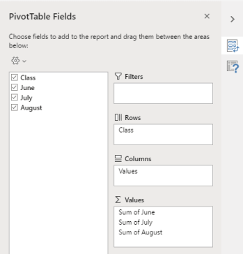
In the PivotTable Fields pane, you can pick the fields you want to show in your PivotTable.
-
In Excel for the web, press F11 to switch to the full screen mode.
-
To move the focus to the PivotTable Fields pane, press Shift+Ctrl+F6 until you hear: «Close button.» The focus is on the Close button in the PivotTable Fields pane.
-
In the PivotTable Fields pane, to move the focus to the list of fields, press the Tab key until you hear the first field in the list. With JAWS and NVDA, you also hear whether the field checkbox is checked or unchecked. With Narrator, to hear if the checkbox is checked or not, press the SR key+Right arrow key repeatedly until Narrator announces the field and the checkbox.
-
To browse the list of fields, use the Down or Up arrow key.
-
When the focus is on a field you want to add to your PivotTable, press Spacebar. The selected field and its data are added to the PivotTable on the worksheet grid. Repeat this step to the fields you want to add to the PivotTable.
The fields you select are added to their default areas: non-numeric fields are added to Rows, date and time hierarchies are added to Columns, and numeric fields are added to Values.
Remove fields from a PivotTable
In the PivotTable Fields pane, you can unselect the fields you don’t want to show in your PivotTable. Removing a field from a PivotTable doesn’t remove the field from the PivotTable Fields pane or delete the source data.
-
In Excel for the web, press F11 to switch to the full screen mode.
-
To move the focus to the PivotTable Fields pane, press Shift+Ctrl+F6 until you hear: «Close button.» The focus is on the Close button in the PivotTable Fields pane.
-
In the PivotTable Fields pane, to move the focus to the list of fields, press the Tab key until you hear the first field in the list. With JAWS and NVDA, you also hear whether the field checkbox is checked or unchecked. With Narrator, to hear if the checkbox is checked or not, press the SR key+Right arrow key until Narrator announces the field and the checkbox.
-
To browse the list of fields, use the Down or Up arrow key.
-
When the focus is on a field you want to remove from your PivotTable, press Spacebar. The field and its data are removed from the PivotTable. Repeat this step to the fields you want to remove from the PivotTable.
Arrange fields in a PivotTable
To rearrange the fields the way you want to display them in the PivotTable, you can move a field from one area to another. You can also move a field up or down within an area.
-
In Excel for the web, press F11 to switch to the full screen mode.
-
To move the focus to the PivotTable Fields pane, press Shift+Ctrl+F6 until you hear: «Close button.» The focus is on the Close button in the PivotTable Fields pane.
-
In the PivotTable Fields pane, press the Tab key until you hear the name of the area that contains the field you want to move, followed by «Has pop-up.» You hear, for example, «Rows,» followed by a field name, and «Has pop-up.»
-
When the focus is on the area you want, press the Down or Up arrow key until you hear the name of the field you want to move.
-
When the focus is on the right field, press Alt+Down arrow key to expand the context menu.
-
Press the Up, Down, Right, or Left arrow key until you hear the option you want, for example, «Move to columns,» and then press Enter. The PivotTable on the worksheet grid is updated accordingly.
The fields in the different areas in the PivotTable Fields pane are shown in the PivotTable as follows:
-
The fields in the Filters area are shown as top-level report filters above the PivotTable.
-
The fields in the Columns area are shown as Column Labels at the top of the PivotTable. Depending on the hierarchy of the fields, columns might be nested inside other columns that are higher in the hierarchy.
-
The fields in the Rows area are shown as Row Labels on the left side of the PivotTable. Depending on the hierarchy of the fields, rows might be nested inside other rows that are higher in the hierarchy.
-
The fields in the Values area are shown as summarized numeric values in the PivotTable.
See also
Use a screen reader to create a PivotTable or PivotChart in Excel
Use a screen reader to filter data in a PivotTable in Excel
Keyboard shortcuts in Excel
Basic tasks using a screen reader with Excel
Use a screen reader to explore and navigate Excel
What’s new in Microsoft 365
Technical support for customers with disabilities
Microsoft wants to provide the best possible experience for all our customers. If you have a disability or questions related to accessibility, please contact the Microsoft Disability Answer Desk for technical assistance. The Disability Answer Desk support team is trained in using many popular assistive technologies and can offer assistance in English, Spanish, French, and American Sign Language. Please go to the Microsoft Disability Answer Desk site to find out the contact details for your region.
If you are a government, commercial, or enterprise user, please contact the enterprise Disability Answer Desk.
Need more help?
Want more options?
Explore subscription benefits, browse training courses, learn how to secure your device, and more.
Communities help you ask and answer questions, give feedback, and hear from experts with rich knowledge.
Find solutions to common problems or get help from a support agent.
When just starting out people often find themselves wondering how to add a whole column in Excel. Usually, a formula only applies to a range of cells, not the entire column.
This is actually really simple to achieve and I will show you two quick methods on how to do it: one with a formula, the other using Excel’s Status bar.
How to add an entire column in Excel using a formula
- Select the cell where you want to insert the sum
- Type =SUM(
- Select the entire column by clicking on the column letter
- Type ) to finish the formula and hit Enter
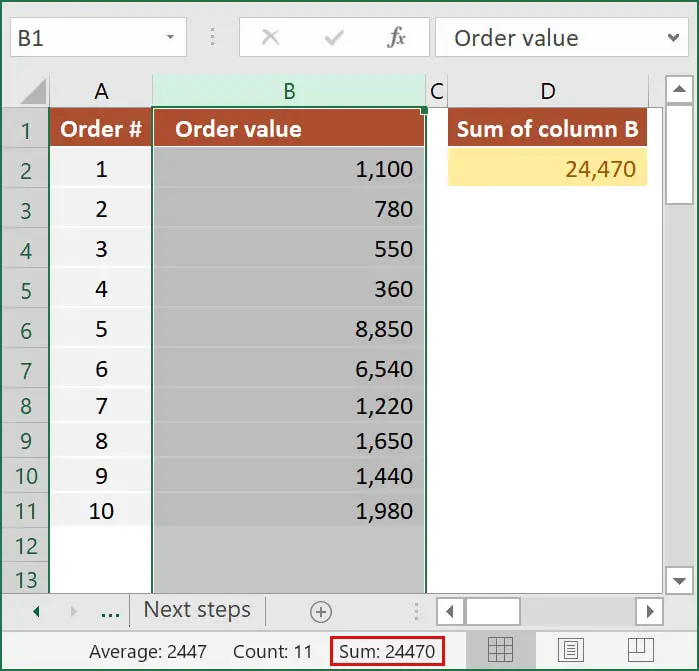
In the example shown, the formula in D2 is =SUM(B:B). This sums up all values from column B.

If you need additional info, I also wrote an article on how to use SUM function in Excel.
How to add a column of numbers in Excel using the Status bar
The second option is to use the Status bar. This is useful when you just want a quick glance at the total sum of values, rather than actually calculating the sum using a formula.
- Select the entire column by clicking on the column letter
- Check the Sum field from the Status bar
Note: Be careful when referencing an entire column. While it may be useful to include all values in your formulas, this approach is prone to errors. If you accidentally insert a value anywhere in that column, it will be added to your result.
I hope this article showed you exactly how to add a whole column in Excel. However, in case you still have questions, don’t hesitate to reach out.
Skip to content
![]()
After you create a pivot table, you can add or remove fields by using the check boxes in the field list. Text fields are automatically added to the Row Labels area, and numeric fields go into the Values area.

Once the fields are in the layout, you can drag them to a different location, by using the layout boxes in the field list. In the next screen shot, the Region field is being moved from the Rows area to the Filters area.

Add All Remaining Fields
If there are only a few fields in the pivot table, it’s easy to check the boxes and add them all manually. You have to do these one at a time though — there isn’t a “Select All” checkbox. If there is a long list of fields, you could manually add a few, and then use a macro to put the rest in the Row Labels area, or the Values area.
In the following code, all the remaining fields are added to the Values area. There is another sample on my Contextures site, that adds all the remaining fields to the Row Labels area.
Put this code in a regular code module. Then select a cell in the pivot table that you want to update, and run the macro.
Sub AddAllFieldsValues()
Dim pt As PivotTable
Dim iCol As Long
Dim iColEnd As Long

Set pt = ActiveSheet.PivotTables(1)

With pt
   iCol = 1
   iColEnd = .PivotFields.Count

    For iCol = 1 To iColEnd
        With .PivotFields(iCol)
          If .Orientation = 0 Then
              .Orientation = xlDataField
          End If
        End With
    Next iCol
End With

End Sub
______________________
Transcript
Once you’ve created a pivot table, you need to add fields to it in order for it to be useful. The fields in a pivot table correspond to columns in the source data.
Let’s take a look.
Here we have a set of data that’s already formatted as an Excel Table. Let’s use this table to create a pivot table and add some fields. Since the source data is already a Table, we’ll use the Summarize With Pivot Table command, on the Table Tools Design tab.
Let’s accept the defaults, and let Excel create the pivot table on a new worksheet. A new pivot table doesn’t have any fields, so our first task is to add some.
The easiest way to add a field to a pivot table is to check the box next to the field you want to add.
By default, fields that contain numeric information are added to the Values area of the pivot table, and fields that contain text are added to the row label area.
Fields added to the Row Labels area appear as labels at the left of the table, and fields added to the Column Labels area appear as headings across the top of the table. Fields added to the Values area appear inside the table.
You can see how the field list pane mimics the pivot table layout.
To remove a field, just uncheck the box. Or, simply drag the field out of the field list pane. You can also click the field drop-down menu and select Remove Field from the menu.
Another way to add a field to a pivot table is to drag it from the field list into the location you like below.
Finally, you can add a field by right-clicking. Right-click and choose a location from the menu.
If you ever want to reset a pivot table back to its original blank state, it’s easy to do. Just click a cell in the pivot table, and click the Clear menu, on the Options tab of the PivotTable Tools ribbon. Then select Clear All. All fields will be removed from the pivot table at once.
Adding a column in Excel means inserting a new column to the existing dataset. Besides inserting, one may need to delete, hide, unhide, and move rows or columns. Such modifications help in structuring and organizing the dataset. As a result, it is essential to be aware of the techniques related to these alterations.
For example, while preparing a consolidated balance sheet, Mr. X realizes that the data related to the previous year is missing. To include this data, he wants to insert a new column. Here, the method of inserting a column comes into use.
Excel provides different ways of performing actions on a dataset. This article discusses the most appropriate and effective methods of working with data. It covers the following aspects: –
- Insert Excel columns (alternate methods and shortcuts)
- Delete columns and rows
- Hide and unhide rows or columns
- Move rows or columns
Apart from inserting columns in Excel, the remaining topics have been covered in brief.
Table of contents
- How to Add/Insert Columns in Excel?
- Example #1–Add Columns in Excel
- Example #2–Alternate Method to Insert Rows and Columns in Excel
- Example #3–Hide and Unhide Columns & Rows in Excel
- Example #4–Move Rows or Columns in Excel
- Shortcuts to Insert Columns in Excel
- Frequently Asked Questions
- Recommended Articles
How to Add/Insert Columns in Excel?
Below are some examples through which you may learn how to add and insert columns in Excel.
Example #1–Add Columns in Excel
The following table shows the first and the last names in columns A and B, respectively. We want to insert a new column (column B) between these names, which will display the middle name.

The steps to insert a new column (column B) between two existing columns (columns A and B) are listed as follows:
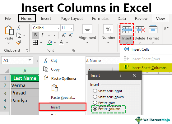
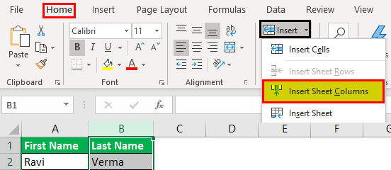
Step 1: Select any cell of column B. Alternatively, one can also select column B, as shown in the following image. Further, click the “Insert” drop-down from the “Home” tab of the Excel ribbonThe ribbon is an element of the UI (User Interface) which is seen as a strip that consists of buttons or tabs; it is available at the top of the excel sheet. This option was first introduced in the Microsoft Excel 2007.read more. Finally, select “Insert Sheet Columns.”
Note: To select a column, click its label or header on top.
Step 2: A new column (column B) is inserted between the columns containing the first and the last names. As a result, the data (last name) of the previous column B (shown in step 1) now shifts to column C.
Note: Excel inserts a column immediately preceding the column of the selected cell. Hence, one must always choose a cell accordingly. If a column is selected, Excel inserts a column preceding it.

Example #2–Alternate Method to Insert Rows and Columns in Excel
Working on the data of example #1, we need to insert a middle name column using the following methods:
a) Select and right-click a cell
b) Select and right-click a column
a) The steps for inserting a column after selecting and right-clicking a cell are listed as follows:
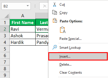
Step 1: Select any cell of column B. This is because a column preceding column B is to be inserted. Right-click the selection and choose “insert,” as shown in the following image.
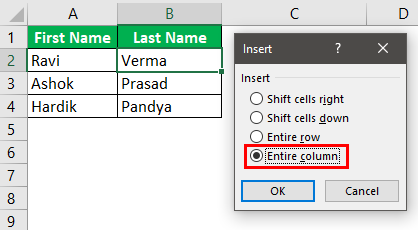
Step 2: The “Insert” dialog box appears. Select “Entire column” to insert a new column.
Note: For inserting a new row, select “Entire row.”
Step 3: A new column (column B) for typing middle names has been inserted.

b) The steps for inserting a column after selecting and right-clicking a column are listed as follows:
Step 1: Select the entire column B. That is because a column preceding column B is to be inserted. Right-click the selection and choose “Insert,” as shown in the following image.
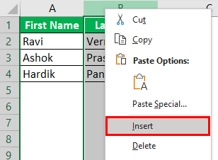
Step 2: A new column B is inserted. The same has been shown under step 3 of method a.
Note: Select the entire row preceding which a new row is inserted for inserting rows. Right-click the selection and choose “Insert.” The same is shown in the following image.

Example #3–Hide and Unhide Columns & Rows in Excel
Working on the data of example #1, we want to perform the following tasks:
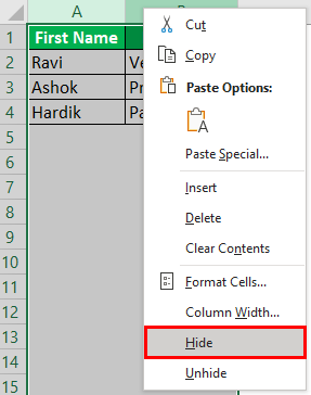
a) Hide columns A and B or rows 3 and 4 by right-clicking
b) Hide column A by using the “format” drop-down
c) Unhide columns B and C by right-clicking
a) The steps to hide the columns A and B or rows 3 and 4 by right-clicking are listed as follows:
Step 1: Select columns A and B. Right-click the selection and choose “hide,” as shown in the next image.
Note 1: To select a row or column, click the row number (to the left) or the column label (on top).
Note 2: Multiple adjacent rows or columns can be selected by dragging across the row and column headings. Alternatively, hold the “Shift” key while selecting the rows or columns.
Note 3: We can select non-adjacent rows or columns by holding the “Ctrl” key while making the selections.
Step 2: Columns A and B will be hidden. Likewise, select rows 3 and 4. Right-click the selection and choose the “Hide” option from the context menu. The same is shown in the following image.
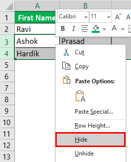
It will hide rows 3 and 4.
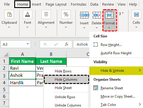
b) The steps to hide column A by using the “format” drop-down are listed as follows:
Step 1: Select any cell of column A. Click the “Format” drop-down under the “Home” tab of the Excel ribbon. Next, select “Hide Columns” under the “Hide & Unhide” option.
The same is shown in the following image.
Note: Alternatively, select the relevant column to be hidden. Click “Hide columns” under the “Hide & Unhide” option.
Step 2: We will hide the column of the selected cell, column A. Likewise, to hide rows, select the relevant row. Then, choose “Hide Rows” from the “Hide & Unhide” option of the “Format” drop-down.
c) The steps to unhide columns B and C by right-clicking are listed as follows:
Step 1: Select the unhidden columns (A and D) immediately before and after the hidden columns (B and C). Right-click the selection and choose “Unhide.”
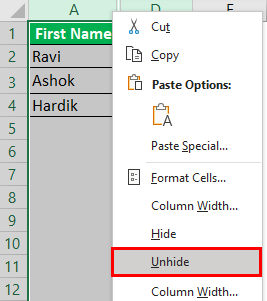
Step 2: The columns B and C will be unhidden. The dataset appears as shown in step 1 of task b.
Likewise, unhide rows by selecting the “Unhide rows” (immediately before and after the hidden rows) and clicking “Unhide” from the context menu.
Example #4–Move Rows or Columns in Excel
Working on the data of example #1, we want to move column B (last name) to precede column A (first name).
The steps to move column B are listed as follows:
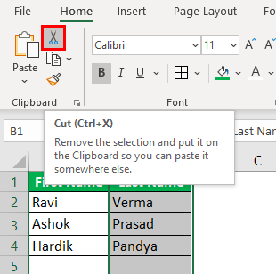
Step 1: Select column B, which is to be moved. Cut it in either of the following ways:
- Press “Ctrl+X.”
- Click the scissors icon from the “Clipboard” group of the “Home” tab.
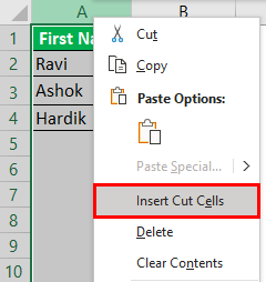
Step 2: Select column A, where the data of column B is to be pasted. Right-click the selection and choose “Insert Cut Cells.”
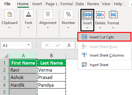
Alternatively, select “Insert Cut Cells” from the “Insert” drop-down of the “Home” tab. The same is shown in the following image.
Note: The “Insert Cut Cells” option will be visible once the selected cells have been cut.
Step 3: The data of column B is pasted into column A. Hence, the first column (column A) now contains the last names. The data of the initial column A (first name) automatically shifts to column B.
The same is shown in the following image.
Note: A row can be selected, cut, and pasted to the desired location. Select the “Insert Cut Cells” option from the “Insert” drop-down of the “Home” tab for pasting.

Shortcuts to Insert Columns in Excel
Let us go through the two shortcuts for inserting columns and rows.
a) Shortcut for inserting with the “Insert” drop-down of the “Home” tab
The excel shortcutAn Excel shortcut is a technique of performing a manual task in a quicker way.read more for inserting a row or column with the “Insert” drop-down works as follows:
- Select a cell preceding which a row or column is inserted.
- Click the “Insert” drop-down from the “Cells” group of the “Home” tab.
- Press “R” to insert a row or “C” to insert a column
A new row or column is inserted depending on the third pointer’s key.
Note: Under the “Insert” drop-down, the “R” of “insert sheet rows” and the “C” of “insert sheet columns” are underlined. Hence, these keys work as shortcuts for inserting rows and columns.
b) Shortcut for inserting with right-click
- The shortcut for inserting a row or column with right-click works as follows:
- Select a cell preceding which a row or column is inserted.
- Right-click the selection and press “I.” The “Insert” dialog box opens.
- Press “R” to insert a row or “C” to insert a column.
- Press the “Enter” key.
A new row or column is inserted depending on the third pointer’s key.
Note: If the “Insert” dialog box does not open in step 2, press the “Enter” key after pressing “I.” It opens the “Insert” dialog box.
Frequently Asked Questions
1. What does it mean to insert a column? How is it done in Excel?
Inserting a column refers to adding a new column to an existing dataset. This new column may contain additional data that can be important for the end-user.
Additionally, there is a possibility that a column has been omitted by mistake. In such cases, inserting a column will be helpful.
The steps to insert a column in Excel are listed as follows:
a. Select the column preceding which a new column is to be inserted.
b. Right-click the selection and choose “Insert” from the context menu.
It will insert the new column immediately before the selected column.
Note: To select a column, click its header (label) on top.
2. How to insert a column in Excel by using a shortcut?
Let us insert a new column E in Excel. The steps to insert a column (column E) by using a shortcut are listed as follows:
a. Select the existing column E.
b. Press the keys “Ctrl+Shift+plus sign(+)” together to insert a column.
It will insert the new column E. The data of the initial column E now shifts to column F.
Note 1: One must select a column carefully. That is because Excel inserts a column preceding the selected column.
Note 2: As an alternative to step a, one can select any cell of column E. After that, press “Ctrl+space” to select the entire column E.
3. How to insert multiple adjacent columns in Excel?
Let us insert columns D, E, and F in Excel. The steps to insert multiple columns (D, E, and F) are listed as follows:
a. Select as many columns in the existing dataset as the number of the new columns to be inserted. So, select the current columns D, E, and F.
b. Press the keys “Ctrl+Shift+plus sign(+)” together.
It will insert the blank columns D, E, and F. The initial columns D, E, and F data shift to columns G, H, and I.
Note 1: Alternative to step a: select adjacent cells of columns D, E, and F. These cells should be in one row. Further, press “Ctrl+space.” As a result, columns D, E, and F will be selected.
Note 2: To select multiple adjacent columns (in step a), drag across the column headings. Alternatively, hold the “Shift” key while selecting the columns.
Note 3: Alternative to step b: right-click the selection and choose “Insert.”
Recommended Articles
This article is a guide to Add Columns in Excel. We also discuss inserting, hiding, and moving rows and columns in Excel and practical examples. You may learn more about Excel from the following articles: –
- Compare Two Columns in Excel for Matches
- 3 Ways to Show Excel Negative Numbers
- Rows vs. Columns
- Move Columns in Excel
I would like to add every field that I select as a value (instead they are automatically added as rows) and as a product (they are automatically a count).
This would save me a massive amount of time. So far I have not found any default add options.
Any help would be greatly appreciated.
Thanks.
asked Oct 1, 2014 at 19:56
![]()
This has been a problem with Excel for a long time. The solution to your first problem is to drag the fields into the value field box under the field list.
There is no way to change the default summary operation, but the reason you’re getting COUNT is that there are some cells in the data that contain non-numeric values (otherwise you’d get SUM.)
The only solution I’ve seen for this is to program your own pivot table builder in VBA or write a macro that automatically updates all fields in the table to a certain operation after they are added.
answered Oct 1, 2014 at 20:05
![]()
Mr. MascaroMr. Mascaro
2,6931 gold badge11 silver badges18 bronze badges
3
To convert from count to Sum, i found the below works for me.
-
Click any cell in your pivot table.
-
Hold down the ALT + F11 keys, and it opens the Microsoft Visual Basic for Applications window.
-
Click Insert > Module, and paste the following code in the Module Window.
VBA code: Change multiple field settings in pivot table
Public Sub SetDataFieldsToSum()
    'Update 20141127
    Dim xPF As PivotField
    Dim WorkRng As Range
    Set WorkRng = Application.Selection
    With WorkRng.PivotTable
       .ManualUpdate = True
       For Each xPF In .DataFields
          With xPF
             .Function = xlSum
             .NumberFormat = "#,##0"
          End With
       Next
       .ManualUpdate = False
    End With
End Sub
- Then press F5 key to execute this code, and all the field settings in your selected pivot table have been converted to your need calculation at once
![]()
answered Aug 6, 2019 at 6:55
![]()
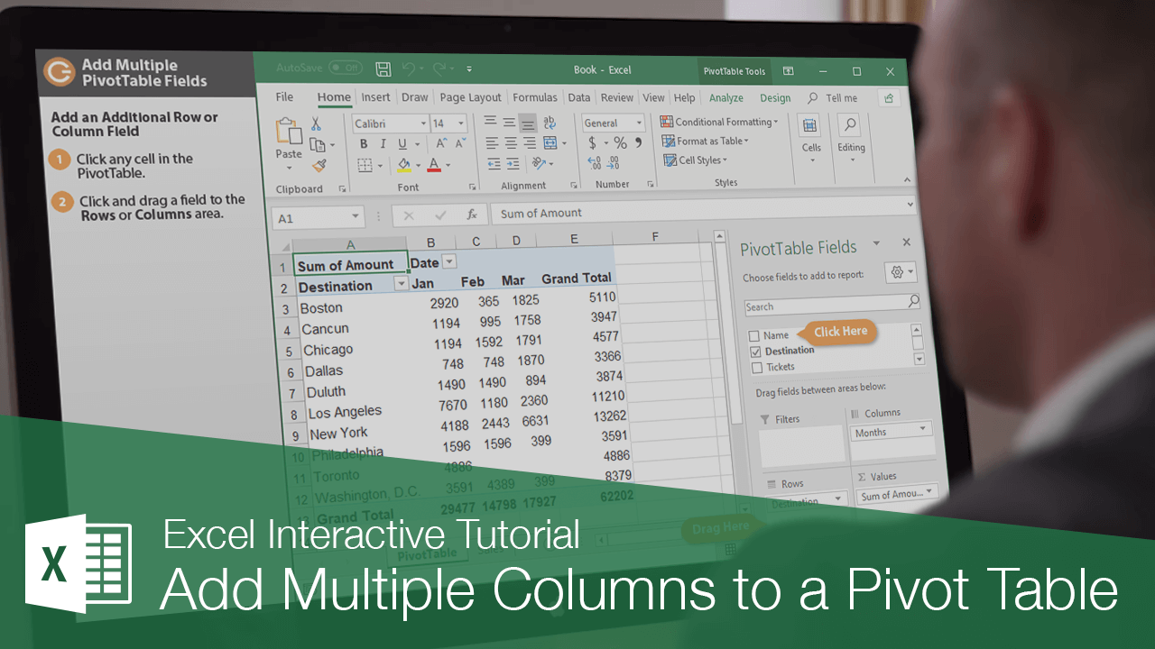
When adding fields to the Filters, Columns, Rows, and Values areas of a PivotTable, you aren’t limited to just adding one field; you can add as many as you like. However, if you make it too complex, the PivotTable will start to become difficult to consume. You may need to experiment with adding multiple fields to certain areas to see what works best for your set of data. Remember, you can always drag fields out of the area you’ve added them to in the PivotTable Fields pane to remove them.
Let’s refer back to our previous example, where we are only interested in seeing the monthly sales for each destination. After creating the PivotTable, your boss may request to see data for which agents made those sales. Instead of creating a separate PivotTable, you can easily add the Name field as an additional row to expand the data that’s represented.
Add an Additional Row or Column Field
- Click any cell in the PivotTable.
The PivotTable Fields pane appears.
You can also turn on the PivotTable Fields pane by clicking the Field List button on the Analyze tab.
- Click and drag a field to the Rows or Columns area.

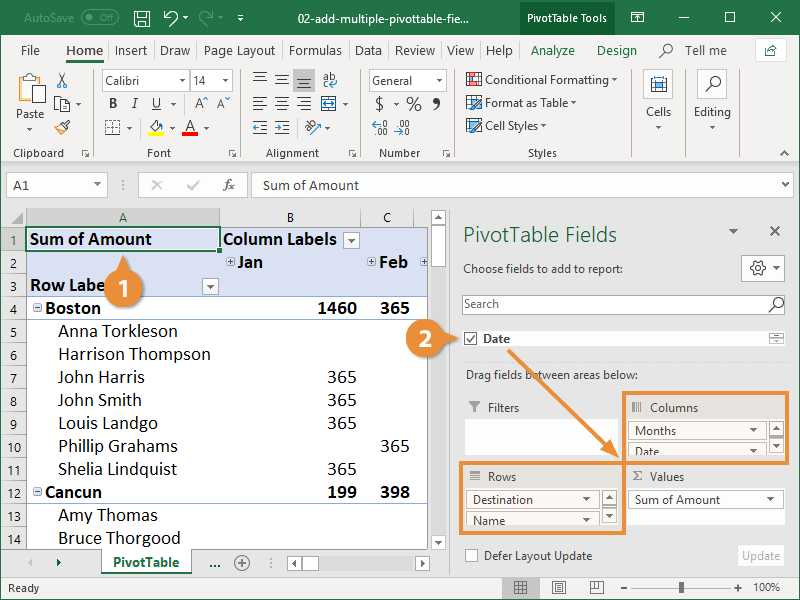
The PivotTable is updated to include the additional values. The order you place the fields in each area in the Fields pane affects the look of the PivotTable. You can drag the field values up or down within an area (the Rows area, for example) to adjust which data appears first.
Some fields, when added to a PivotTable, will automatically be displayed as two fields. For example, when adding a date field to the Columns area, Excel will likely group the dates into months automatically instead of displaying each individual date as a column heading. In the Columns area of the PivotTable Fields pane, you’ll see two fields—Date and Months—even though you only added a single field.
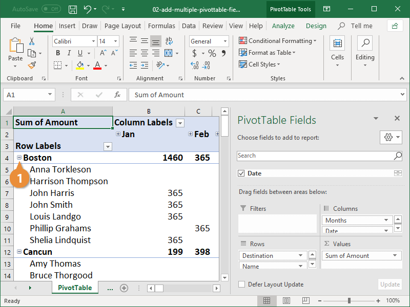
Expand or Collapse a Heading
Once you’ve added more than one value to an area, expand and collapse buttons appear for the top-level values in the PivotTable. Use these to change how much of the data is visible at once.
- Click the Expand or Collapse symbol next to a row or column heading.
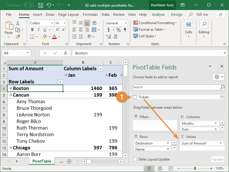
Add an Additional Value Field
If your original set of data has multiple columns with numeric values, you may find yourself adding additional fields to the Values area. If this is the case, the PivotTable will display the sum of one set of data followed by the sum of the second set of data in an adjacent column.
- Click and drag a second field to the Values area.
The order in which you place the fields in the Values area is very important. If you add a field and the PivotTable doesn’t look right, try adjusting the order of the fields until the PivotTable displays useful data.

FREE Quick Reference
Click to Download
Free to distribute with our compliments; we hope you will consider our paid training.

Excel Add Column (Table of Contents)
- Add Column in Excel
- How to Add Column in Excel?
- How to Modify a Column Width?
Add Column in Excel
Excel allows a user to add columns, whether left or right, of the column in the worksheet, which is called Add Column in Excel. Of course, there is more than one way to accomplish a task, as in all Microsoft programs. These instructions cover how rows and columns can be added and modified in an Excel worksheet using a keyboard shortcut and using the context menu with the right-click.
How to Add Column in Excel?
Adding a column in Excel is very easy and convenient whenever we want to add data to the table. There are different Methods to Insert or add Column which is as follows:
- Manually we can do this by just right-clicking on the selected column> then click on the insert button.
- Use Shift + Ctrl + + shortcut to add a new column in the Excel.
- Home tab >> click on Insert >> Select Insert Sheet Columns.
- We can add N number of columns in the Excel sheet; a user needs to select that many columns which number of columns he wants to insert.
Let’s understand How to Add Column in Excel with a few examples.
Example #1
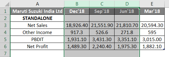
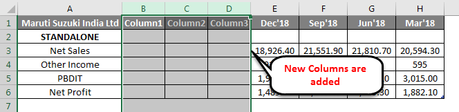
A user has a standalone book data of sales, income, PBDIT, and Profit details of each quarter of Maruti Suzuki India Pvt Ltd in sheet1.
You can download this Add a Column Excel Template here – Add a Column Excel Template
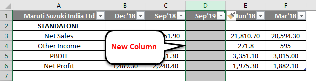
Step 1: Select the column where a user wants to add the column in the excel worksheet (The new column will be inserted to the left of the selected column, so select accordingly)
Step 2: A user has selected the D column where he wants to insert the new column.
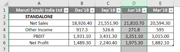
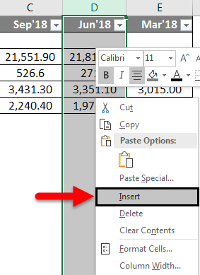
Step 3: Now Right-click and select Insert button or use shortcut Shift + Ctrl + +
Or

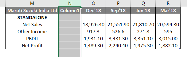
As we can see, as it was required to insert a new column between C and D column, in the above example, we have added a new column. So, as a result, it will move the D column data to the next column, which is E, and it will take the place of D.
Example #2
Let’s take the same data to analyze this example. A user wants to insert three columns left of the B column.
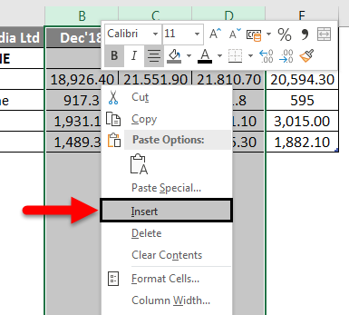
Step 1: Select B, C, and D columns where a user wants to insert new 3 columns in the worksheet (The new column is inserted to the left of the selected column, so select accordingly)
Step 2: A user has selected the B, C, and D columns where he wants to insert a new column
Step 3: Now Right-click and select Insert button or use shortcut Shift + Ctrl + +
Or
As we can see, as it was required to insert a new column left of the B, C, and D column, we added a new column in the above example. As a result, it will move B, C, and D column data to the next column, which are E, F, and G; it will take the place of the B, C, and D column.
Example #3
Step 1: Go to Worksheet >> Select the column’s heading where a user wants to insert a new column.
Step 2: Click on the Insert button.
Step 3: One drop-down will be open; click on the Insert Sheet Columns.
As the user wants to use the Insert toolbar to insert a new column, as in the above example, it added.
Example #4
The user can insert a new column in any version of Excel; in the above examples, we can see that we had selected one or more columns in the worksheet then >Right click on the selected column> then clicked on the Insert button.
To add a new column in the excel worksheet.
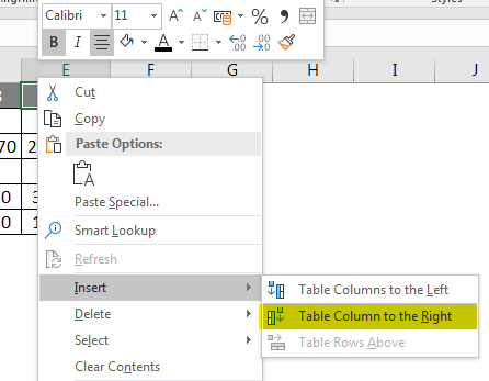
Click in a cell to the left or right of where you want to add a column. If the user wants to add a column to the left of the cell, then follow the below process:
- Click on Table Columns to the Left from the Insert option.
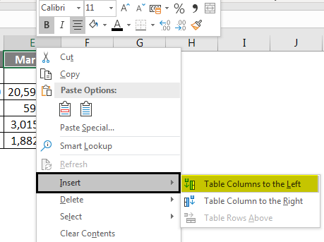
And if a user wants to insert the column to the right of the cell, then follow the below process:
- Click on Table Columns to the Right from the Insert option.
How to Modify a Column Width?
A user can modify the width of any column. Let’s take an example as some of the content in column A cannot be displayed. We can make all this content visible by changing the width of column A.
Step 1: Position the mouse over the column line in the column heading to the Black Cross. (As shown below)
Step 2: Click, hold and drag the mouse to increase or decrease the column width.
Step 3: Release the mouse. The column width will be changed.
A user can auto fit the width of the column. The AutoFit feature will allow you to set a column’s width to fit its content automatically.
Step1: Position the mouse over the column line in the column heading to the Black Cross.
Step2: Double-click the mouse. The column width will be changed automatically to fit the content.
Things to Remember About Add a Column in Excel
- The user needs to select that column where the user wants to insert the new column.
- By default, every row and column have the same height and width, but a user can modify the width of the column and the height of the row.
- The user can insert multiple columns at a time.
- You can also AutoFit the width for several columns at the same time. Simply select the columns you want to AutoFit, and then select the AutoFit Column Width command from the Format drop-down menu on the Home. This method can also be used for row height.
- All the rules will also be applied for rows, as applied to column insertion.
- Excel allows the user to wrap text and merging cells.
- For deleting also, we can go to Home Tab >> Delete >> Delete Sheet Columns; either we can select the column which we want to delete or >> Right Click >> click on Delete.
- After adding the insert column, all the data will be shifted to the right side after that column.
Recommended Articles
This is a guide to add a column in excel. Here we have discussed How to Add a column in excel by using different methods and How to modify a column in Excel along with practical examples and a downloadable excel template. You can also go through our other suggested articles –
- COLUMNS Formula in Excel
- Switching Columns in Excel
- Excel COLUMN to Number
- Freeze Columns in Excel
Data entry can sometimes be a big part of using Excel.
With near endless cells, it can be hard for the person inputting data to know where to put what data.
A data entry form can solve this problem and help guide the user to input the correct data in the correct place.
Excel has had VBA user forms for a long time, but they are complicated to set up and not very flexible to change.
In this blog post, we’re going to explore 5 easy ways to create a data entry form for Excel.
Video Tutorial
Excel Tables
We’ve had Excel tables since Excel 2007.
They’re perfect data containers and can be used as a simple data entry form.
Creating a table is easy.
- Select the range of data including the column headings.
- Go to the Insert tab in the ribbon.
- Press the Table button in the Tables section.
We can also use a keyboard shortcut to create a table. The Ctrl + T keyboard shortcut will do the same thing.
Make sure the Create Table dialog box has the My table has headers option checked and press the OK button.
We now have our data inside an Excel table and we can use this to enter new data.
To add new data into our table we can start typing a new entry into the cells directly below the table and the table will absorb the new data.
We can use the Tab key instead of Enter while entering our data. This will cause the active cell cursor to move to the right instead of down so we can add the next value into our record.
When the active cell cursor is in the last cell of the table (lower right cell), pressing the Tab key will create a new empty row in the table ready for the next entry.
This is a perfect and simple data entry form.
Data Entry Form
Excel actually has a hidden data entry form and we can access it by adding the command to the Quick Access Toolbar.
Add the form command to the Quick Access Toolbar.
- Right click anywhere on the quick quick access toolbar.
- Select Customize Quick Access Toolbar from the menu options.
This will open up the Excel option menu on the Quick Access Toolbar tab.
- Select Commands Not in the Ribbon.
- Select Form from the list of available commands. Press F to jump to the commands starting with F.
- Press the Add button to add the command into the quick access toolbar.
- Press the OK button.
We can then open up data entry form for any set of data.
- Select a cell inside the data which we want to create a data entry form with.
- Click on the Form icon in the quick access toolbar area.
This will open up a customized data entry form based on the fields in our data.
Microsoft Forms
If we need a simple data entry form, why not use Microsoft Forms?
This form option will require our Excel workbook to be saved into SharePoint or OneDrive.
The form will be in a browser and not in Excel, but we can link the form to an Excel workbook so that all the data goes into our Excel table.
This is a great option if multiple people or people outside our organization need to input data into the Excel workbook.
We need to create a Form for Excel in either SharePoint or OneDrive. The process is the same for both SharePoint or OneDrive.
- Go to a SharePoint document library or a OneDrive folder where the Excel workbook is going to be saved.
- Click on New and then choose Forms for Excel.
This will prompt us to name the Excel workbook and open up a new browser tab where we can build our form by adding different types of questions.
We first need to create the Form and this will create the table in our Excel workbook where the data will get populated.
Then we can share the form with anyone we want to input data into Excel.
When a user enters data into the form and presses the submit button, that data will automatically show up into our Excel workbook.
Power Apps
Power Apps is a flexible drag and drop formula based app building platform from Microsoft.
We can certainly use it to create a data entry from for our Excel data.
In fact, if we have a table of data set up, Power Apps will create the app for us based on our data. It can’t be any easier than that.
Sign in to the powerapps.microsoft.com service ➜ go to the Create tab in the navigation pane ➜ select Excel Online.
We’ll then be prompted to sign in to our SharePoint or OneDrive account where our Excel file is saved to select the Excel workbook and table with our data.
This will generate us a fully functional three screen data entry app.
- We can search and view all the records in our Excel table in a scroll-able gallery.
- We can view an individual record in our data.
- We can edit an existing record or add new records.
This is all connected to our Excel table, so any changes or additions from the app will show up in Excel.
Power Automate
Power Automate is a cloud based tool for automating task between apps.
But we can use the button trigger to make an automation that captures user input and adds the data into an Excel table.
We’ll need to have our Excel workbook saved in OneDrive or SharePoint and have a table already setup with the fields we want to populate.
To create our Power Automate data entry form.
- Go to flow.microsoft.com and sign in.
- Go to the Create tab.
- Create an Instant flow.
- Give the flow a name.
- Choose the Manually trigger a flow option as the trigger.
- Press the Create button.
This will open up the Power Automate builder and we can build our automation.
- Click on the Manually trigger a flow block to expand the trigger’s options. This is where we’ll find the ability to add input fields.
- Click on the Add an input button. This will give us options to add a few different types of input fields including Text, Yes/No, Files, Email, Number and Dates.
- Rename the field to something descriptive. This will help the user know what type of data to input when they run this automation.
- Click on the three ellipses to the right of each field to change the input options. We’ll be able to Add a drop-down list of option, Add a multi-select list of options, Make the field optional or Delete the field from this menu.
- After we have added all our input fields, we can now add a New step to the automation.
Search for the Excel connector and add the Add a row into a table action. If you’re on an Office 365 business account, use the Excel Online (Business) connectors, otherwise use the Excel Online (OneDrive) connectors.
Now we can set up our Excel Add a row into a table step.
- Navigate to the Excel file and table where we are going to be adding data.
- After selecting the table, the fields in that table will appear listed and we can add the appropriate dynamic content from the Manually trigger a flow trigger step.
Now we can run our Flow from the Power Automate service.
- Go to My flows in the left navigation pane.
- Go to the My flows tab.
- Find the flow in the list of available flows and click on the Run button.
- A side pane will pop up with our inputs and we can enter our data.
- Click Run flow.
We can also run this from our mobile device with the Power Automate apps.
- Go to the Buttons section in the app.
- Press on the flow to run.
- Enter the data inputs in the form.
- Press on the DONE button in the top right.
Whichever way we run the flow, a few seconds later the data will appear in our Excel table.
Conclusions
Whether we require a simple form or something more complex and customize-able, there is a solution for our data entry needs.
We can quickly create something inside our workbook or use an external solution that connects to and loads data into Excel.
We can even create forms that people outside our organization can use to populate our spreadsheets.
Let me know in the comments what is your favourite data entry form option.
About the Author
John is a Microsoft MVP and qualified actuary with over 15 years of experience. He has worked in a variety of industries, including insurance, ad tech, and most recently Power Platform consulting. He is a keen problem solver and has a passion for using technology to make businesses more efficient.