Add a value to all cells in excel

One quick and easy way to add values in Excel is to use AutoSum. Just select an empty cell directly below a column of data. Then on the Formula tab, click AutoSum > Sum. Excel will automatically sense the range to be summed. (AutoSum can also work horizontally if you select an empty cell to the right of the cells to be summed.)

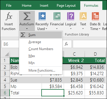
AutoSum creates the formula for you, so that you don’t have to do the typing. However, if you prefer typing the formula yourself, see the SUM function. 

Add based on conditions

• Use the SUMIF function when you want to sum values with one condition. For example, when you need to add up the total sales of a certain product.

• Use the SUMIFS function when you want to sum values with more than one condition. For instance, you might want to add up the total sales of a certain product, within a certain sales region.

Add or subtract dates

For an overview of how to add or subtract dates, see Add or subtract dates. For more complex date calculations, see Date and time functions.

Add or subtract time

For an overview of how to add or subtract time, see Add or subtract time. For other time calculations, see Date and time functions.

Need more help?

You can always ask an expert in the Excel Tech Community or get support in the Answers community.

See all How-To Articles

This tutorial demonstrates how to add values to cells and columns in Excel and Google Sheets.

Add Values to Multiple Cells

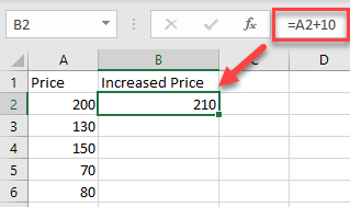
1. To add a value to a range of cells, click on the cell where you want to display the result, and enter = (equal) and the cell reference of the first number then + (plus) and the number you want to add.

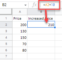
For this example, start with cell A2 (200). Cell B2 will show the Price in A2 increased by 10. So, in cell B2, enter:

=A2+10

As a result, the value in cell B2 is now 210 (value from A2 plus 10).

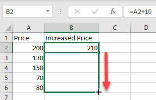
1. Now copy this formula down the column to the rows below. Click on the cell where you entered the formula (F2) and place your cursor on the bottom right corner of the cell.
2. When it changes to a plus sign, drag it down to the rest of the rows where you want to apply the formula (here, B2:B6).

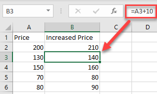
As a result of relative cell referencing, the constant (here, 10) remains the same, but the cell address changes according to the row you are in (so B3=A3+10, and so on).

Add Multiple Cells With Paste Special

You can also add a number to multiple cells and return the result as a number in the same cell.

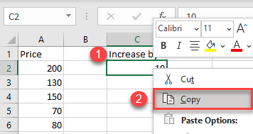
1. First, select the cell with the value you want to add (here, cell C2), right-click, and from the drop-down menu, choose Copy (or use the shortcut CTRL + C).

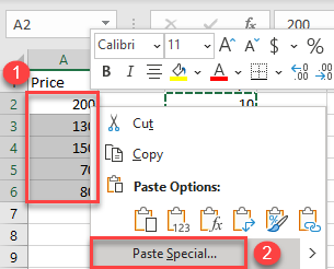
1. After that, select the cells where you want to subtract the value and right-click on the data range (here, A2:A6). In the drop-down menu, click on Paste Special.

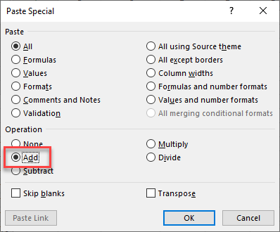
1. The Paste Special window will appear. Under the Operation section choose Add, and then click OK.

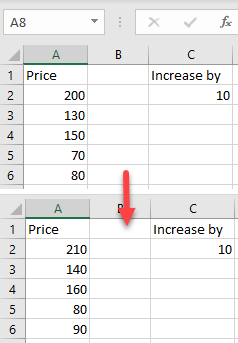
You’ll see the result as a number within the same cells. (In this example, 10 was added to each value from the data range A2:A6.) This method is better if you don’t want to display the results in a new column and don’t need to retain a record of the original values.

Add Column With Cell References

To add an entire column to another using cell references, select the cell where you want to display the result, and enter = (equal) and the cell reference for the first number then + (plus) and the reference for the cell you want to add.

For this example, calculate the summary of Price 1 (A2) and Price 2 (B2). So, in cell C2, enter:

=A2+B2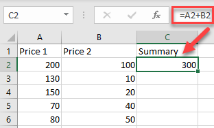

To apply the formula to an entire column, just copy the formula down to the rest of the rows in the table (here, C2:C6).

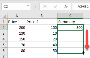
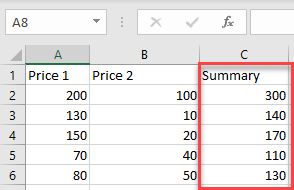
Now, you have a new column with the summary.

Using the methods above, you can also subtract, multiply, or divide cells and columns in Excel.

Add Cells and Columns in Google Sheets

In Google Sheets, you can add multiple cells using formulas in exactly the same ways as in Excel; except, you can’t use Paste Special.

This is addition to @Edward-Leno ‘s answer for more detail/explanation and cases where the text cells are formulas instead of values, and you want to retain the original formula.

Suppose your cells look like this (formulas)

=»email» & «@» & «address.com»

=A1 & «@» & C1

instead of this (values)

email@address.com

If «email» and «address.com» were some cells like A1 is the email and C1 is the address.com part, then you’d have something like =A1&»@»&C1 which would be important to retain since A1 and C1 might not be constants and can change, so the comma-concatenated values would change, like if C1 is «gmail.com», «yahoo.com», or something else based on its formula.

Values method: The following steps will successfully append text but only keep the value using a scratch column (this works for rows, too, but for simplicity, the directions are for columns)

1. Assume column A is your data.
2. In scratch column B, start anywhere like the top of column B such as at B1 and put this formula:

=A1&»,»

Essentially, the «&» is the concatenation operator, combining two strings together (numbers are converted to strings). The «,» can be adjusted to «, » if you want a space after the comma.

1. Copy the cell B1 and copy it down to all other cells in column B, either by clicking at the bottom right of cell B1 and dragging down, or copying with «Ctrl+C» or right-click > «Copy».

2. Paste B1 to all cells in column B with «Ctrl+V» or right-click > «Paste Options:» > «Paste». You should see the data looking like you intended.

3. Copy all cells in column B and paste them to where you want via right-click > «Paste Options:» > «Values». We select values so it doesn’t mess up any formatting or conditional formatting

Formula retention method: The following steps will successfully retain the original formula. The process is similar to the values method, and only step 2, the formula used to concatenate the comma, changes.

1. Assume column A is your data.
2. In scratch column B, start anywhere like the top of column B such as at B1 and put this formula:

=FORMULATEXT(A1)&»,»

FORMULATEXT() grabs the formula of the cell as opposed to the value of it, so a simple example would be that it grabs =2+2 instead of 4, or =A1 & «@» & C1 where A1 is «Bob» and C1 is «gmail.com» instead of Bob@gmail.com.

Note: This formula only works for Excel versions 2013 and greater. For alternative equivalent solutions for Excel 2010 and older, see this superuser answer: https://superuser.com/a/894441/495155

1. Copy the cell B1 and copy it down to all other cells in column B, either by clicking at the bottom right of cell B1 and dragging down, or copying with «Ctrl+C» or right-click > «Copy».

2. Paste B1 to all cells in column B with «Ctrl+V» or right-click > «Paste Options:» > «Paste». You should see the data looking like you intended.

3. Copy all cells in column B and paste them to where you want via right-click > «Paste Options:» > «Values». We select values so it doesn’t mess up any formatting or conditional formatting

There may be instances where you need to add the same text to all cells in a column. You might need to add a particular title before names in a list, or a particular symbol at the end of the text in every cell.

The good thing is you don’t need to do this manually.

Excel provides some really simple ways in which you can add text to the beginning and/ or end of the text in a range of cells.

In this tutorial we will see 4 ways to do this:

• Using the ampersand operator (&)
• Using the CONCATENATE function
• Using the Flash Fill feature
• Using VBA

So let’s get started!

Method 1: Using the ampersand Operator

An ampersand (&) can be used to easily combine text strings in Excel. Let’s see how you use it to add text at the beginning or end or both in Excel.

Using the ampersand Operator to Add Text to the Beginning of all Cells

The ampersand (&) is an operator that is mainly used to join several text strings into one.

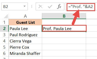
Here’s how you can use it to add text to the beginning of all cells in a range. Let us assume you have the following list of names and want to add the title “Prof.” before every name:

Below are the  steps to add  a text before a text string in Excel:

1. Click on the first cell of the column where you want the converted names to appear (B2).
2. Type equal sign (=), followed by the text “Prof. “, followed by an ampersand (&).
3. Select the cell containing the first name (A2).
4. Press the Return Key.
5. You will notice that the title “Prof.” is added before the first name in the list.
6. It’s now time to copy this formula to the rest of the cells in the column. Simply double click the fill handle (located at the bottom right of cell B2). Alternatively, you can drag down the fill handle to achieve the same effect.

That’s it, all your cells in column B should now contain the title “Prof.” preceding each name.

Using the ampersand Operator to Add Text to the End of all Cells

Now let us see how to add some text to the end of every name in the dataset. Let us say you want to add the text “(MD)” at the end of every name. In that case, here are the steps you need to follow:

1. Click on the first cell of the column where you want the converted names to appear (C2 in our case).
2. Type equal sign (=)
3. Select the cell containing the first name (B2 in our case).
4. Next, insert an ampersand (&), followed by the text “ (MD)”.
5. Press the Return Key.
6. You will notice that the text “(MD).” added after the first name in the list.
7. It’s now time to copy this formula to the rest of the cells in the column. Simply double click the fill handle (located at the bottom right of cell C2). Alternatively, you can drag down the fill handle to achieve the same effect.

All your cells in column C should now contain the text “(MD”) at the end of each name.

Method 2: Using the CONCATENATE Function

CONCATENATE is an Excel function that you can use to add text at the beginning and end of the text string.

Let’s see how to use CONCATENATE to do this.

Using CONCATENATE to Add Text to the Beginning of all Cells

The CONCATENATE() function provides the same functionality as the ampersand (&) operator. The only difference is in the way both are used.

The general syntax for the CONCATENATE function is:

=CONCATENATE(text1, [text2], …)

Where text1, text2, etc. are substrings that you want to combine together.

Let’s apply the CONCATENATE function to the same dataset as above:

1. Click on the first cell of the column where you want the converted names to appear (B2).
2. Type equal sign (=).
3. Enter the function CONCATENATE, followed by an opening bracket (.
4. Type the title “Prof. ” in double-quotes, followed by a comma (,).
5. Select the cell containing the first name (A2)
6. Place a closing bracket. In our example, your formula should now be: =CONCATENATE(“Prof. “,A2).
7. Press the Return Key.
8. You will notice that the title “Prof.” is added before the first name on the list.
9. It’s now time to copy this formula to the rest of the cells in the column. Simply double click the fill handle (located at the bottom right of cell B2). Alternatively, you can drag down the fill handle to achieve the same effect.

That’s it, all your cells in column B should now contain the title “Prof.” preceding each name.

Using CONCATENATE to Add Text to the End of all Cells

Now let us see how to add some text to the end of every name in the dataset. Let us say you want to add the text “(MD)” at the end of every name. In that case, here are the steps you need to follow:

1. Click on the first cell of the column where you want the converted names to appear (C2 in our example).
2. Type equal sign (=).
3. Enter the function CONCATENATE, followed by an opening bracket (.
4. Select the cell containing the first name (B2 in our example).
5. Next, insert a comma, followed by the text “ (MD)”.
6. Place a closing bracket. In our example, your formula should now be: =CONCATENATE(B2,” (MD)”).
7. Press the Return Key.
8. You will notice that the text “(MD).” added after the first name in the list.
9. It’s now time to copy this formula to the rest of the cells in the column. Simply double click the fill handle (located at the bottom right of cell C2).

All your cells in column C should now contain the text “(MD”) at the end of each name.

Notice that since you’re using a formula, your column C depends on columns A and B. So if you make any changes to the original values in column A, they get reflected in column C.

If you decide to only retain the converted names and delete columns A and B, you will get an error, as shown below:

To make sure that this does not happen, it’s best to first convert the formula results to permanent values copying them and pasting them as values in the same column (Right-click and select Paste Options->Values from the Popup menu).

Now you can go ahead and delete columns A and B if you need to.

Also read: How to Remove First Character in Excel?

Method 3: Using the Flash Fill Feature

Flash fill is a relatively new feature that looks at the pattern of what you are trying to achieve and then does it for all the cells in a column.

You can also use Flash fill to so text manipulation as we will see in the following examples.

Using Flash Fill to Add Text to the Beginning of all Cells

The Excel flash fill feature is like a magical button. It is available if you’re on any Excel version from 2013 onwards.

The feature takes advantage of Excel’s pattern recognition capabilities. It basically recognizes a pattern in your data and automatically fills in the other cells of the column with the same pattern for you.

Here’s how you can use Flash Fill to add text to the beginning of all cells in a column:

1. Click on the first cell of the column where you want the converted names to appear (B2).
2. Manually type in the text Prof. , followed by the first name of your list.
3. Press the Return Key.
4. Click on cell B2 again.
5. Under the Data tab, click on the Flash Fill button (in the ‘Data Tools’ group). Alternatively, you can just press CTRL+E on your keyboard (Command+E if you’re on a Mac).

This will copy the same pattern to the rest of the cells in the column… in a flash!

Using Flash Fill to Add Text to the End of all Cells in a Column

If you want to add the text “ (MD)” to the end of the names, follow the same steps:

1. Click on the first cell of the column where you want the converted names to appear (C2).
2. Manually type in or copy the text from column B2 into C2.
3. Add the text “(MD)” after that.
4. Under the Data tab, click on the Flash Fill or press CTRL+E on your keyboard (Command+E if you’re on a Mac).

That’s all, you get every cell filled in with the same pattern!

We especially like this method because it is simple, quick, and easy. Moreover, since it’s formula-free, the results do not depend on the original columns.

So they remain unchanged even if you delete rows A and B!

Method 4: Using VBA Code

And of course, if you’re comfortable with VBA, you can also add text before or after a text string using it.

Using VBA to Add Text to the Beginning of all Cells in a Column

If coding with VBA does not intimidate you then this method can help get your work done quickly too.

Here’s the code we will be using to add the title “Prof. “ to the beginning of all cells in a range. You can select and copy it:

Sub add_text_to_beginning()
Dim rng As Range
Dim cell As Range
Set rng = Application.Selection
For Each cell In rng
cell.Offset(0, 1).Value = "Prof. " & cell.Value
Next cell
End Sub

Follow these steps to use the above code:

1. From the Developer Menu Ribbon, select Visual Basic.
2. Once your VBA window opens, Click Insert->Module. Now you can start coding. Type or copy-paste the above lines of code into the module window. Your code is now ready to run.
3. Select the range of cells containing the text you want to convert. Make sure the column next to it is blank because this is where the code will display the results.
4. Navigate to Developer->Macros-> add_text_to_beginning->Run.

You will now see the converted text next to your selected range of cells.

Note: You can change the text in line 6 from “Prof. ” to whatever text you need to add to the beginning of all cells.

Using VBA to Add Text to the End of all Cells in a Column

Now, what if you want to add text to the end of all the cells, instead of the beginning? This only involves making a tweak to line 6 of the above code. So if you want to add the text “ (MD)” to the end of all cells, change line 6 to:

cell.Offset(0, 1).Value = cell.Value & “ (MD)”

So your full code should now be:

Sub add_text_to_end()
Dim rng As Range
Dim cell As Range
Set rng = Application.Selection
For Each cell In rng
cell.Offset(0, 1).Value = cell.Value & " (MD)"
Next cell
End Sub

Here’s the final result:

You can now delete the first two columns if you need to. Do remember to keep a backup of your sheet, because the results of VBA code are usually irreversible.

Note: You can change the text in line 6 from “ (MD)” to whatever text you need to add to the end of all cells in the range.

In this tutorial, we showed you four ways in which you can add text to the beginning and/ or end of all cells in a range.

There are plenty of other methods that you can find online too, and all of them work just as well as the ones shown here.

You may feel free to choose whatever method suits you, your requirement, and your version of Excel. In the end, what matters is getting what you need to be done quickly and effectively.

Other Excel tutorials you may like:

• How to Remove Text after a Specific Character in Excel
• How to Reverse a Text String in Excel
• How to Count How Many Times a Word Appears in Excel
• How to Remove Commas in Excel (from Numbers or Text String)
• How to Remove a Specific Character from a String in Excel
• How to Change Uppercase to Lowercase in Excel
• How to Separate Address in Excel?
• How to Concatenate with Line Breaks in Excel?
• How to Separate Names in Excel

Formulas are the life and blood of Excel spreadsheets. And in most cases, you don’t need the formula in just one cell or a couple of cells.

In most cases, you would need to apply the formula to an entire column (or a large range of cells in a column).

And Excel gives you multiple different ways to do this with a few clicks (or a keyboard shortcut).

Let’s have a look at these methods.

By Double-Clicking on the AutoFill Handle

One of the easiest ways to apply a formula to an entire column is by using this simple mouse double-click trick.

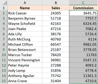
Suppose you have the dataset as shown below, where want to calculate the commission for each sales rep in Column C (where the commission would be 15% of the sale value in column B).

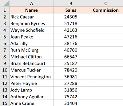
The formula for this would be:

=B2*15%

Below is the way to apply this formula to the entire column C:

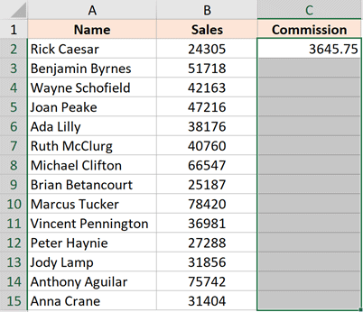
1. In cell A2, enter the formula: =B2*15%
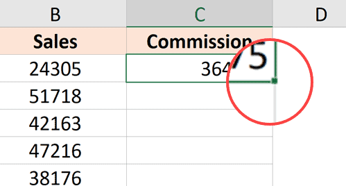
2. With the cell selected, you will see a small green square at the bottom-right part of the selection.
3. Place the cursor over the small green square. You will notice that the cursor changes to a plus sign (this is called the autofill handle)
4. Double click the left mouse key

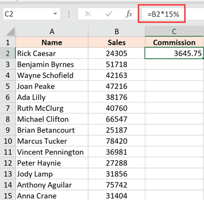
The above steps would automatically fill the entire column till the cell where you have the data in the adjacent column. In our example, the formula would be applied till cell C15

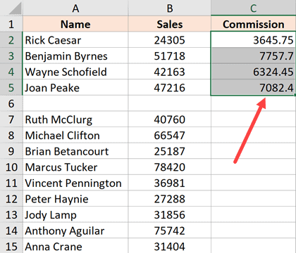
For this to work, there shouldn’t be data in the adjacent column and there should not be any blank cells in it. If, for example, there is a blank cell in column B (say cell B6), then this auto-fill double click would only apply the formula till cell C5

When you use the autofill handle to apply the formula to the entire column, it’s equivalent to copy-pasting the formula manually. This means that the cell reference in the formula would change accordingly.

For example, if it’s an absolute reference, it would remain as is while the formula is applied to the column, add if it’s a relative reference, then it would change as the formula is applied to the cells below.

By Dragging the AutoFill Handle

One issue with the above double click method is that it would stop as soon as it encountered a blank cell in the adjacent columns.

If you have a small data set, you can also manually drag the fill handle to apply the formula in the column.

Below are the steps to do this:

1. In cell A2, enter the formula: =B2*15%
2. With the cell selected, you will see a small green square at the bottom-right part of the selection
3. Place the cursor over the small green square. You will notice that the cursor changes to a plus sign
4. Hold the left mouse key and drag it to the cell where you want the formula to be applied
5. Leave the mouse key when done

Using the Fill Down Option (it’s in the ribbon)

Another way to apply a formula to the entire column is by using the fill down option in the ribbon.

For this method to work, you first need to select the cells in the column where you want to have the formula.

Below are the steps to use the fill down method:

1. In cell A2, enter the formula: =B2*15%
2. Select all the cells in which you want to apply the formula (including cell C2)
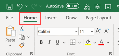
3. Click the Home tab
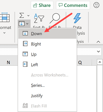
4. In the editing group, click on the Fill icon
5. Click on ‘Fill down’

The above steps would take the formula from cell C2 and fill it in all the selected cells

Adding the Fill Down in the Quick Access Toolbar

If you need to use the fill down option often, you can add that to the Quick Access Toolbar, so that you can use it with a single click (and it’s always visible on the screen).

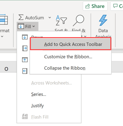
T0 add it to the Quick Access Toolbar (QAT), go to the ‘Fill Down’ option, right-click on it, and then click on ‘Add to the Quick Access Toolbar’

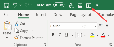
Now, you will see the ‘Fill Down’ icon appear in the QAT.

Using Keyboard Shortcut

If you prefer using the keyboard shortcuts, you can also use the below shortcut to achieve the fill down functionality:

CONTROL + D (hold the control key and then press the D key)

Below are the steps to use the keyboard shortcut to fill-down the formula:

1. In cell A2, enter the formula: =B2*15%
2. Select all the cells in which you want to apply the formula (including cell C2)
3. Hold the Control key and then press the D key

Using Array Formula

If you’re using Microsoft 365 and have access to dynamic arrays, you can also use the array formula method to apply a formula to the entire column.

Suppose you have a data set as shown below and you want to calculate the Commission in column C.

Below is the formula that you can use:

=B2:B15*15%

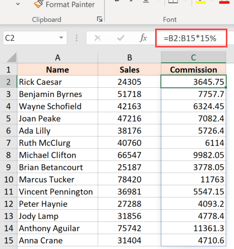
This is an Array formula that would return 14 values in the cell (one each for B2:B15). But since we have dynamic arrays, the result would not be restricted to the single-cell and would spill over to fill the entire column.

Note that you cannot use this formula in every scenario. In this case, because our formula uses the input value from an adjacent column and as the same length of the column in which we want the result (i.e., 14 cells), it works fine here.

But if this is not the case, this may not be the best way to copy a formula to the entire column

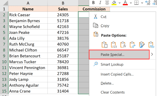
By Copy-Pasting the Cell

Another quick and well-known method of applying a formula to the entire column (or selected cells in the entire column) is to simply copy the cell that has the formula and paste it over those cells in the column where you need that formula.

Below are the steps to do this:

1. In cell A2, enter the formula: =B2*15%
2. Copy the cell (use the keyboard shortcut Control + C in Windows or Command + C in Mac)
3. Select all the cells where you want to apply the same formula (excluding cell C2)
4. Paste the copied cell (Control + V in Windows and Command + V in Mac)

One difference between this copy-paste method and all the methods convert below above this is that with this method you can choose to only paste the formula (and not paste any of the formattings).

For example, if cell C2 has a blue cell color in it, all the methods covered so far (except the array formula method) would not only copy and paste the formula to the entire column but also paste the formatting (such as the cell color, font size, bold/italics)

If you want to only apply the formula and not the formatting, use the steps below:

1. In cell A2, enter the formula: =B2*15%
2. Copy the cell (use the keyboard shortcut Control + C in Windows or Command + C in Mac)
3. Select all the cells where you want to apply the same formula
4. Right-click on the Selection
5. In the options that appear, click on ‘Paste Special’
6. In the ‘Paste Special’ dialog box, click on the Formulas option
7. Click OK

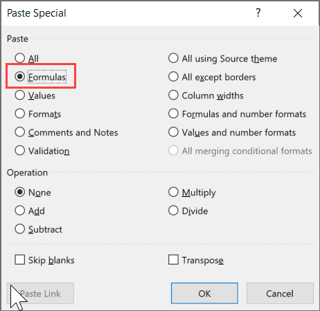
The above steps would make sure that only the formula is copied to the selected cells (and none of the formattings comes over with it).

So these are some of the quick and easy methods that you can use to apply a formula to the entire column in Excel.

I hope you found this tutorial useful!

Other Excel tutorials you may also like:

• 5 Ways to Insert New Columns in Excel (including Shortcut & VBA)
• How to Sum a Column in Excel
• How to Compare Two Columns in Excel (for matches & differences)
• Lookup and Return Values in an Entire Row/Column in Excel
• How to Copy and Paste Columns in Excel?
• Apply Conditional Formatting Based on Another Column in Excel
• How to Multiply a Column by a Number in Excel