
Excel Toolbar (Table of Contents)
- Toolbar in Excel
- How to Use the Toolbar in Excel?
The Toolbar is an area where you can add different commands or tools associated with excel. By default, it is located above the ribbon with different tools and visible in the Excel window’s upper right corner. To increase customer friendliness, toolbars have become customizable according to the frequent use of different tools. Instead of a set of tools, excel gives us the option to select and build a Quick Access Toolbar. This makes quick access to the tools that you want. So the toolbar is popularly known as Quick Access Toolbar.

It is a symbolical representation of built-in options available in Excel. By default, it contains the below commands.
- Save: To save the created workbook.
- Undo: To return or step back one level of an immediate action performed.
- Redo: Repeat the last action.
How to Use the Toolbar in Excel?
The Toolbar in Excel is a shortcut tool to avoid searching for the commands you often use in the worksheet. Using Toolbar in Excel is easy, and it helps us simplify access to the document’s commands. Let’s understand the working of the Toolbar in Excel by some examples given below.
Example #1
Adding Commands to the Toolbar in Excel
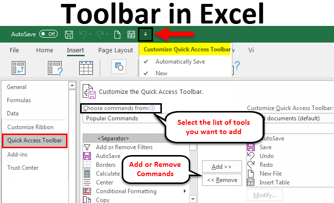
To get more tools, you have the option to customize the Quick Access Toolbar simply by adding the commands.
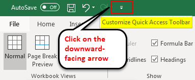
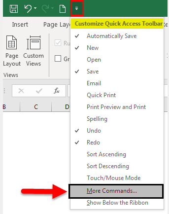
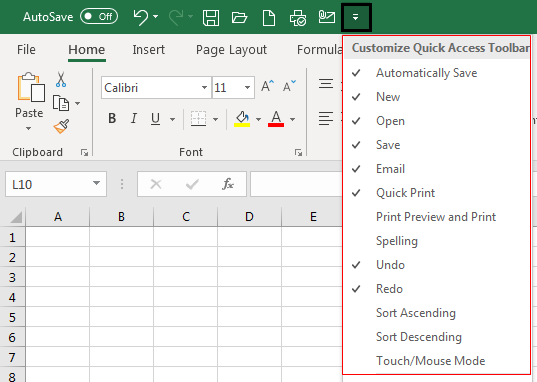
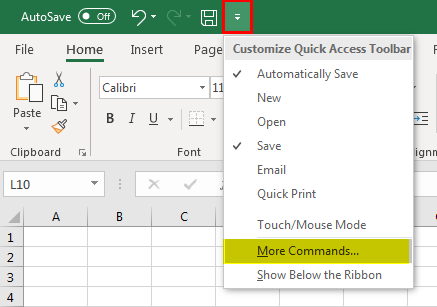
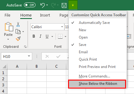
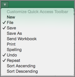
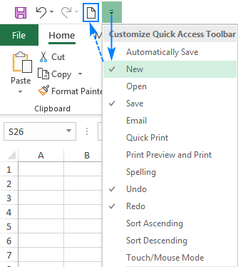
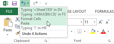
- Click on the downward-facing arrow at the end of the Toolbar in Excel. A pop up will be shown as Customize Quick Access Toolbar.
- From the dropdown, you will get a list of commonly used commands. Click any of the options that you want, and it will be added to the toolbar.
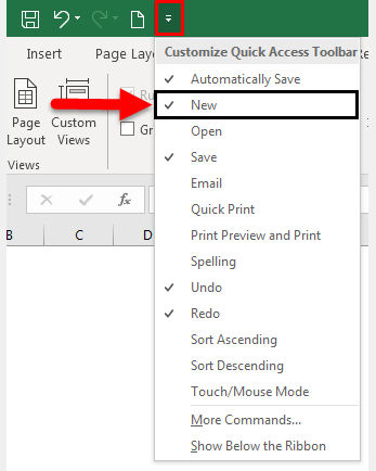
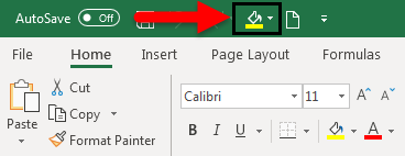
- A new command is selected, and this will be added to the toolbar highlighted as the command is added with already available tools.
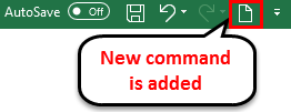
In a similar way, you can add the tools which you want to access quickly. So instead of clicking and finding the tools from the multiple hierarchies, you can access the option within a single click.
Example #2
Adding Commands to the Toolbar in Excel
There are options to add more tools Instead of the listed commands. You can add more commands to the quick Access Toolbar by selecting More Commands.
- Click on the downward-facing arrow at the end of the toolbar. Select the More Commands option.
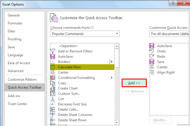
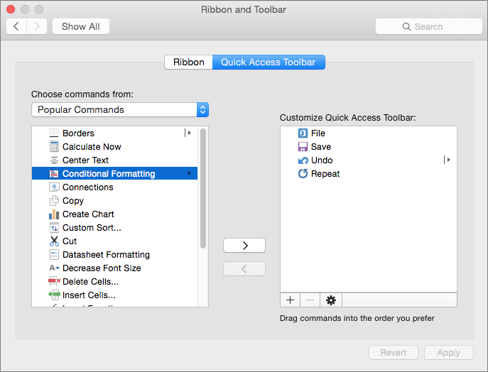
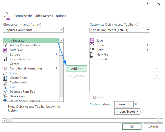
- You will get a new window which gives you all the options available with excel to add to your toolbar.
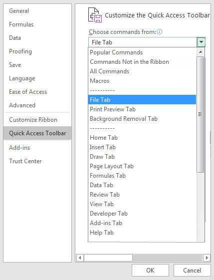
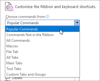
From the Choose commands from the drop-down, you can select which list of tools you want to add. Each list will lead to a different list of commands that you can add to the toolbar.
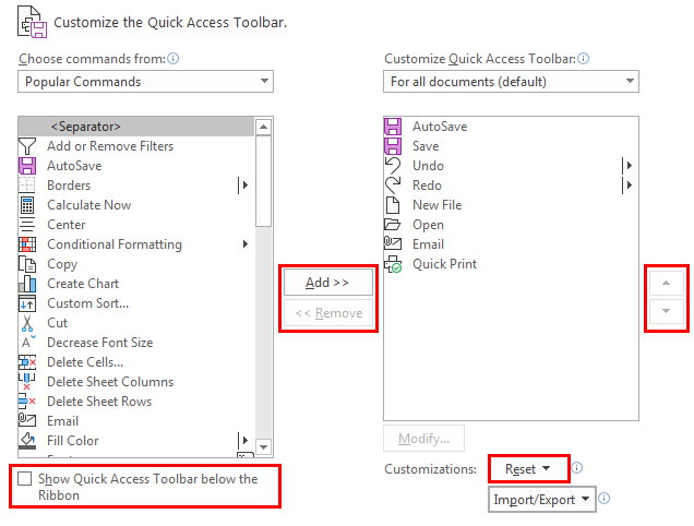
- Click on the Popular Commands, which shows the set of most commonly used commands. Select the Fill color which you want to add to the toolbar. You can see an add button right next to the list of commands; by pressing it and clicking on the OK button, you can add the selected tool to the Excel Toolbar.
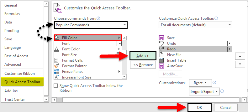
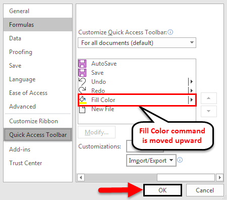
- Once you add the command, it will appear in the list next to the add button. This is the list of tools added to the Toolbar. The “Fill Color” command will be added to the Customize Quick Access Toolbar.
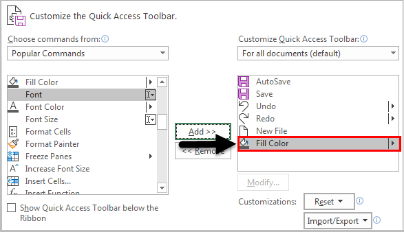
- You can see the “Fill Color” command added to the Quick Access Toolbar as below and the existing commands. Since this is the last item added to the Quick Access Toolbar, it will appear in the listed order.
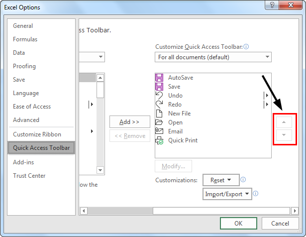
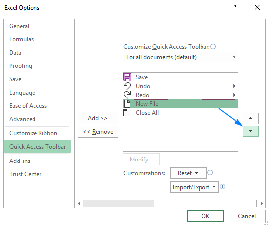
- To reorder the added items, you can use the up and down arrow highlighted on the right to the list of items.
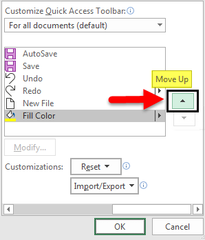
- Select the command which you want to reorder or change the position. By clicking the Upward arrow, the “Fill Color” command is moved upwards in the list shown as below.
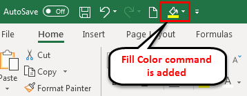
- By pressing the OK button, the selected format will be applied to the Quick Access Toolbar. The “Fill Color” Command is visible before the “New File” Tool.
You can see the visibility order of the listed tools is changed. According to the new list order, the “Fill Color” position has been changed to the second last from the end.
Example #3
Removing Command
The commands can be removed from the quick access toolbar if you are no longer using them or not using them frequently. The commands can be removed in a similar way to how you added the commands to the Quick Access Toolbar.
- Click on the downward-facing arrow at the end of the toolbar. Select the More Commands option.
- You will get a new window which will show the already added commands on the right side. This is the list of commands which are already in the quick access toolbar.
- Select the command which you want to remove from the quick access toolbar. In the center, below the add button, a Remove button will be enabled. Press the OK button to make the applied changes.
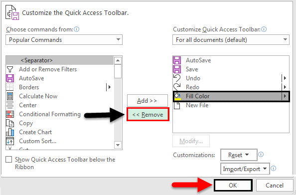
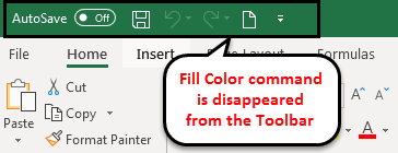
- The Fill Color command is removed, and it will be disappeared from the Quick Access Toolbar, as shown below.
Example #4
Moving the Position
According to your convenience, you can change the position of the toolbar. You can change the position from top to below the ribbon or vice versa.
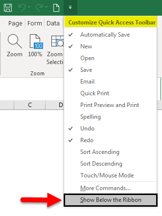
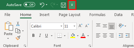
- Select the downward-facing arrow at the end of the toolbar, then select the Show Below the Ribbon option from the list.
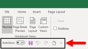
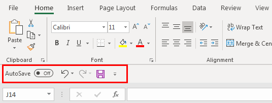
- Now the Toolbar is moved below to the ribbon.
Example #5
Adding Ribbon Commands
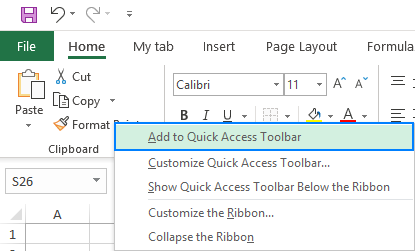
- Right-click on the tool within the ribbon which you want to add to the Toolbar in Excel. You will get the option to Add to Quick Access Toolbar. Here we right-clicked on the Table tool to add from the insert command.
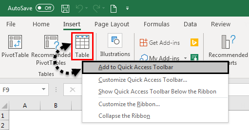
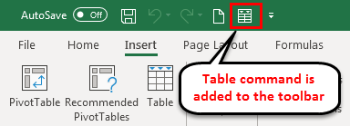
- The command will be added to the Quick Access Toolbar as below.
Things to Remember
- Similar to the name Quick Access Toolbar, this is a customizable toolbar to access the tools easily.
- It is possible to add any of the available commands in excel to the Excel Toolbar.
- The visibility of the toolbar can be set above or below the ribbon.
- Just through a right-click, you will get the option to add most of the command to the Toolbar in Excel.
Recommended Articles
This has been a guide to Toolbar in excel. Here we have discussed How to Use and Customize the Toolbar in Excel, along with practical examples. You can also go through our other suggested articles –
- Excel Shortcut For Merge Cells
- Insert New Worksheet In Excel
- Table Styles in Excel
- Add Rows in Excel Shortcut
Toolbar or we can say it is a Quick Access Toolbar available in Excel on the left top side of the Excel window. By default, it has only a few options such as “Save,” “Redo,” and “Undo,” but we can customize the toolbar as per our choice and insert any option or button in the toolbar which will help us to reach the commands to use more quickly than before.
Table of contents
- Excel Toolbar
- How to Use the toolbar in Excel?
- Examples to Understand Quick Access Excel Toolbar
- 1 – Adding Features to the Toolbar
- Method 1
- Method 2
- Method 3
- #2 – Deleting Features from the Toolbar
- #3 – Moving the Toolbar on the Ribbon
- #4 – Modifying the Sequence of Commands and Resetting to Default Settings.
- #5 – Customize Excel Toolbar
- #6 – Exporting and Importing of Quick Access Toolbar
- 1 – Adding Features to the Toolbar
- Things to Remember
- Recommended Articles
Excel toolbar (also called Quick Access ToolbarQuick Access Toolbar (QAT) is a toolbar in Excel that may be customized and is located on the upper left-hand side of the window. It enables users to save important shortcuts and easily access them when needed.read more) is presented to access various commands to perform the operations. In addition, it is presented with an option to add or delete commands to it to access them quickly.
- Quick Access Toolbar is universal, and access is possible on any tab like “Home,” “Insert,” “Review,” “References,” etc. It is independent of the tab that we are working on simultaneously.
- It contains the various options used frequently to enhance the speed of working in Excel sheets.
- Along with the Quick Access Toolbar, another toolbar such as the “Formula Bar,” “Headings,” and Gridlines in excelGridlines are little lines made of dots to divide cells from each other in a worksheet. The gridlines have slight faint invisibility; you can find it in the page layout tab. This option has a checkbox; for activating the gridlines, you can tick on it and untick if you wish to deactivate gridlines.read more under the “Show” or “Hide” group of the “View” tab simply selecting and deselecting the checkmark shows or hides this toolbar.
- “Format” toolbar, “Drawing” toolbar, “Chart” toolbar, and “Standard” toolbar presented in the earlier version of Excel 2003 are modified into the “Home” tab and “Insert” tab in the later versions of Excel 2007 and more.
- The “Customize Quick Access Toolbar” option is available to access the full toolbars list.
How to Use the toolbar in Excel?
- The toolbar in Excel is used for various purposes. However, few major activities are performed on the Quick Access Toolbar on different versions of Excel.
- In the 2007 version, only three activities shift the toolbar’s location, including adding extra features or frequently used commands. In addition, deleting an element from the toolbar is possible whenever we do not want to.
- In higher versions than in 2007, the Quick Access Toolbar is used in many ways, along with adding and removing commands. These include adding commands not presented on the toolbar, modifying commands order, moving the toolbar below or above the ribbon, grouping two or more commands, exporting and importing the toolbar, customizing utilizing the “Options” command, and resetting the default settings.
- Frequent commands like “Save,” “Open,” “Redo,” “New,” “Undo,” “Email,” “Quick Print,” and print preview in excelPrint preview in Excel is a tool used to represent the print output of the current page in the excel to see if any adjustments need to be made in the final production. Print preview only displays the document on the screen, and it does not print.read more are easily added to the toolbar.
- We can select the commands not listed in the toolbar from the three categories, including “Popular Commands,” “All Commands,” and “Commands Not Listed” on the ribbon.
Examples to Understand Quick Access Excel Toolbar
Below are examples of the Excel toolbar.
1 – Adding Features to the Toolbar
Adding features or commands to the Quick Access Toolbar is essential. It is done in three ways:
- Adding commands located on the ribbon
- Adding features through the “More Commands” option
- Adding the elements presented on the different tabs directly to the toolbar
Method 1
We can add “New,” “Open,” “Save,” “Email,” “Quick Print,” and redo in excelIn Excel, we have an option named “Undo” that we may use by pressing Ctrl + Z. When we undo an action but subsequently realize it was not a mistake, we can cancel the undo action and return to the original point, using «Redo.»read more features to the toolbar. For that, select the “Customize Quick Access Toolbar” button and click on the command you want to add to the toolbar.
In the above figure, we can see the tick-marked option present in the toolbar.
Method 2
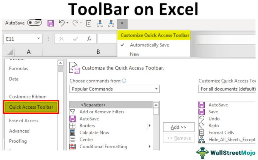
In this, a user must select the “Customize Quick Access Toolbar” in Excel and select the “More Commands” option to add the commands.
As shown in the below figure of the customize window, the user must select the commands and click on the “Add” option to add the feature to the toolbar. Added features are displayed on the excel ribbonThe ribbon is an element of the UI (User Interface) which is seen as a strip that consists of buttons or tabs; it is available at the top of the excel sheet. This option was first introduced in the Microsoft Excel 2007.read more for accessing easily.
Method 3
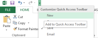
The user has to right-click on the feature presented on the ribbon and choose “Add to Quick Access Toolbar.”

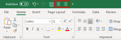
As shown in the figure, center and right alignment commands are added to the toolbar utilizing this option.
#2 – Deleting Features from the Toolbar
To remove commands,
- Go to “More Commands.”

- Select the command that wants to be removed under the “Customize Quick Access Toolbar” option.

- Then, click on the “Remove” button to remove the selected command.

We can also do it by selecting “Excel Options” by clicking on the Microsoft office button on the top left corner of the window and then going to the “Customize” tab.
#3 – Moving the Toolbar on the Ribbon
If a user wants to shift the toolbar to another location, it is done in a few steps. First, the toolbar can be presented below or above the ribbon.
To present the toolbar below the ribbon:
- Click on the “Customize Quick Access Toolbar” button.
- Select the options shown below the ribbon.
#4 – Modifying the Sequence of Commands and Resetting to Default Settings.
The up and down buttons on the “Customize Quick Access Toolbar” present the option in the order per user. Users can discard the changes by clicking on the “Reset” option to get the default settings.
#5 – Customize Excel Toolbar
Customizing the Excel toolbar is done to add, remove, reset, change the toolbar’s location, modify, and alter the order of the features at a time.
All operations are performed quickly on the toolbar using the customization option.
#6 – Exporting and Importing of Quick Access Toolbar
Exporting and importing features are presented in the latest versions of Excel to have the same settings for files used by another computer. To do this,
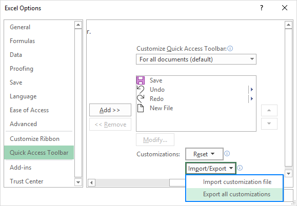
- Go to “File” and select “Options.”
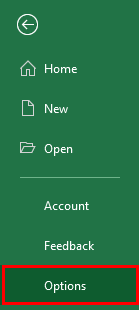
- Then go to a “Quick Access Toolbar.”
- Choose the “Import/Export” option to export customized settings.
Use the same steps to import customization.
Things to Remember
- The Quick Access Toolbar does not have a feature of displaying multiple lines.
- It is hard to enhance the size of the buttons to correspond to the commands. It is done only by changing the resolution of the screen.
- Another way to add commands to the toolbar is that right-clicking on the ribbon facilitates the option.
- Contents of several commands such as styles, indent, and spacing are not added to the toolbar but are represented in the form of buttons.
- Keyboard shortcutsAn Excel shortcut is a technique of performing a manual task in a quicker way.read more are also applied to the commands presented on the toolbar. For example, pressing the “ALT” key displays the shortcut numbers to utilize the commands more effectively by reducing the time.
Recommended Articles
This article is a guide to Toolbar on Excel. Here, we discuss how to add, delete, and modify features on the toolbar and how to customize the Excel toolbar. You can learn more about Excel from the following articles: –
- What does Rows Function do in Excel?
- Compare Excel Rows vs. Columns
- Analysis ToolPak in Excel
- Excel Translate
What you can customize: You can personalize your ribbon to arrange tabs and commands in the order you want them, hide or unhide your ribbon, and hide those commands you use less often. Also, you can export or import a customized ribbon.
What you can’t customize: You can’t reduce the size of your ribbon, or the size of the text or the icons on the ribbon. The only way to do this is to change your display resolution, which would change the size of everything on your page.
When you customize your ribbon: Your customizations apply only to the Office program you’re working in at the time. For example, if you personalize your ribbon in PowerPoint, those same changes won’t be visible in Excel. If you want similar customizations in your other Office apps, you’ll have to open each of those apps to make the same changes. Although you can’t share customizations between apps, you can export your customizations to share with others or use on other devices.
Tip: You can’t change the color of the ribbon, or its icons, but you can change the color scheme that Office uses throughout. For more information see Change the Office theme.
You can toggle between having the ribbon expanded or collapsed in multiple ways.
If the ribbon is collapsed, expand it by doing do one of the following:
-
Double-click any of the ribbon tabs.
-
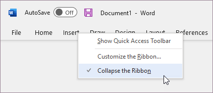
Right-click any of the ribbon tabs, and then select Collapse the ribbon.

-
Press CTRL+F1.
If the ribbon is expanded, collapse it by doing do one of the following:
-
Double-click any of the ribbon tabs.
-
Right-click any of the ribbon tabs, and then select Collapse the ribbon.
-
Right-click Ribbon display options in the lower right of the ribbon, and then select Collapse the ribbon.
-
Press CTRL+F1.
If the ribbon isn’t visible at all
If the ribbon isn’t visible at all (no tabs are showing), then you probably have the state set to Full-screen mode. Select More at the top right of the screen. This will temporarily restore the ribbon.
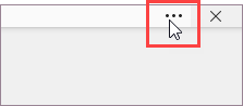
When you return to the document, the ribbon will be hidden again. To keep the ribbon displayed, select a different state from the Ribbon Display Options menu.
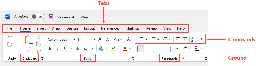
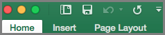
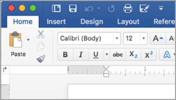
The tabs on your ribbon are Home, Insert, Design, etc. For example, the picture below shows the tabs in Word.
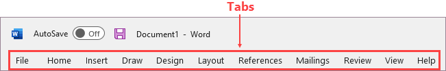
You can add custom tabs or rename and change the order of the default tabs that are built in to Office. Custom tabs in the Customize the Ribbon list have (Custom) after the name, but the word (Custom) does not appear in the ribbon.
Open the «Customize the Ribbon» window
To work with your ribbon, you need to get to the Customize the Ribbon window. Here’s how you do that.
-
Open the app you want to customize your ribbon in, such as PowerPoint or Excel.
-
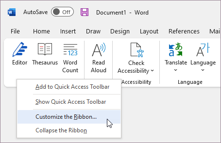
Place your mouse in any empty space in the ribbon and then right-click.
-
Click Customize the Ribbon.
Now you’re ready to do the steps below to customize your ribbon.
Change the order of default or custom tabs
You can change the order of Home, Insert, Draw, Design, and other tabs. You cannot change the placement of the File tab.
-
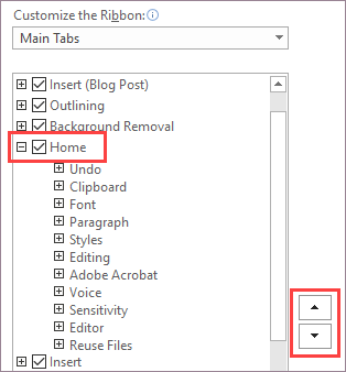
In the Customize the Ribbon window under the Customize the Ribbon list, click the tab that you want to move.
-
Click the Move Up or Move Down arrow until you have the order you want.
-
To see and save your changes, click OK.
Add a custom tab
When you click New Tab, you add a custom tab and custom group. You can only add commands to custom groups.
-
In the Customize the Ribbon window under the Customize the Ribbon list, click New Tab.
-
To see and save your changes, click OK.
Rename a default or custom tab
-
In the Customize the Ribbon window under the Customize the Ribbon list, click the tab that you want to rename.
-
Click Rename, and then type a new name.
-
To see and save your changes, click OK.
Hide a default or custom tab
You can hide both custom and default tabs. But you can only remove custom tabs. You cannot hide the File tab.
-
In the Customize the Ribbon window under the Customize the Ribbon list, clear the check box next to the default tab or custom tab that you want to hide.
-
To see and save your changes, click OK.
Remove a custom tab
You can hide both custom and default tabs, but you can only remove custom tabs. The custom tabs and groups have (Custom) after the name, but the word (Custom) does not appear in the ribbon.
-
In the Customize the Ribbon window under the Customize the Ribbon list, click the tab that you want to remove.
-
Click Remove.
-
To see and save your changes, click OK.
You can add custom groups or rename and change the order of the default groups that are built in to Office. Custom groups in the Customize the Ribbon list have (Custom) after the name, but the word (Custom) does not appear in the ribbon.
Change the order of the default and custom groups
-
In the Customize the Ribbon window under the Customize the Ribbon list, click the group that you want to move.
-
Click the Move Up or Move Down arrow until you have the order you want.
-
To see and save your changes, click OK.
Add a custom group to a tab
You can add a custom group to either a custom tab or a default tab.
-
In the Customize the Ribbon window, under the Customize the Ribbon list, click the tab that you want to add a group to.
-
Click New Group.
-
To rename the New Group (Custom) group, right-click the group, click Rename, and then type a new name.
Note: You can also add an icon to represent the custom group by clicking the custom group, then Rename. When the Symbol dialog opens, choose an icon to represent the group.
-
To hide the labels for the commands that you add to this custom group, right-click the group, and then click Hide Command Labels. Repeat to un-hide them.
-
To see and save your changes, click OK.
Rename a default or custom group
-
In the Customize the Ribbon window under the Customize the Ribbon list, click the tab or group that you want to rename.
-
Click Rename, and then type a new name.
-
To see and save your changes, click OK.
Remove a default or custom group
-
In the Customize the Ribbon window under the Customize the Ribbon list, click the group that you want to remove.
-
Click Remove.
-
To see and save your changes, click OK.
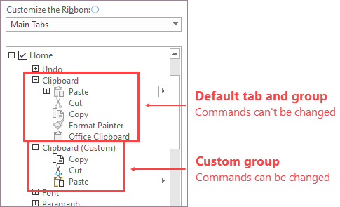
Replace a default group with a custom group
You can’t remove a command from a group built in to Microsoft Office. However, you can make a custom group with the commands that you want to replace the default group.
-
In the Customize the Ribbon window under the Customize the Ribbon list, click the default tab where you want to add the custom group.
-
Click New Group.
-
Right-click the new group, and then click Rename.
-
Type a name for the new group and select an icon to represent the new group when the ribbon is resized.
-
In the Choose Commands from list, click Main Tabs.
-
Click the plus sign (+) next to the default tab that contains the group that you want to customize.
-
Click the plus sign (+) next to the default group that you want to customize.
-
Click the command that you want to add to the custom group, and then click Add.
-
Right-click the default group, and click Remove.
To add commands to a group, you must first add a custom group to a default tab or to a new custom tab. Only commands added to custom groups can be renamed.
Default commands appear in gray text. You can’t rename them, change their icons, or change their order.
Change the order of the commands in custom groups
-
In the Customize the Ribbon window under the Customize the Ribbon list, click the command that you want to move.
-
Click the Move Up or Move Down arrow until you have the order you want.
-
To see and save your changes, click OK.
Add commands to a custom group
-
In the Customize the Ribbon window under the Customize the Ribbon list, click the custom group that you want to add a command to.
-
In the Choose commands from list, click the list you want to add commands from, for example, Popular Commands or All Commands.
-
Click a command in the list that you choose.
-
Click Add.
-
To see and save your changes, click OK.
Remove a command from a custom group
You can only remove commands from a custom group.
-
In the Customize the Ribbon window, under the Customize the Ribbon list, click the command that you want to remove.
-
Click Remove.
-
To see and save your changes, click OK.
Rename a command that you added to a custom group
-
In the Customize the Ribbon window under the Customize the Ribbon list, click the command that you want to rename.
-
Click Rename, and then type a new name.
-
To see and save your changes, click OK.
You can reset all tabs to their original state, or you can reset select tabs to their original state . When you reset all tabs on the ribbon, you also reset the Quick Access Toolbar to show only the default commands.
Follow these steps to reset the ribbon:
-
In the Customize the Ribbon window, click Reset.
-
Click Reset all customizations.
Reset only the selected tab to the default setting
You can only reset default tabs to their default settings.
-
In the Customize the Ribbon window, select the default tab that you want to reset to the default settings.
-
Click Reset, and then click Reset only selected Ribbon tab.
You can share your ribbon and Quick Access Toolbar customizations into a file that can be imported and used by a coworker or on another computer.
Step 1: Export your customized ribbon:
-
In the Customize the Ribbon window, click Import/Export.
-
Click Export all customizations.
Step 2: Import the customized ribbon and Quick Access Toolbar on your other computer
Important: When you import a ribbon customization file, you lose all prior ribbon and Quick Access Toolbar customizations. If you think that you might want to revert to the customization you currently have, you should export them before importing any new customizations.
-
In the Customize the Ribbon window, click Import/Export.
-
Click Import customization file.
Related Topics
Customize the Quick Access Toolbar
You can personalize the Ribbon and toolbars in Office just the way you like them, showing frequently used commands and hiding the ones you rarely use. You can change default tabs, or create custom tabs and custom groups to contain your frequently used commands.
Note: You cannot rename the default commands, change the icons associated with these default commands, or change the order of these commands.
-
To customize the Ribbon, open or create an Excel, Word, or PowerPoint document.
-
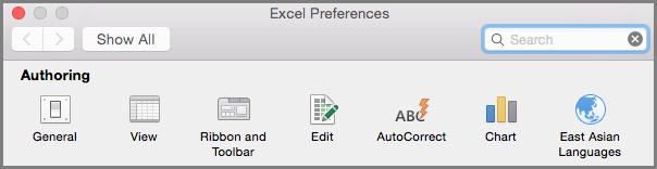
Go to the app Preferences and select Ribbon and Toolbar.
-
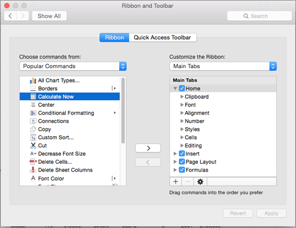
On the Ribbon tab window, select the commands you want to add or remove from your Ribbon and select the add or remove arrows.
Note: To remove the default tabs or commands like the Home or Insert tab from the Ribbon, uncheck the relevant checkbox in the Customize the Ribbon box.
Here’s what you can customize on the Ribbon:
-
Rename the tabs: To rename, select a tab, like Home, Insert, Design in the Customize the Ribbon box, select
> Rename. -
Add new tab or new group: To add new tab or new group, select
below the Customize the Ribbon box, and select New tab or New group. -
Remove tabs: You can remove custom tabs only from the Ribbon. To remove, select your tab in the Customize the Ribbon box and select
.
 > Rename.
 below the Customize the Ribbon box, and select New tab or New group.
 .
.Customize the Quick Access Toolbar
If you just want a few commands on your fingertips, you want to use the Quick Access Toolbar. Those are the icons that are above the Ribbon and they are always on no matter what tab you are on in the Ribbon.
-
To customize the Quick Access Toolbar, open or create an Excel, Word, or PowerPoint document.
-
Go to the app Preferences and select Quick Access Toolbar.
-
On the Quick Access Toolbar tab window, select the commands and select the arrows to add or remove from the Customize Quick Access Toolbar box.
Note: If you don’t see the commands to add to the Quick Access Toolbar, it is because we don’t support it at this time.
Once you select a command, it will appear at the end of the Quick Access toolbar.
Here are the default commands on the Quick Access Toolbar:
If you want just want to add one of these commands, just select the command name to add or remove it from the toolbar. Items that appear in the Quick Access Toolbar will have a checkmark
next to them.
 next to them.
Minimize or Expand the ribbon
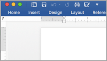
You can minimize the ribbon so that only the tabs appear.
|
Expanded ribbon |
Collapsed ribbon |
Minimize the ribbon while you are working
-
On the right side of the ribbon, select
.
 .
.Expand the ribbon while you are working
-
On the right side of the ribbon, select
.
 .
.Minimize the ribbon when a file opens
By default, the ribbon is expanded every time that you open a file, but you can change that setting so that the ribbon is always minimized.
-
On the View menu, clear the Ribbon check mark.
-
To once again display the ribbon when you open a file, on the View menu, select Ribbon or simply expand the ribbon by selecting
.
Содержание
- Toolbar on Excel
- Excel Toolbar
- How to Use the toolbar in Excel?
- Examples to Understand Quick Access Excel Toolbar
- 1 – Adding Features to the Toolbar
- #2 – Deleting Features from the Toolbar
- #3 – Moving the Toolbar on the Ribbon
- #4 – Modifying the Sequence of Commands and Resetting to Default Settings.
- #5 – Customize Excel Toolbar
- #6 – Exporting and Importing of Quick Access Toolbar
- Things to Remember
- Recommended Articles
- Quick Access Toolbar in Excel: how to customize, move, reset and share
- What is Quick Access Toolbar?
- Where is Quick Access Toolbar in Excel?
- How to customize Quick Access Toolbar in Excel
- Quick Access Toolbar: what can and what cannot be changed
- What can be customized
- What cannot be customized
- 3 ways to get to the Customize Quick Access Toolbar window
- How to add a command button to Quick Access Toolbar
- Enable a command from the predefined list
- Add a ribbon button to Quick Access Toolbar
- Add a command that isn’t on the ribbon to Quick Access Toolbar
- How to remove a command from Quick Access Toolbar
- Rearrange commands on Quick Access Toolbar
- Group commands on Quick Access Toolbar
- Add macros to Quick Access Toolbar in Excel
- Customize Quick Access Toolbar for the current workbook only
- How to move Quick Access Toolbar below or above the ribbon
- Reset Quick Access Toolbar to the default settings
- Export and import a custom Quick Access Toolbar


Toolbar or we can say it is a Quick Access Toolbar available in Excel on the left top side of the Excel window. By default, it has only a few options such as “Save,” “Redo,” and “Undo,” but we can customize the toolbar as per our choice and insert any option or button in the toolbar which will help us to reach the commands to use more quickly than before.
Table of contents
Excel toolbar (also called Quick Access Toolbar Quick Access Toolbar Quick Access Toolbar (QAT) is a toolbar in Excel that may be customized and is located on the upper left-hand side of the window. It enables users to save important shortcuts and easily access them when needed. read more ) is presented to access various commands to perform the operations. In addition, it is presented with an option to add or delete commands to it to access them quickly.
- Quick Access Toolbar is universal, and access is possible on any tab like “Home,” “Insert,” “Review,” “References,” etc. It is independent of the tab that we are working on simultaneously.
- It contains the various options used frequently to enhance the speed of working in Excel sheets.
- Along with the Quick Access Toolbar, another toolbar such as the “Formula Bar,” “Headings,” and Gridlines in excelGridlines In ExcelGridlines are little lines made of dots to divide cells from each other in a worksheet. The gridlines have slight faint invisibility; you can find it in the page layout tab. This option has a checkbox; for activating the gridlines, you can tick on it and untick if you wish to deactivate gridlines.read more under the “Show” or “Hide” group of the “View” tab simply selecting and deselecting the checkmark shows or hides this toolbar.
- “Format” toolbar, “Drawing” toolbar, “Chart” toolbar, and “Standard” toolbar presented in the earlier version of Excel 2003 are modified into the “Home” tab and “Insert” tab in the later versions of Excel 2007 and more.
- The “Customize Quick Access Toolbar” option is available to access the full toolbars list.
You are free to use this image on your website, templates, etc., Please provide us with an attribution link How to Provide Attribution? Article Link to be Hyperlinked
For eg:
Source: Toolbar on Excel (wallstreetmojo.com)
How to Use the toolbar in Excel?
- The toolbar in Excel is used for various purposes. However, few major activities are performed on the Quick Access Toolbar on different versions of Excel.
- In the 2007 version, only three activities shift the toolbar’s location, including adding extra features or frequently used commands. In addition, deleting an element from the toolbar is possible whenever we do not want to.
- In higher versions than in 2007, the Quick Access Toolbar is used in many ways, along with adding and removing commands. These include adding commands not presented on the toolbar, modifying commands order, moving the toolbar below or above the ribbon, grouping two or more commands, exporting and importing the toolbar, customizing utilizing the “Options” command, and resetting the default settings.
- Frequent commands like “Save,” “Open,” “Redo,” “New,” “Undo,” “Email,” “Quick Print,” and print preview in excelPrint Preview In ExcelPrint preview in Excel is a tool used to represent the print output of the current page in the excel to see if any adjustments need to be made in the final production. Print preview only displays the document on the screen, and it does not print.read more are easily added to the toolbar.
- We can select the commands not listed in the toolbar from the three categories, including “Popular Commands,” “All Commands,” and “Commands Not Listed” on the ribbon.
Examples to Understand Quick Access Excel Toolbar
Below are examples of the Excel toolbar.
1 – Adding Features to the Toolbar
Adding features or commands to the Quick Access Toolbar is essential. It is done in three ways:
- Adding commands located on the ribbon
- Adding features through the “More Commands” option
- Adding the elements presented on the different tabs directly to the toolbar
Method 1
In the above figure, we can see the tick-marked option present in the toolbar.
Method 2
In this, a user must select the “Customize Quick Access Toolbar” in Excel and select the “More Commands” option to add the commands.
As shown in the below figure of the customize window, the user must select the commands and click on the “Add” option to add the feature to the toolbar. Added features are displayed on the excel ribbon Excel Ribbon The ribbon is an element of the UI (User Interface) which is seen as a strip that consists of buttons or tabs; it is available at the top of the excel sheet. This option was first introduced in the Microsoft Excel 2007. read more for accessing easily.
Method 3
The user has to right-click on the feature presented on the ribbon and choose “Add to Quick Access Toolbar.”
As shown in the figure, center and right alignment commands are added to the toolbar utilizing this option.
#2 – Deleting Features from the Toolbar
To remove commands,
Select the command that wants to be removed under the “Customize Quick Access Toolbar” option.
Then, click on the “Remove” button to remove the selected command.

We can also do it by selecting “Excel Options” by clicking on the Microsoft office button on the top left corner of the window and then going to the “Customize” tab.
#3 – Moving the Toolbar on the Ribbon
If a user wants to shift the toolbar to another location, it is done in a few steps. First, the toolbar can be presented below or above the ribbon.
To present the toolbar below the ribbon:
- Click on the “Customize Quick Access Toolbar” button.
- Select the options shown below the ribbon.
#4 – Modifying the Sequence of Commands and Resetting to Default Settings.
The up and down buttons on the “Customize Quick Access Toolbar” present the option in the order per user. Users can discard the changes by clicking on the “Reset” option to get the default settings.
#5 – Customize Excel Toolbar
Customizing the Excel toolbar is done to add, remove, reset, change the toolbar’s location, modify, and alter the order of the features at a time.
All operations are performed quickly on the toolbar using the customization option.
#6 – Exporting and Importing of Quick Access Toolbar
Exporting and importing features are presented in the latest versions of Excel to have the same settings for files used by another computer. To do this,
- Go to “File” and select “Options.”
- Then go to a “Quick Access Toolbar.”
- Choose the “Import/Export” option to export customized settings.
Use the same steps to import customization.
Things to Remember
- The Quick Access Toolbar does not have a feature of displaying multiple lines.
- It is hard to enhance the size of the buttons to correspond to the commands. It is done only by changing the resolution of the screen.
- Another way to add commands to the toolbar is that right-clicking on the ribbon facilitates the option.
- Contents of several commands such as styles, indent, and spacing are not added to the toolbar but are represented in the form of buttons.
- Keyboard shortcutsKeyboard ShortcutsAn Excel shortcut is a technique of performing a manual task in a quicker way.read more are also applied to the commands presented on the toolbar. For example, pressing the “ALT” key displays the shortcut numbers to utilize the commands more effectively by reducing the time.
Recommended Articles
This article is a guide to Toolbar on Excel. Here, we discuss how to add, delete, and modify features on the toolbar and how to customize the Excel toolbar. You can learn more about Excel from the following articles: –
Источник
 by Svetlana Cheusheva, updated on March 16, 2023
In this tutorial, we will have an in-depth look at how to use and customize Quick Access Toolbar in Excel 2010, Excel 2013, Excel 2016, Excel 2019, Excel 2021 and Excel 365.
Getting to the commands you use most often should be easy. And it is exactly what the Quick Access Toolbar is designed for. Add your favorite commands to the QAT so they are only a click away no matter what ribbon tab you currently have open.
The Quick Access Toolbar (QAT) is a small customizable toolbar at the top of the Office application window that contains a set of frequently used commands. These commands can be accessed from almost any part of the application, independent of the ribbon tab that is currently opened.
The Quick Access Toolbar has a drop-down menu containing a predefined set of the default commands, which may be displayed or hidden. Additionally, it includes an option to add your own commands.
There is no limit to a maximum number of commands on the QAT, although not all the commands may be visible depending on the size of your screen.
By default, the Quick Access Toolbar is located in the upper left corner of the Excel window, above the ribbon. If you want QAT to be closer to the worksheet area, you can move it below the ribbon.
By default, the Excel Quick Access Toolbar contains only 3 buttons: Save, Undo and Redo. If there are a few other commands that you use frequently, you can add them to the Quick Access Toolbar too.
Below, we will show you how to customize the Quick Access Toolbar in Excel, but the instructions are the same for other Office applications such as Outlook, Word, PowerPoint, etc.
Quick Access Toolbar: what can and what cannot be changed
Microsoft provides many customization options for the QAT, but still there are certain things that cannot be done.
What can be customized
You are free to personalize the Quick Access Toolbar with things like:
- Add your own commands
- Change the order of commands, both default and custom.
- Display the QAT in one of the two possible locations.
- Add macros to the Quick Access Toolbar.
- Export and import your customizations.
What cannot be customized
Here’s a list of things that cannot be changed:
- You can only add commands to the Quick Access Toolbar. Individual list items (e.g. spacing values) and individual styles cannot be added. However, you can add the whole list or entire style gallery.
- Only command icons can be displayed, not text labels.
- You cannot resize the Quick Access Toolbar buttons. The only way to change the buttons size is to change your screen resolution.
- The Quick Access Toolbar cannot be displayed on multiple lines. If you’ve added more commands than space available, some commands won’t be visible. To view them, click the More controls button.
3 ways to get to the Customize Quick Access Toolbar window
Most customizations to the QAT are done in the Customize Quick Access Toolbar window, which is part of the Excel Options dialog box. You can open this window in one of the following ways:
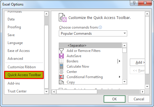
- Click File >Options >Quick Access Toolbar.
- Right-click anywhere on the ribbon and select Customize Quick Access Toolbar… from the context menu.
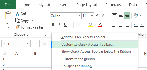
Click the Customize the Quick Access Toolbar button (the down arrow at the far-right of the QAT) and choose More Commands in the pop-up menu.
Whatever way you go, the Customize Quick Access Toolbar dialog window will open, where you can add, remove, and reorder the QAT commands. Below, you will find the detailed steps to do all the customizations. The guidelines are the same for all versions of Excel 2019, Excel 2016, Excel 2013 and Excel 2010.
How to add a command button to Quick Access Toolbar
Depending on what kind of command you’d like to add, this can be done in 3 different ways.
Enable a command from the predefined list
To enable a currently hidden command from the predefined list, this is what you need to do:
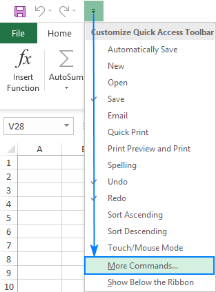
- Click the Customize Quick Access Toolbar button (the down arrow).
- In the list of the displayed commands, click the one you wish to enable. Done!
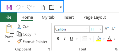
For example, to be able to create a new worksheet with a mouse click, select the New command in the list, and the corresponding button will immediately appear in the Quick Access Toolbar:
Add a ribbon button to Quick Access Toolbar
The fastest way to add to the QAT a command that appears on the ribbon is this:
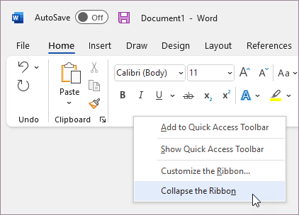
- Right-click the desired command on the ribbon.
- Select the Add to Quick Access Toolbar in the context menu.
Add a command that isn’t on the ribbon to Quick Access Toolbar
To add a button that is not available on the ribbon, carry out these steps:
- Right-click the ribbon and click Customize Quick Access Toolbar… .
- In the Choose commands from drop-down list on the left, select Commands Not in the Ribbon.
- In the list of commands on the left, click the command you want to add.
- Click the Add button.
- Click OK to save the changes.
For example, to have the ability to close all open Excel windows with a single mouse click, you can add the Close All button to the Quick Access Toolbar.
How to remove a command from Quick Access Toolbar
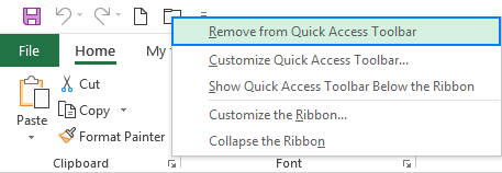
To remove either a default or custom command from the Quick Access Toolbar, right-click it and pick Remove from Quick Access Toolbar from the pop-up menu:
Or select the command in the Customize the Quick Access Toolbar window, and then click the Remove button.
Rearrange commands on Quick Access Toolbar
To change the order of the QAT commands, do the following:
- Open the Customize the Quick Access Toolbar window.
- Under Customize Quick Access Toolbar on the right, select the command that you want to move, and click the Move Up or Move Down arrow.
For example, to move the New File button to the far-right end of the QAT, select it and click the Move Down arrow.
Group commands on Quick Access Toolbar
If your QAT contains quite a lot of commands, you may want to sub-divide them into logical groups, for instance, separating the default and custom commands.
Though the Quick Access Toolbar does not allow creating groups like on the Excel ribbon, you can group commands by adding a separator. Here’s how:
- Open the Customize the Quick Access Toolbar dialog window.
- In the Choose commands from drop-down list on the left, pick Popular Commands.
- In the list of commands on the left, select and click Add.
- Click the MoveUp or MoveDown arrow to position the separator where needed.
- Click OK to save the changes.
As the result, the QAT appears to have two sections:
Add macros to Quick Access Toolbar in Excel
To have your favorite macros at your fingertips, you can add them to the QAT too. To have it done, please follow these steps:
- Open the Customize the Quick Access Toolbar window.
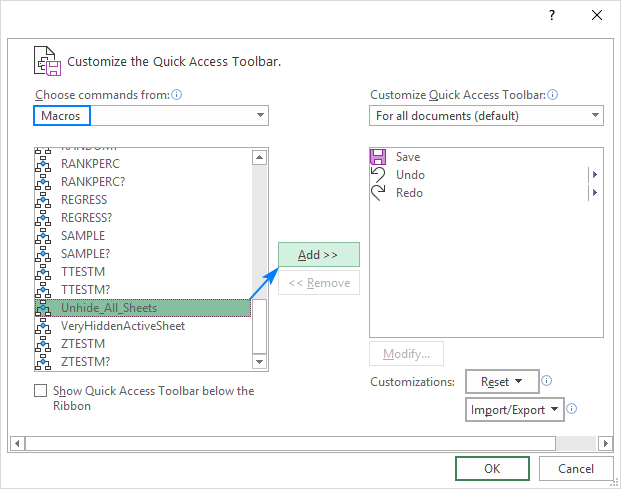
- In the Choose commands from drop-down list on the left, select Macros.
- In the list of macros, select the one you wish to add to the Quick Access Toolbar.
- Click the Add button.
- Click OK to save the changes and close the dialog box.
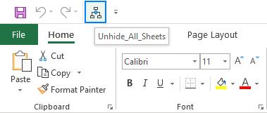
As an example, we are adding a custom macro that unhides all sheets in the current workbook:
Optionally, you can put a separator before the macro like shown in the screenshot below:
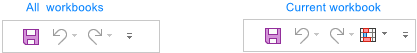
By default, the Quick Access Toolbar in Excel is customized for all workbooks.
If you’d like to make certain customizations for the active workbook only, select the current saved workbook from the Customize Quick Access Toolbar drop-down list, and then add the commands you want.
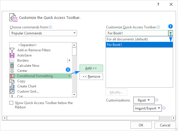
Please note that the customizations made for the current workbook do not replace the existing QAT commands but are added to them.
For example, the Conditional Formatting button that we have added for the current workbook appears after all other commands on the Quick Access Toolbar:
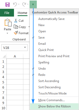
The default location of the Quick Access Toolbar is at the top of the Excel window, above the ribbon. If you find it more convenient to have the QAT below the ribbon, here’s how you can move it:
- Click the Customize Quick Access Toolbar button.
- In the pop-up list of options, select Show Below the Ribbon.
To get the QAT back to the default location, click the Customize Quick Access Toolbar button again, and then click Show Above the Ribbon.
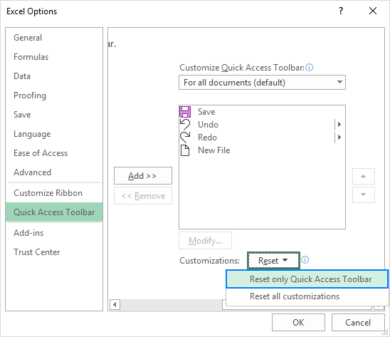
If you wish to discard all your customizations and revert the QAT back to its original setup, you can reset it in this way:
- Open the Customize the Quick Access Toolbar window.
- Click the Reset button, and then click Reset only Quick Access Toolbar.
Microsoft Excel allows saving your Quick Access Toolbar and ribbon customizations into a file that can be imported later. This can help you keep your Excel interface looking the same on all the computers that you use as well as share your customizations with your colleagues.
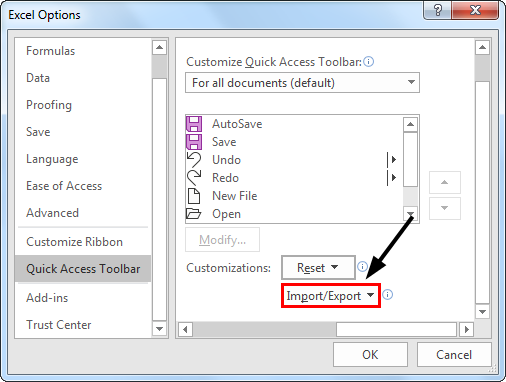
- Export a customized QAT:
In the Customize the Quick Access Toolbar window, click Import/Export, then click Export all customizations, and save the customizations file to some folder.
Import a customized QAT:
In the Customize the Quick Access Toolbar window, click Import/Export, select Import customization file, and browse for the customizations file that you saved earlier.
- The file that you export and import also includes the ribbon customizations. Unfortunately, there is no easy way to export or import only the Quick Access Toolbar.
- When you import the customizations file to a given PC, all prior ribbon and QAT customizations on that PC are permanently lost. To be able to restore your current customizations in the future, be sure to export them and save as a backup copy before importing any new customizations.
That’s how you customize and use the Quick Access Toolbar in Excel. I thank you for reading and hope to see you on our blog next week!
Источник
If the toolbar is not showing in Excel, the ribbon shortcut makes it visible.
by Vlad Turiceanu
Passionate about technology, Windows, and everything that has a power button, he spent most of his time developing new skills and learning more about the tech world. Coming… read more
Updated on February 9, 2023
Reviewed by
Alex Serban

After moving away from the corporate work-style, Alex has found rewards in a lifestyle of constant analysis, team coordination and pestering his colleagues. Holding an MCSA Windows Server… read more
- If your Excel toolbar disappeared, that is because you probably enabled it by mistake.
- As a preliminary check, you can try the simple command mentioned in the article.
- If it didn’t work for you, the guide below will show you what to do to unhide the excel menu bar when missing.
XINSTALL BY CLICKING THE DOWNLOAD FILE
This software will repair common computer errors, protect you from file loss, malware, hardware failure and optimize your PC for maximum performance. Fix PC issues and remove viruses now in 3 easy steps:
- Download Restoro PC Repair Tool that comes with Patented Technologies (patent available here).
- Click Start Scan to find Windows issues that could be causing PC problems.
- Click Repair All to fix issues affecting your computer’s security and performance
- Restoro has been downloaded by 0 readers this month.
Microsoft Excel is one of the most sophisticated tools in the Office suite, and it comes with loads of functions, most of which are manipulated using the toolbar. The toolbar missing makes it tough to get work done with Excel.
Without these crucial elements in Excel, you won’t be able to get jobs done quickly, so, understandably, you are searching for fixes.
The missing or hidden toolbar in Excel is a common complaint, but this is not usually a bug or issue from Excel itself. Incorrect display settings commonly cause it. Learn how to get your toolbar back in Excel.
Preliminary check:
➡️ Press CTRL + F1, which is the ribbon shortcut.
Pressing the ribbon button when the toolbar is visible hides it. If the toolbar is not showing in Excel, the ribbon shortcut makes it visible.
- How to show the toolbar in Excel?
- 1. Ribbon hidden, show the ribbon
- ✅ How to get toolbar back in Excel in 2 clicks
- 2. If the add-in tab is not showing in Excel
- 3. Other solutions for when Excel toolbars are missing
1. Ribbon hidden, show the ribbon
✅ How to get toolbar back in Excel in 2 clicks
This is a simple process that will unhide the toolbar. Be sure you follow the steps below:
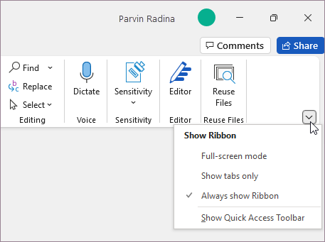
- In an MS Excel window, click on the Ribbon Display Options icon to reveal the following options:
- Auto-hide Ribbon:
- The ribbon disappears when you work on the sheet and shows up only when you hit ALT or click on the More ellipse icon.
- Show Tabs:
- Display only the tabs and leave the toolbar and ribbon hidden.
- Show Tabs and Commands:
- Display the tabs and commands at all times.
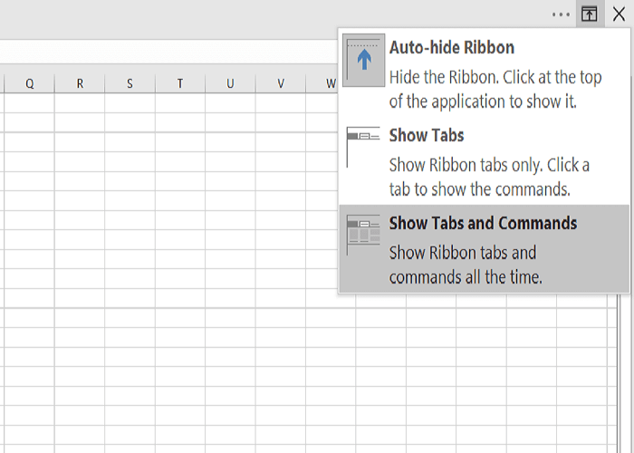
2. Select either Show Tabs or Show Tabs and Commands to display your toolbar to show the missing Excel toolbar.
2. If the add-in tab is not showing in Excel

- Hit the File menu link at the top of the page.
- From the File menu, select Options.
- Next, navigate to the Add-ins section from the left panel and select Disabled Items.
- If Excel disables the add-in, you will find it on the list here.
- Select the add-ins for which its tab is missing and hit Enable.
- Excel Running Slow? 4 Quick Ways to Make It Faster
- Fix: Excel Stock Data Type Not Showing
- Best Office Add-Ins: 15 Picks That Work Great in 2023
3. Other solutions for when Excel toolbars are missing
➡️Click on a tab to view the ribbon temporarily. Then, to the lower right of the screen, click the pin icon to pin the ribbon to the screen permanently.
➡️Double-click on the visible tab names.
➡️Right-click the tab and uncheck Collapse the Ribbon (or Minimize the Ribbon, depending on your Excel version).
➡️If you select the option of Auto-hide Ribbon, while working on the sheet, the ribbon and toolbar disappear. To see them, simply move your mouse to the top of the workbook and click.
Note that the above items are not steps to resolve the toolbar not showing in Excel issue; they are rather individual solutions that can help you get your toolbar back in Excel. Also, you can try them in any order.
The ribbon or toolbar is not showing in Excel is rarely a sign of an issue or bug; it is mostly due to the ribbon display settings. Press the ribbon shortcut (CTRL +F1) to show the Excel toolbar missing.
If that still does not solve the problem, then try out another solution on this page.
![]()
Newsletter
The name of the Quick Access Toolbar speaks for itself. Here are placed those tools, that the user uses most often. Moreover, here you can place tools that are not in the strip with bookmarks. For example, the «PivotTable Wizard», etc.
The Quick Access Toolbar – is the first best solution for users, who are migrating from older versions of Excel and do not have time to the learning of the new interface or its settings, but want to start working right away.
This panel is still useful in the mode of the folded main band of tools. Then there is not necessary to leave the convenient for viewing and working mode with folded strip each time.
Practical use of the Quick Access Toolbar
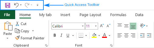
There is the Excel shortcut bar above of the wide tool bar. By default, there are 3 most frequently used tools:
- Save (CTRL + S).
- Cancel the input (CTRL + Z).
- Repeat input (CTRL + Y).
The amount of tools in the Quick Access Toolbar can be changed with using the setting.
- When downloading the program, the active cell on the blank sheet is located at A1 address. Type the letter «a» from the keyboard and press «Enter». The cursor will move down to the cell A2.
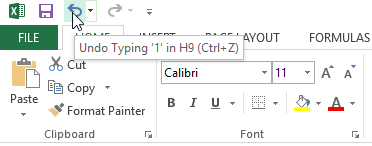
- Click the «Undo Input» tool (or the hotkey combination: CTRL + Z) and the text disappears, but the cursor returns to the starting position.
- If you perform to several actions on the worksheet (for example, fill in several letters with the letters), then the drop-down list of the action history for the «Cancel input» button will be available for you. Thus, you can cancel a lot of actions with one click, which is very convenient.
After of the canceling several actions, the history list for the «Repeat Input» tool is available.
Customize the Excel shortcut bar
The Quick Access Toolbar – is the flexible toolbar in Excel for simplifying and improving the user experience in the program.
You can place buttons of frequently used tools. Try adding the «Create» tool button yourself.
- On the right side, click on the drop-down list to call up the configuration options.
- From the list that appears, select the «New» option and add the tool for creating new Excel workbooks.
- Mark again the option «Create» from the list of settings to delete this tool.
The advanced Setup
In the panel setup options, using the drop-down list, only a few popular tools, but you can add to the panel any of tool available in Excel.
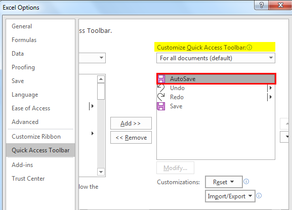
- To flexibly configure the contents of the Quick Access Toolbar, you must select the «Other Commands» option. The «Excel Options» window appears with the parameter «Quick Access Toolbar» already selected. To call this window you can and through the «File» option «Options», then select the necessary option.
- Select the tool in the left list, that you want to use often. Click on the «Add» button and press OK.
- To remove tools, select the tool from the right list and click on the «Delete» button, then OK.
Changing of the location
If necessary, this panel can be placed under the tool bar, not above it.
Open the drop-down list and select the «Place below the ribbon» option. This task can also be solved by using the context menu. To open the context menu, you need to right-click on the panel.
To return the panel back (by placing it over the tape), select the «Place over tape» option in the same way.
![]()
Written by Allen Wyatt (last updated December 3, 2018)
This tip applies to Excel 97, 2000, 2002, and 2003
As you are customizing Excel to reflect your working habits, there may be times when you want to create your own custom toolbar. You can create a toolbar by following these steps:
- Choose Customize from the Tools menu. This displays the Customize dialog box.
- Make sure the Toolbars tab is selected. (See Figure 1.)
- Click on New. This displays the New Toolbar dialog box. (See Figure 2.)
- Provide a name for your toolbar in the Toolbar Name box.
- Click on OK to close the New Toolbar dialog box. The toolbar appears at the bottom of the list of toolbars on the Toolbars tab of the Customize dialog box. The empty toolbar should also be visible on your screen.
- Click on the Commands tab in the Customize dialog box. (See Figure 3.)
- In the list of Categories, select the major category which contains the command you want to add to the new toolbar.
- In the list of Commands, select the command you want to add to the toolbar.
- Use the mouse to drag the command from the Commands list to its new location on your toolbar. When you release the mouse button, the icon or wording for the command appears.
- Repeat steps 7 through 9 to add more toolbar commands.
- Click on Close to dismiss the Customize dialog box.
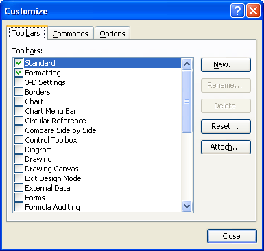
Figure 1. The Toolbars tab of the Customize dialog box.
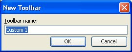
Figure 2. The New Toolbar dialog box.
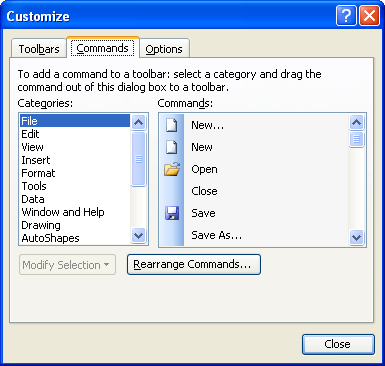
Figure 3. The Commands tab of the Customize dialog box.
ExcelTips is your source for cost-effective Microsoft Excel training.
This tip (2722) applies to Microsoft Excel 97, 2000, 2002, and 2003.
Author Bio
With more than 50 non-fiction books and numerous magazine articles to his credit, Allen Wyatt is an internationally recognized author. He is president of Sharon Parq Associates, a computer and publishing services company. Learn more about Allen…
MORE FROM ALLEN
Selecting Lots of Graphics
Need to select a lot of graphics in the document? Here’s an easy way to do it using tools available on the Drawing toolbar.
Discover More
Spell-Checking in a Protected Worksheet
When you protect a worksheet, you can’t use some tools, including the spell-checker. If you want to use it, you must …
Discover More
Calculating a Date Five Days before the First Business Day
Excel allows you to perform all sorts of calculations using dates. A good example of this is using a formula to figure …
Discover More
More ExcelTips (menu)
Changing Toolbar Location
Toolbars don’t need to be tethered to the top of your program window. Although they are right at home there, you may want …
Discover More
Resetting Toolbars to Their Default
Once you’ve edited your toolbars, you may want to change them back to their default appearance and behavior. This tip …
Discover More
Simplifying the Font List
Excel normally displays the font list on the toolbar or using the very fonts it is displaying. Here’s how to change that …
Discover More