About filters in excel - Word и Excel - помощь в работе с программами

Excel for Microsoft 365 Excel for Microsoft 365 for Mac Excel for the web Excel 2021 Excel 2021 for Mac Excel 2019 Excel for iPad Excel for iPhone Excel for Android tablets Excel for Android phones More…Less

The FILTER function allows you to filter a range of data based on criteria you define.

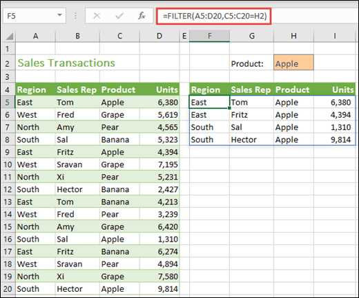
In the following example we used the formula =FILTER(A5:D20,C5:C20=H2,»») to return all records for Apple, as selected in cell H2, and if there are no apples, return an empty string («»).

The FILTER function filters an array based on a Boolean (True/False) array.

=FILTER(array,include,[if_empty])

Argument	Description
array Required	The array, or range to filter
include Required	A Boolean array whose height or width is the same as the array
[if_empty] Optional	The value to return if all values in the included array are empty (filter returns nothing)

Notes:

An array can be thought of as a row of values, a column of values, or a combination of rows and columns of values. In the example above, the source array for our FILTER formula is range A5:D20.
The FILTER function will return an array, which will spill if it’s the final result of a formula. This means that Excel will dynamically create the appropriate sized array range when you press ENTER. If your supporting data is in an Excel table, then the array will automatically resize as you add or remove data from your array range if you’re using structured references. For more details, see this article on spilled array behavior.
If your dataset has the potential of returning an empty value, then use the 3rd argument ([if_empty]). Otherwise, a #CALC! error will result, as Excel does not currently support empty arrays.
If any value of the include argument is an error (#N/A, #VALUE, etc.) or cannot be converted to a Boolean, the FILTER function will return an error.
Excel has limited support for dynamic arrays between workbooks, and this scenario is only supported when both workbooks are open. If you close the source workbook, any linked dynamic array formulas will return a #REF! error when they are refreshed.

Examples

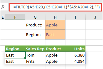
FILTER used to return multiple criteria

In this case, we’re using the multiplication operator (*) to return all values in our array range (A5:D20) that have Apples AND are in the East region: =FILTER(A5:D20,(C5:C20=H1)*(A5:A20=H2),»»).

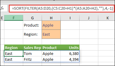
FILTER used to return multiple criteria and sort

In this case, we’re using the previous FILTER function with the SORT function to return all values in our array range (A5:D20) that have Apples AND are in the East region, and then sort Units in descending order: =SORT(FILTER(A5:D20,(C5:C20=H1)*(A5:A20=H2),»»),4,-1)

In this case, we’re using the FILTER function with the addition operator (+) to return all values in our array range (A5:D20) that have Apples OR are in the East region, and then sort Units in descending order: =SORT(FILTER(A5:D20,(C5:C20=H1)+(A5:A20=H2),»»),4,-1).

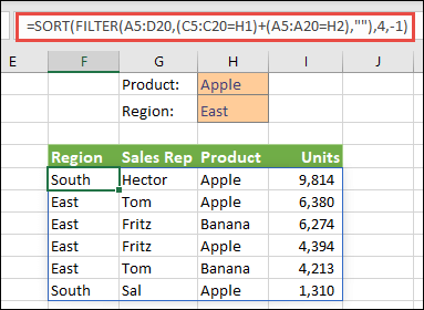
Notice that none of the functions require absolute references, since they only exist in one cell, and spill their results to neighboring cells.

Need more help?

You can always ask an expert in the Excel Tech Community or get support in the Answers community.

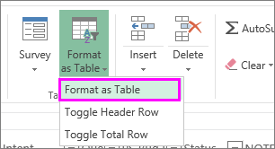
Select the data you want to filter. On the Home tab, click Format as Table, and then pick Format as Table.
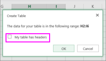
In the Create Table dialog box, you can choose whether your table has headers.
- Select My table has headers to turn the top row of your data into table headers. The data in this row won’t be filtered.
- Don’t select the check box if you want Excel for the web to add placeholder headers (that you can rename) above your table data.
Click OK.
To apply a filter, click the arrow in the column header, and pick a filter option.

Filter a range of data

If you don’t want to format your data as a table, you can also apply filters to a range of data.

Select the data you want to filter. For best results, the columns should have headings.
On the Data tab, choose Filter.

Filtering options for tables or ranges

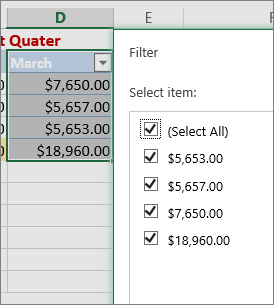
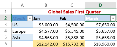
You can either apply a general Filter option or a custom filter specific to the data type. For example, when filtering numbers, you’ll see Number Filters, for dates you’ll see Date Filters, and for text you’ll see Text Filters. The general filter option lets you select the data you want to see from a list of existing data like this:

Number Filters lets you apply a custom filter:

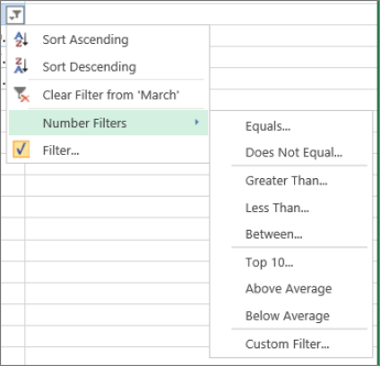
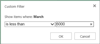
In this example, if you want to see the regions that had sales below $6,000 in March, you can apply a custom filter:

Here’s how:

Click the filter arrow next to March > Number Filters > Less Than and enter 6000.
Click OK.

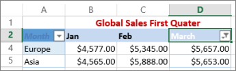
Excel for the web applies the filter and shows only the regions with sales below $6000.

You can apply custom Date Filters and Text Filters in a similar manner.

To clear a filter from a column

Click the Filter button next to the column heading, and then click Clear Filter from <«Column Name»>.

To remove all the filters from a table or range

Select any cell inside your table or range and, on the Data tab, click the Filter button.

This will remove the filters from all the columns in your table or range and show all your data.

Click a cell in the range or table that you want to filter.
On the Data tab, click Filter.
Click the arrow in the column that contains the content that you want to filter.
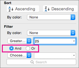
Under Filter, click Choose One, and then enter your filter criteria.

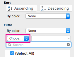
Notes:

You can apply filters to only one range of cells on a sheet at a time.
When you apply a filter to a column, the only filters available for other columns are the values visible in the currently filtered range.
Only the first 10,000 unique entries in a list appear in the filter window.

Click a cell in the range or table that you want to filter.
On the Data tab, click Filter.
Click the arrow in the column that contains the content that you want to filter.
Under Filter, click Choose One, and then enter your filter criteria.
In the box next to the pop-up menu, enter the number that you want to use.
Depending on your choice, you may be offered additional criteria to select:

Notes:

You can apply filters to only one range of cells on a sheet at a time.
When you apply a filter to a column, the only filters available for other columns are the values visible in the currently filtered range.
Only the first 10,000 unique entries in a list appear in the filter window.
Instead of filtering, you can use conditional formatting to make the top or bottom numbers stand out clearly in your data.

You can quickly filter data based on visual criteria, such as font color, cell color, or icon sets. And you can filter whether you have formatted cells, applied cell styles, or used conditional formatting.

In a range of cells or a table column, click a cell that contains the cell color, font color, or icon that you want to filter by.
On the Data tab, click Filter .
Click the arrow in the column that contains the content that you want to filter.
Under Filter, in the By color pop-up menu, select Cell Color, Font Color, or Cell Icon, and then click a color.

This option is available only if the column that you want to filter contains a blank cell.

Click a cell in the range or table that you want to filter.
On the Data toolbar, click Filter.
Click the arrow in the column that contains the content that you want to filter.
In the (Select All) area, scroll down and select the (Blanks) check box.
Notes:
- You can apply filters to only one range of cells on a sheet at a time.
- When you apply a filter to a column, the only filters available for other columns are the values visible in the currently filtered range.
- Only the first 10,000 unique entries in a list appear in the filter window.

Click a cell in the range or table that you want to filter.
On the Data tab, click Filter .
Click the arrow in the column that contains the content that you want to filter.

Under Filter, click Choose One, and then in the pop-up menu, do one of the following:

To filter the range for	Click
Rows that contain specific text	Contains or Equals.
Rows that do not contain specific text	Does Not Contain or Does Not Equal.

In the box next to the pop-up menu, enter the text that you want to use.

Depending on your choice, you may be offered additional criteria to select:

To	Click
Filter the table column or selection so that both criteria must be true	And.
Filter the table column or selection so that either or both criteria can be true	Or.

Click a cell in the range or table that you want to filter.
On the Data toolbar, click Filter .
Click the arrow in the column that contains the content that you want to filter.

Under Filter, click Choose One, and then in the pop-up menu, do one of the following:

To filter for	Click
The beginning of a line of text	Begins With.
The end of a line of text	Ends With.
Cells that contain text but do not begin with letters	Does Not Begin With.
Cells that contain text but do not end with letters	Does Not End With.

In the box next to the pop-up menu, enter the text that you want to use.

Depending on your choice, you may be offered additional criteria to select:

To	Click
Filter the table column or selection so that both criteria must be true	And.
Filter the table column or selection so that either or both criteria can be true	Or.

Wildcard characters can be used to help you build criteria.

Click a cell in the range or table that you want to filter.
On the Data toolbar, click Filter.
Click the arrow in the column that contains the content that you want to filter.
Under Filter, click Choose One, and select any option.
In the text box, type your criteria and include a wildcard character.

For example, if you wanted your filter to catch both the word «seat» and «seam», type sea?.

Do one of the following:

Use	To find
? (question mark)	Any single character For example, sm?th finds «smith» and «smyth»
* (asterisk)	Any number of characters For example, *east finds «Northeast» and «Southeast»
~ (tilde)	A question mark or an asterisk For example, there~? finds «there?»

Use

To find

? (question mark)

Any single character

For example, sm?th finds «smith» and «smyth»

* (asterisk)

Any number of characters

For example, *east finds «Northeast» and «Southeast»

~ (tilde)

A question mark or an asterisk

For example, there~? finds «there?»

Do any of the following:

To	Do this
Remove specific filter criteria for a filter	Click the arrow in a column that includes a filter, and then click Clear Filter.
Remove all filters that are applied to a range or table	Select the columns of the range or table that have filters applied, and then on the Data tab, click Filter.
Remove filter arrows from or reapply filter arrows to a range or table	Select the columns of the range or table that have filters applied, and then on the Data tab, click Filter.

When you filter data, only the data that meets your criteria appears. The data that doesn’t meet that criteria is hidden. After you filter data, you can copy, find, edit, format, chart, and print the subset of filtered data.

Table with Top 4 Items filter applied

Filters are additive. This means that each additional filter is based on the current filter and further reduces the subset of data. You can make complex filters by filtering on more than one value, more than one format, or more than one criteria. For example, you can filter on all numbers greater than 5 that are also below average. But some filters (top and bottom ten, above and below average) are based on the original range of cells. For example, when you filter the top ten values, you’ll see the top ten values of the whole list, not the top ten values of the subset of the last filter.

In Excel, you can create three kinds of filters: by values, by a format, or by criteria. But each of these filter types is mutually exclusive. For example, you can filter by cell color or by a list of numbers, but not by both. You can filter by icon or by a custom filter, but not by both.

Filters hide extraneous data. In this manner, you can concentrate on just what you want to see. In contrast, when you sort data, the data is rearranged into some order. For more information about sorting, see Sort a list of data.

When you filter, consider the following guidelines:

Only the first 10,000 unique entries in a list appear in the filter window.
You can filter by more than one column. When you apply a filter to a column, the only filters available for other columns are the values visible in the currently filtered range.
You can apply filters to only one range of cells on a sheet at a time.

Note: When you use Find to search filtered data, only the data that is displayed is searched; data that is not displayed is not searched. To search all the data, clear all filters.

Need more help?

You can always ask an expert in the Excel Tech Community or get support in the Answers community.

Источник

What is Filter in Excel?

The filter in excel helps display relevant data by eliminating the irrelevant entries temporarily from the view. The data is filtered as per the given criteria. The purpose of filtering is to focus on the crucial areas of a dataset. For example, the city-wise sales data of an organization can be filtered by the location. Hence, the user can view the sales of selected cities at a given time.

A filter is necessarily required when working with a huge database. Being a widely used tool, the filter converts a comprehensive view into an easy-to-understand one. To apply filters, the dataset must contain a header row which specifies the name of every column.

What is Filter in Excel?
- How to Filter in Excel?
  - Method 1: With Filter Option Under the Home tab
  - Method 2: With Filter Option Under the Data tab
  - Method 3: With the Shortcut key
- How to Add Filters in Excel?
  - Example #1–“Number Filters” Option
  - Example #2–“Search Box” Option
- Option while you Drop Down the Filter Function
- The Techniques of Filtering in Excel
- Frequently Asked Questions
- Recommended Articles

How to Filter in Excel?

You can download this Filter Column Excel Template here – Filter Column Excel Template

It is good to work with filters because they fit our needs the way we want to. In order to filter data, select the entries to be visible and deselect the rest of the items.

The three methods to add filters in excel are listed as follows:

With filter option under the Home tab
With filter option under the Data tab
With the shortcut key

Let us consider a dataset to go through the three methods of adding filters.

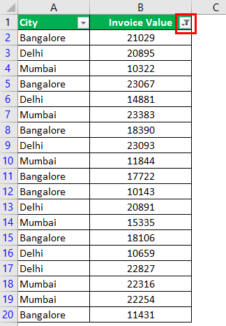
The following table shows the invoices issued to the buyers of different cities. We want to filter the data using different methods.

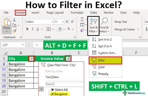
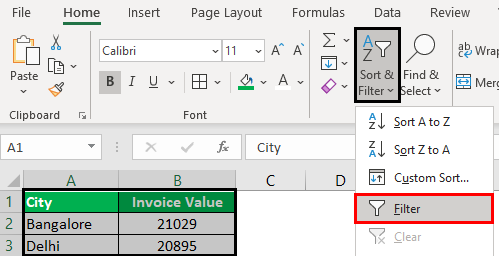
Method 1: With Filter Option Under the Home tab

In the Home tab, there is a “filter” option under the “sort and filter” drop-down of the “editing” section, as shown in the following image.

Step 1: Select the data and click “filter” under the “sort and filter” drop-down.

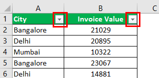
Step 2: The filters are added to the selected data range. The drop-down arrows, shown within the red boxes in the following image, are filters.

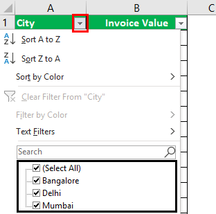
Step 3: Click the drop-down arrow of the column “city” to view the different names of the cities.

Step 4: To see the invoice values of “Delhi” only, select “Delhi” and uncheck all the remaining boxes.

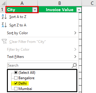
Step 5: The data for the city “Delhi” is filtered and displayed in the following image.

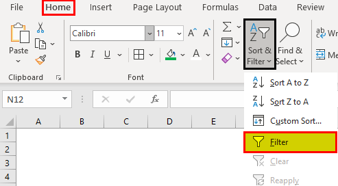
Method 2: With Filter Option Under the Data tab

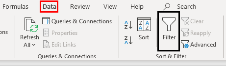
In the Data tab, there is a “filter” option under the “sort and filter” section, as shown in the following image.

Method 3: With the Shortcut key

The keyboard shortcutsAn Excel shortcut is a technique of performing a manual task in a quicker way.read more are a good way to speed up the daily tasks. Select the data and add the filter using either of the following shortcuts:

Press the keys “Shift+Ctrl+L” together.

Press the keys “Alt+D+F+F” together.

Note: The preceding shortcuts for adding filtersUsing sorting and filtering, we can see the data category wise. With filtering data quickly you can easily navigate through menus or clicking through a mouse in less time.read more are toggle keys. Repetitive pressing helps to turn on and turn off the filters.

How to Add Filters in Excel?

We can filter numbers using advanced techniques. Let us consider some examples to understand the working of filters in Excel.

Example #1–“Number Filters” Option

Working on the data under the preceding heading (methods of filtering in Excel), we want to apply the following filters:

a. To filter column B (invoice value) for numbers greater than 10000

b. To filter column B for numbers greater than 10000 but less than 20000

Let us go through the two cases one by one.

a. Filter numbers greater than 10000

Step 1: Open the filter in column B (invoice value) by clicking on the filter symbol.

Step 2: In “number filters,” choose the “greater than” option, as shown in the following image.

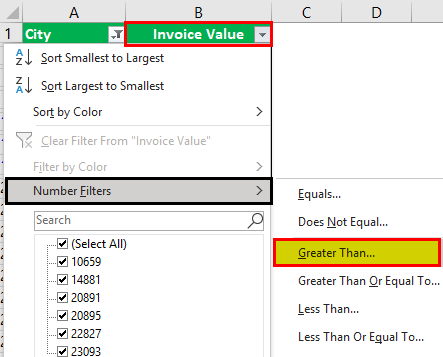
Step 3: The “custom autofilter” box appears.

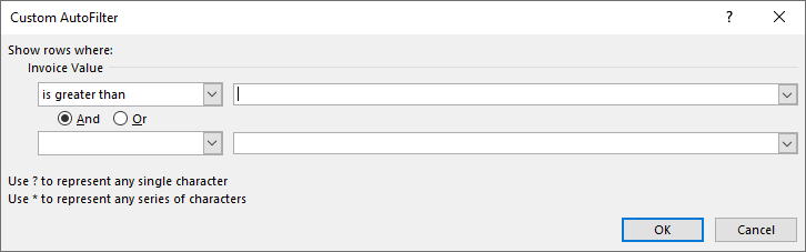
Step 4: Enter the number 10000 in the box to the right of “is greater than.”

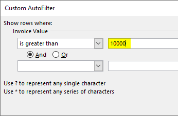
Step 5: The output displays the invoice values greater than 10000. The symbol within the red box is the filter icon. It indicates that the filter has been applied to column B.

b. Filter numbers greater than 10000 but less than 20000

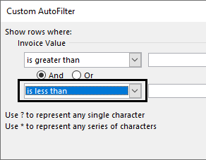
Step 1: In “number filters,” choose the “greater than” option.

Step 2: In the “custom autofilter” box, select “is less than” in the second box to the left-hand side. This is shown in the following image.

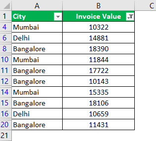
Step 3: Enter the number 10000 in the box to the right of “is greater than.” Enter the number 20000 in the box to the right of “is less than.”

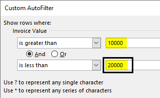
Step 4: The output displays the invoice values greater than 10000 but less than 20000.

Example #2–“Search Box” Option

Working on the data under the preceding heading (methods of filtering in Excel), we have replaced the first column (city) with product IDs.

We want to filter the details of product ID “prd 1.”

The steps are listed as follows:

Step 1: Add filters to the columns “product ID” and “invoice value.”

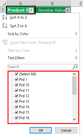
Step 2: In the search boxA search box in Excel finds the needed data by typing into it, then filters the data and displays only that much info. When working with large datasheets, this simple tool may save a lot of time.read more, enter the value that is to be filtered. So, enter “prd 1.”

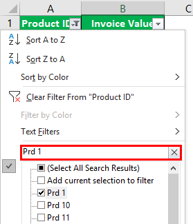
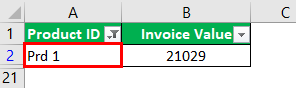
Step 3: The output displays only the filtered value from the list, as shown in the following image. Hence, we can see the invoice value of the product ID “prd 1.”

Option while you Drop Down the Filter Function

Sort A to Z and Sort Z to A: If you wish to arrange your data ascending or descending order.
Sort by Color: If you want to filter the data by color if a cell is filled by color.
Text filter: When you want to filter a column with some exact text or number.
Filter cells that begin with or end with an exact character or the text
Filter cells that contain or do not contain a given character or word anywhere in the text.
Filter cells that are exactly equal or not equal to a detailed character.

For example:

Suppose you want to use the filter for a specific item. Click on to text filter and choose equals.

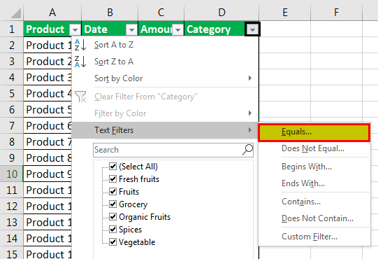
It enables you the one dialogue, which includes a Custom Auto-Filter dialogue box.

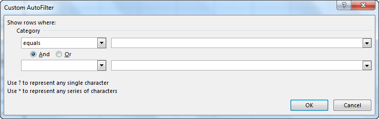
Enter fruits under category and click Ok.

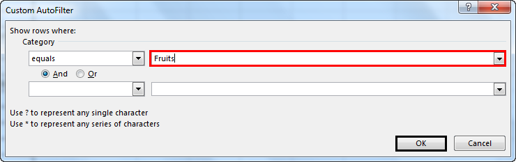
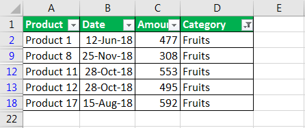
Now you will get the data of fruits category only as shown below.

The Techniques of Filtering in Excel

The following techniques must be followed while filtering data:

If the dataset is large, type the value to be filtered. This filters all the possible matches.
If numerical data has to be filtered by specifying the greater than or the less than number, use the “number filters” option.
If data has to be filtered by the color of specific rows, use the “filter by color” option.

Frequently Asked Questions

1. What are filters and how to add them in Excel?

Filtering is a technique which displays the required information and removes the unwanted data from the view. It helps the user focus on the relevant data at a given time.

The steps to add filters in Excel are listed as follows:
• Ensure that a header row appears on top of the data, specifying the column labels.
• Select the data on which filters are to be added.
• Add filters by any of the three given methods.
o Click the “filter” option under the “sort and filter” (editing section) drop-down of the Home tab.
o Click the “filter” option under the “sort and filter” section of the Data tab.
o Press the keys “Shift+Ctrl+L” or “Alt+D+F+F.”

Note: As soon as the filters are added, a drop-down arrow appears on the particular column header.

2. How to apply filters to one or more columns?

The steps to apply filters to one or more columns are listed as follows:
• Click the drop-down arrow of the column to be filtered.
• Uncheck the “select all” option which helps deselect all data.
• Select the boxes to be displayed.
• Click “Ok.”
The drop-down arrow changes to the filter icon as soon as a filter is applied. When filters are applied to multiple columns, the filter icon appears on each one of them. Hovering over the filter icon shows the filters that have been applied.

Note: The drop-down arrow on a column header indicates a filter is added. The filter icon indicates a filter has been applied.

3. How to use filters in Excel?

The filters can be applied to numbers, text values, and dates. These cases are discussed as follows:
Filter numbers
• Click on the “number filters.”
• Select any of the options like “equals,” “does not equals,” “greater than,” “less than,” “between,” “above average,” and so on.
• Specify the required fields in the dialog box that appears. This box may or may not be displayed.

For instance, in “equals,” enter the number against which the values should be compared. The filtered results show the matching numerical values.

Filter text and date values
• To filter text and date values, select “text filters” and “date filters” from the respective drop-down arrows.
• The “text filters” allow filtering text strings which contain specific characters or words. The “date filters” allow filtering dates for a particular year, month, week, and so on.

Note: The “plus” and the “minus” sign of the date filters are used for expanding and collapsing the various levels respectively.

Here are the Excel Filters formulas:

Filter by a number

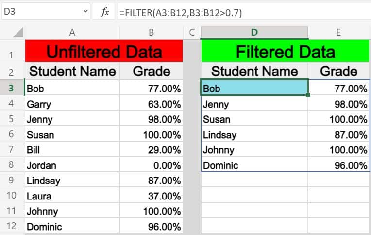
=FILTER(A3:B12, B3:B12>0.7)

Filter by a cell value

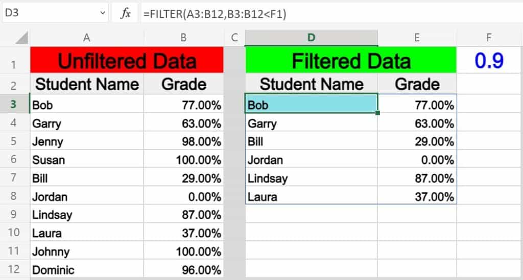
=FILTER(A3:B12, B3:B12<F1)

Filter by a text string

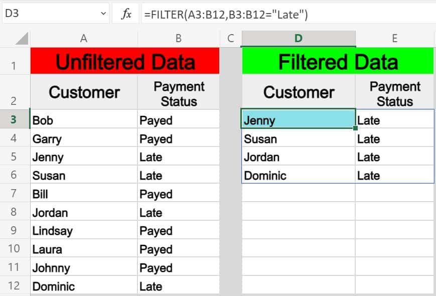
=FILTER(A3:B12, B3:B12=»Late»)

Filter where NOT equal to

=FILTER(A3:E1000, B3:B1000<>»Bob»)

Filter by date

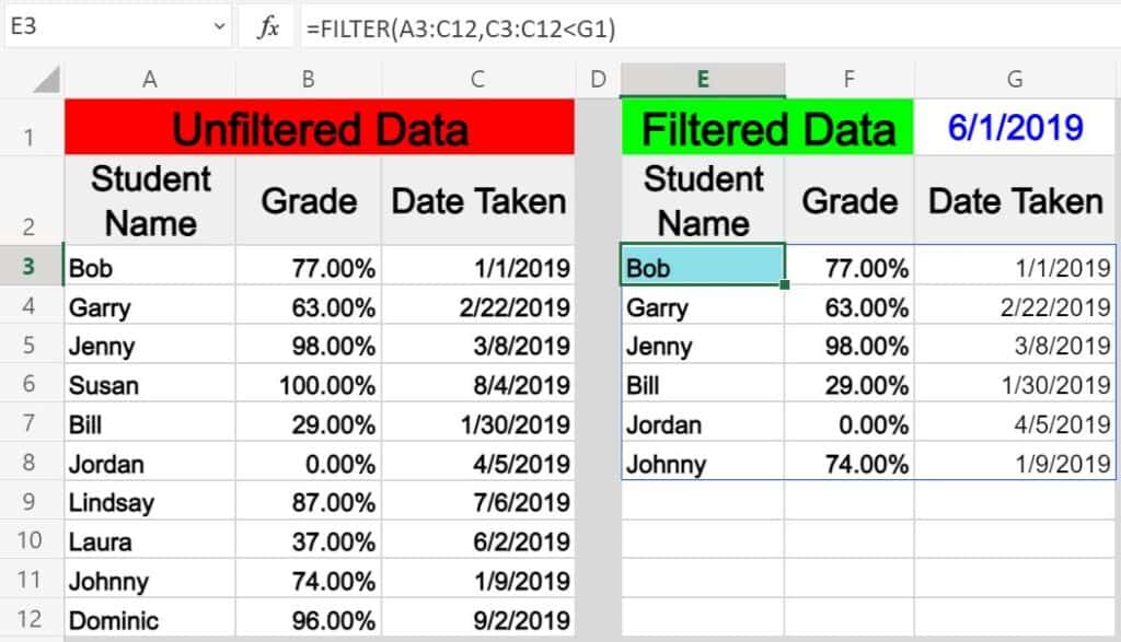
=FILTER(A3:C12,C3:C12<G1) (Date entered in cell G1)
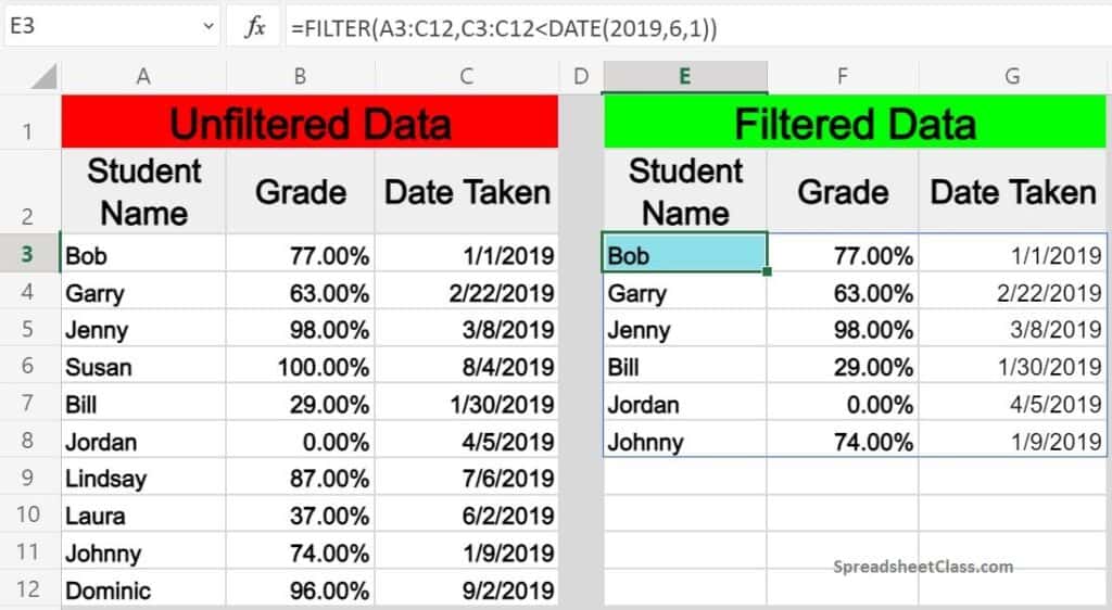
=FILTER(A3:C12,C3:C12<DATE(2019,6,1))

Filter by multiple conditions

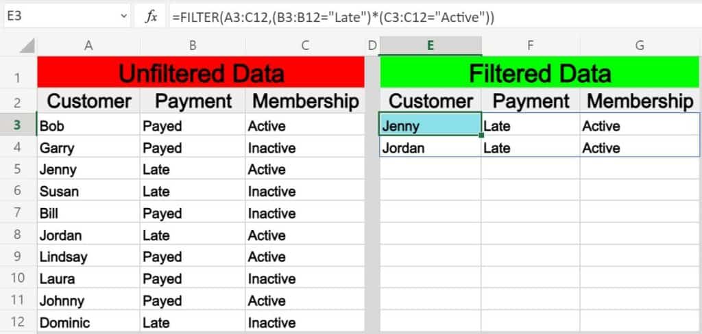
=FILTER(A3:C12,(B3:B12=»Late»)*(C3:C12=»Active»)) (AND logic)
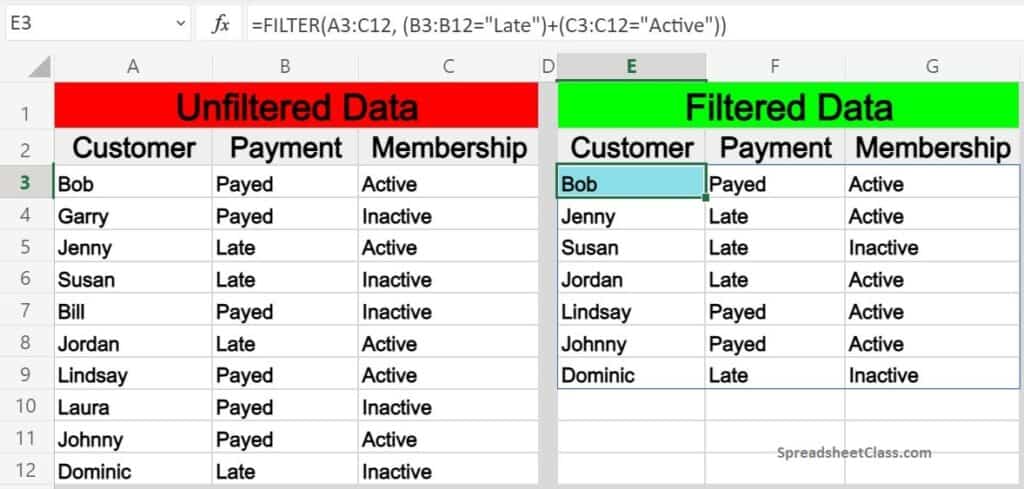
=FILTER(A3:C12, (B3:B12=»Late»)+(C3:C12=»Active»)) (OR logic)

Filter from another sheet

=FILTER(‘Sheet Name’!A3:B12,’Sheet Name’!B3:B12=»Full Time»)

=FILTER(A3:B12, B3:B12=F1)

(Copy/Paste the formula above into your sheet and modify as needed)

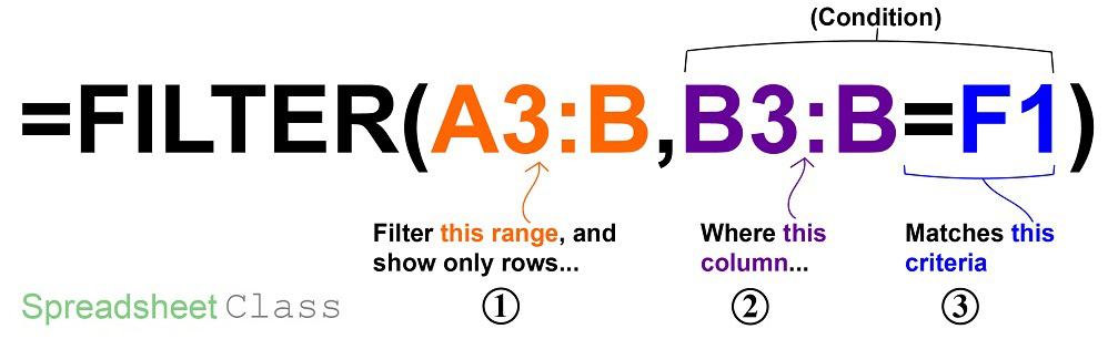
The FILTER function in Excel allows you to filter a range of data by a specified condition, so that a new set of data will be displayed which only shows the rows/columns from the original data set that meets the criteria/condition set in the formula.

Excel description for FILTER function:

Syntax:
=FILTER(array,include,[if_empty])

Formula summary: “The FILTER function filters an array based on a Boolean (True/False) array.”

array (Required): The array, or range to filter

include (Required): A Boolean array whose height or width is the same as the array

[if_empty] (Optional): The value to return if all values in the included array are empty (filter returns nothing)

The source range that you want to filter, can be a single column or multiple columns.

The range that is used to check against the criteria that you set, must be a single column (later I will show you how to filter by multiple conditions, but don’t worry about that for now).

The criteria that set in the condition can be manually typed into the formula as a number or text, or it can also be a cell reference.

*Note that the source range and the single column range for the condition, must be the same size (must contain the same number of rows), or the cell will display an error.

Filtering by a single condition in Excel

First let’s go over using the FILTER function in Excel in its simplest form, with a single condition/criteria.

I will show you how to filter by a number, a cell value, a text string, a date… and I will also show you how to use varying «operators» (Less than, Equal to, etc…) in the filter condition.

Part 1: How to filter by a number

In this first example on how to use the filter function in Excel, the scenario is that we have a list of students and their grades, and that we want to make a filtered list of only students who have a perfect grade.

The task: Show a list of students and their scores, but only those that have a perfect grade

The logic: Filter the range A3:B12, where the column B3:B12 is greater than 0.7 (70%)

The formula: The formula below, is entered in the blue cell (D3), for this example

=FILTER(A3:B12, B3:B12>0.7)

Operators that can be used in the FILTER function:

In this example we are using the operator «=» (Equal To) for the filter condition/criteria, but you can also use any of the following:

«=» (Equals)
«>» (Greater than)
«<» (Less than)
«<>» (Not equal to)
«>=» (Greater than or equal to)
«<=» (Less than or equal to)

Part 2: How to filter by a cell value in Excel

In this example, we want to achieve the same goal as discussed above, but rather than typing the condition that we want to filter by directly into the formula, we are using a cell reference.

When you filter by a cell value in Excel, your sheet will be setup so that you can change the value in the cell at any time, which will automatically update the value that the filter criteria it attached to.

In this example, you will notice that instead of directly typing the number “0.9” into the formula itself, the filter criteria is set as cell G1, where the “0.9” value is entered.

The task: Show a list of students and their scores, but only those that have a score below 90%

The logic: Filter the range A3:B12, where B3:B12 is less than the value that is entered in the cell F1 (0.9)

The formula: The formula below, is entered in the blue cell (D3), for this example

=FILTER(A3:B12, B3:B12<F1)

Part 3: How to filter by text in Excel

In this example, we are going to use a text string as the criteria for the filter formula. This is very similar to using a number, except that you must put the text that you want to filter by inside of quotation marks.

In this scenario we are filtering a list that shows customers and their payment status, and we want to display only customers that have a payment status of “Late”.

The task: Show a list of customers who are past due on their payments

The logic: Filter the range A3:B12, where B3:B12 equals the text, “Late”

The formula: The formula below, is entered in the blue cell (D3), for this example

=FILTER(A3:B12, B3:B12=»Late»)

Part 4: Using NOT EQUAL TO in the Excel FILTER function

Now that you have got a basic understanding of how to use the filter function in Excel, here is another example of filtering by a string of text, but in this example we will use the «not equal» operator (<>), so that you can learn how to filter a range and output data that is NOT equal to criteria that you specify.

In this example we will also use a larger data set to demonstrate a more extensive application of the FILTER function in the real world.

You may be surprised at how often a situation comes up when you need to filter data where it is “not equal to” a certain number or piece of text that you specify.

In this example let’s say that we have a report/spreadsheet that shows data from sales calls that occur at your company, and we want to filter the data so that a specified sales rep (Bob) is NOT included in the filter output.

The task: Show sales call data for all sales reps, except Bob

The logic: Filter the range A2:E1000, where B2:B1000 DOES NOT equal the text, “Bob”

The formula: The formula below, is entered in the blue cell (G3), for this example

=FILTER(A3:E1000, B3:B1000<>»Bob»)

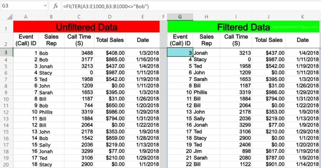
Notice that the filtered data on the right side of the image above does not contain any of the rows/calls that Bob was involved in.

Part 4: How to filter by date in Excel

Filtering by a date in Excel can be done in a couple of ways, which I will show you below. If you try to type a date into the FILTER function like you normally would type into a cell… the formula will not work correctly.

So you can either type the date that you want to filter by into a cell, and then use that cell as a reference in your formula… or you can use the DATE function.

When filtering by date you can use the same operators (>, <, =, etc…) as in other FILTER function applications. In Excel each different day/date is simply a number that is put into a special visual format. For example, in Excel, the date «06/01/2019» is simply the number «43,617», but displayed in date format. When you add one day to the date, this number increments by one each time… i.e «43,618» «43,619» «43,620»

So, one date can be considered to be «greater than» another date, if it is further in the future. Conversely, one date can be said to be «less than» another date, if it is further in the past.

In this first example we will filter by a date by using a cell reference. This is similar to the example we went over in part 2, but in this example instead of working with percentages, we are dealing with dates.

Let’s say that we want to filter a list of students, their test scores, and the dates that the tests were completed… and we want to show only tests that were taken before June (06/01/2019).

Filter by date in Excel example 1:

The task: Show only tests that were taken before June

The logic: Filter the range A3:C12, where C3:C12 is less than the date that is entered in cell G1 (06/01/2019)

The formula: The formula below, is entered in the blue cell (E3), for this example

=FILTER(A3:C12,C3:C12<G1)

Filter by date in Excel example 2:

In this second example on filtering by date in Excel we are using the same data as above, and trying to achieve the same results… but instead of using a cell reference, we will use the DATE function so that you can type enter the date directly into the FILTER function.

When using the DATE function to designate a certain date, you must first enter the year, then the month, and then the day… each separated by commas (shown below).

The task: Show only tests that were taken before June

The logic: Filter the range A3:C12, where C3:C12 is less than the date of (06/01/2019)

The formula: The formula below, is entered in the blue cell (E3), for this example

=FILTER(A3:C12,C3:C12<DATE(2019,6,1))

Filter by multiple conditions in Excel

When using the Excel FILTER function you may want to output a set of data that meets more than just one criteria. I will show you two ways to filter by multiple conditions in Excel, depending on the situation that you are in, and depending on how you want to formula to operate.

The normal way of adding another condition to your filter function, (as shown by the formula syntax in Excel), will allow you to set a second condition, where the first AND second condition must be met to be returned in filter output.

However I will also show you how to make a slight modification to the function so that you can choose to set a second condition where EITHER condition can be met to return/display in the filter function’s output/destination. (Separate the conditions with an asterisk to use AND logic, or separate the conditions with a plus sign to use AND logic.)

Part 5: Filtering by 2 conditions where BOTH MUST BE TRUE

In this example, we are going to filter a set of data, and only display rows where BOTH the first condition AND the second condition are met/true.

To use a second condition in this way (with AND logic), simply enter the second condition into the formula after the first condition, separated by an asterisk (*). Each condition must be inside of its own set of parenthesis (shown below).

When using the filter formula with multiple conditions like this, the columns that are referenced in each condition must be different.

In this scenario we want to filter a list that shows customers, their payment status, and their membership status… and to show only customers who have an active membership AND who are also late on their payment.

This will make sure that customers with an inactive membership who are still designated as being late on payment in the system… are not shown in the filter results, and not put on the list for being sent a «late payment» notice.

The task: Show a list of customers who are late on their payments, but only those with active memberships

The logic: Filter the range A3:C12, where B3:B12 equals the text “Late”, AND where C3:C12 equals the text “Active”

The formula: The formula below, is entered in the blue cell (E3), for this example

=FILTER(A3:C12,(B3:B12=»Late»)*(C3:C12=»Active»))

Part 6: Filtering by 2 conditions where EITHER ARE TRUE, not necessarily both

In this example we are going to filter a set of data and only display rows where EITHER the first condition OR the second condition are met/true.

To use a second condition in this way (with OR logic), simply enter the second condition into the formula after the first condition, separated by a plus sign. Each condition must be inside of its own set of parenthesis (shown below).

When using the FILTER formula in this way, you can choose criteria from the same or different columns.

In this scenario we want to filter the same customer data as shown in the previous example, but this time we want to show a list of customers who EITHER have an active membership OR who are late on their payment. This will give a list of customers who can be sent a notice for payment… including active members, or/also inactive members who are late on their final payment.

The task: Show a list of customers who are active members, and include customers who are late on payment even if they are not active members

The logic: Filter the range A3:C12, where B3:B12 equals the text “Late”, OR where C3:C12 equals the text “Active”

The formula: The formula below, is entered in the blue cell (E3), for this example

=FILTER(A3:C12, (B3:B12=»Late»)+(C3:C12=»Active»))

How to filter from another sheet in Excel

You may often find situations where you need to filter from another sheet in Excel, where your raw unfiltered data is on one tab, and your filter formula / filter output is on another tab.

This can be done by simply referring to a certain tab name when specifying the ranges in the filter. So where you would normally set a range like «A3:B», when referencing another sheet while filtering you specify the tab name by adding the tab name and an exclamation mark before the column/row portion of the range, like «TabName!A3:B»

However when the tab name has a space in it, it is necessary to use an apostrophe before and after the tab name, like ‘Tab Name’!A3:B.

Here is an example of how to filter data from another tab in Excel, where your filter formula will be on a different tab than the source range.

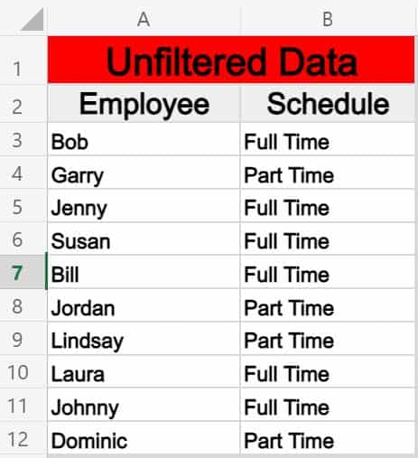
Let’s say that you have a list of employees and their schedule type (Full Time / Part Time) on one tab, and that you want to display a filtered list of full time employees on another tab.

The task: Filter the list of employees on the tab labeled «Filter List», and show a list of employees who have a full time schedule, on a separate tab

The logic: Filter the range ‘Filter List’!A3:B12, where the range ‘Filter List’!B3:B12 is equal to the text «Full Time»

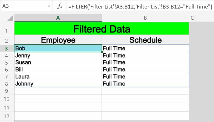
The formula: The formula below, is entered in the blue cell (A3), for this example

=FILTER(‘Filter List’!A3:B12,’Filter List’!B3:B12=»Full Time»)

Here is a list of employees and their schedules, which is held on a tab labeled «Filter List»

And here is a filtered list of employees who have full time schedules, where the filter formula and output data are held on a separate tab.

Pop Quiz: Test your knowledge

Answer the questions below about the Excel FILTER function, to refine your knowledge! Scroll to the very bottom to find the answers to the quiz.

Question #1

Which of the following formulas uses a «cell reference» in the filter condition?

=FILTER(A1:D15, B1:B15<0.6)
=FILTER(A2:C15, C2:C15=F1)
=FILTER(A1:P25, G1:G25=»Yes»)

Question #2

Which of the following formulas uses the «Not Equal» operator?

=FILTER(C1:T50, J1:J50>100)
=FILTER(A1:B75, B1:B75=»No»)
=FILTER(S1:Z100, T1:T100<>»True»)

Question #3

True or False: If the column(s) in the source range and the column in the filter condition are not the same size (if one has more rows than the other), the formula will not work, and will display an error.

True
False

Question #4

Which of the following formulas uses AND logic, where BOTH conditions must be met to satisfy the filter criteria?

=FILTER(C1:F20, (F1:F20=»Yes»)+(E1:E20=»Active»))
=FILTER(C1:F35, (F1:F35=»Yes»)*(E1:E35=»Active»))

Question #5

Which of the following formulas uses OR logic, where EITHER condition can be met to satisfy the filter criteria?

=FILTER(A1:K10, (K1:K10=»Yes»)*(J1:J10=»Active»))
=FILTER(A3:K33, (K3:K33=»Yes»)+(J3:J33=»Active»))

Answers to the questions above:

Question 1: 2

Question 2: 3

Question 3: 1

Question 4: 2

Question 5: 2

Источник

Advanced filter in Excel provides more opportunities for managing on data management spreadsheets. It is more complex in settings, but much more effective in action.

Using a standard filter, a Microsoft Excel user can solve not all of the tasks that are set. There is no visual display of the applied filtering conditions. It is not possible to apply more than two selection criteria. You can not filter the duplicate values to leave only unique records. And the criteria themselves are schematic and simple. The functionality of the extended filter is much richer. Let’s take a closer look at its possibilities.

How to make the advanced filter in Excel?

The advanced filter allows you to analysis data on an unlimited set of conditions. With this tool, the user can:

to specify more than two selection criteria;
to copy the result of filtering to another sheet;
to set the condition of any complexity with the helping of formulas;
to extract the unique values.

The algorithm for applying the extended filter is simple.

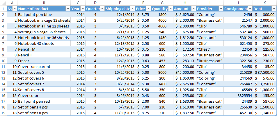
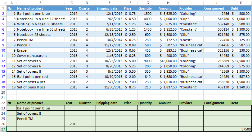
To make the table with the original data or to open an existing one. Like so:

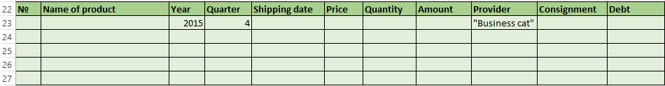
To create the condition table. The features: the header line is the same with the «cap» of the filtered table. To avoid errors, need to copy the header line in the source table and paste it on the same sheet (side, top, underarm) or on another sheet. We enter the selection criteria into the condition table.

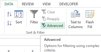
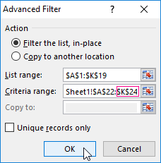
Go to the «DATA» tab — «Sort and filter» — «Advanced». If the filtered information should be displayed on another sheet (NOT where the source table is), then you need to run the extended filter from another sheet.

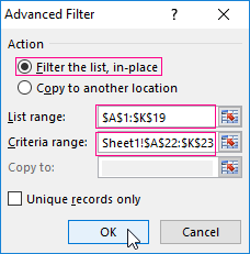
In the «Advanced Filter» window that opens, to select the method of processing information (on the same sheet or on the other one), set the initial range (the table 1, example) and the range of conditions (the table 2, conditions). The header lines must be included in the ranges.

ranges.

To close the «Advanced Filter» window, click OK. We see the result.

result.

The top table is the result of the filtering. The lower nameplate with the conditions is given for clarity near.

How to use the advanced filter in Excel?

To cancel the action of the advanced filter, we place the cursor anywhere in the table and press Ctrl + Shift + L or «DATA» — «Sort and Filter» — «Clear».

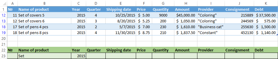
We will find using the «Advanced Filter» tool information on the values that contain the word «Set».

In the table of conditions we bring in the criteria. For example, these are:

The program in this case will search for all information on the goods, in the title of which there is the word «Set».

Set.

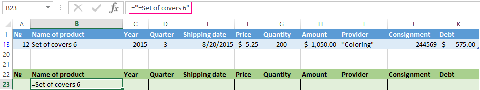
To search for the exact value, you can use the «=» sign. We enter the following criteria in the condition table:

Excel sees the «=» as a signal: the user will set the formula now. In order for the program to work correctly, the following should be written in the formula line: =»=Set of covers 6″.

After using the «Advanced Filter»:

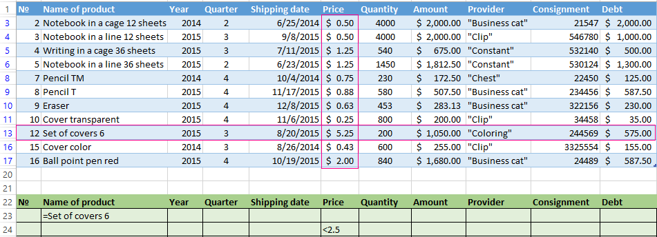
We filter the source table by the condition «OR» for different columns now. The operator «OR» is also in the tool «AutoFilter». But there it can be used within the single column.

In the condition label we introduce the selection criteria: =»=Set of covers 6″. (In the column «Name of product») and = «<2.5$» (in the column «Price»). That is, the program must select those values that contain the EXACTLY information about the good «Set of covers 6 ». OR to the information about the goods, which price is <2.5.

Please note: the criteria must be written under the corresponding headings in the DIFFERENT lines.

The result of selection:

The advanced filter allows you to use as a criterion of a formula. Let’s consider the example.

Selection of the line with the maximum indebtedness: =MAX(Table1[Debt]).

MAX.

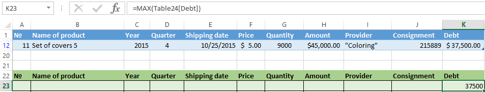
So we get the results as after running several filters on the one Excel sheet.

How to make few filters in Excel?

Let’s create the filter by several values. To do this, we enter in the table of conditions several criteria for selecting data:

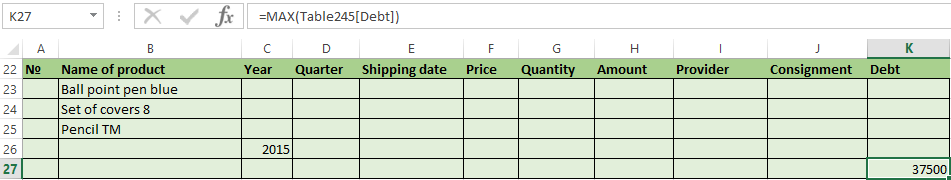
Apply the tool «Advanced Filter»:

Good.

Now from the table with the selected data we will extract new information, which was selected according to other criteria. There are only shipping date for autumn 2015 (from September to November). Example:

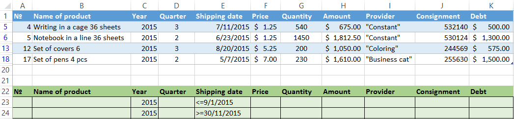
We introduce a new criterion in the condition table and apply the filtering tool. The initial range — is the table with data selected according to the previous criterion. This is how the filter is performed across on several columns.

To use few filters, you can create several condition tables on the new sheets. The method of implementation depends from the task which was set by user.

How to make the filter in Excel by lines?

By standard methods — you may not do it by any ways. Microsoft Excel selects data only in columns. Therefore, we need to look for other solutions.

Here are some examples of string criteria for the extended filter in Excel:

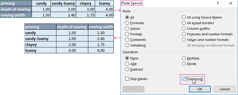
Convert to the table. For example, from three rows make a list of three columns and apply the filtering to the transformed version.

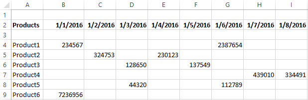
Use formulas to display exactly the data in the string that are needed. For example, make some indicator drop-down list. And in the next cell, enter the formula using the IF function. When a certain value is selected from the drop-down list, its parameter appears next to it.

To give an example of how the filter works by rows in Excel, we are creating the label:

For the list of products, we create the drop-down list:

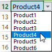
If necessary, learn how to create a drop-down list in Excel.

Above the table with the original data, we insert an empty line. In the cells, we introduce the formula that will show which columns the information is taken from.

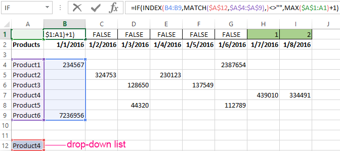
Next to the drop-down list box, we enter the following formula:

Its task is select from the table those values, that correspond to a certain good.

Done.

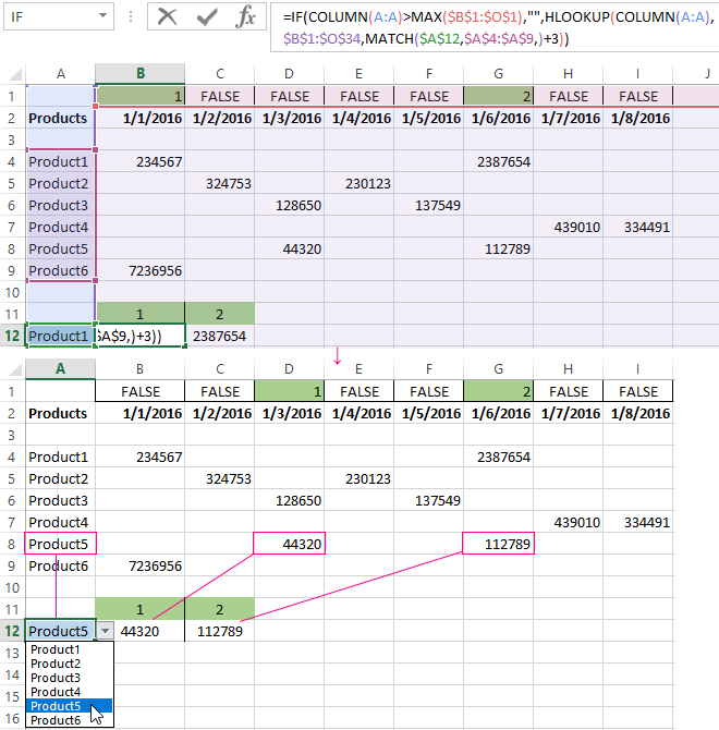
Download examples of advanced filtering

Thus, using the tool «Drop-down list» and built-in functions Excel selects data in rows according to a certain criterion.

Источник

Examples

Need more help?

See Also

Need more help?

Filter a range of data

Filter data in a table

Related Topics

Filter data in a table

Filter a range of data

Filtering options for tables or ranges

To clear a filter from a column

To remove all the filters from a table or range

Need more help?

What is Filter in Excel?

Table of contents

How to Filter in Excel?

Method 1: With Filter Option Under the Home tab

Method 2: With Filter Option Under the Data tab

Method 3: With the Shortcut key

How to Add Filters in Excel?

Example #1–“Number Filters” Option

Example #2–“Search Box” Option

Option while you Drop Down the Filter Function

The Techniques of Filtering in Excel

Frequently Asked Questions

Recommended Articles

Here are the Excel Filters formulas:

Filter by a number

Filter by a cell value

Filter by a text string

Filter where NOT equal to

Filter by date

Filter by multiple conditions

Filter from another sheet

Excel description for FILTER function:

Filtering by a single condition in Excel

Part 1: How to filter by a number

Operators that can be used in the FILTER function:

Part 2: How to filter by a cell value in Excel

Part 3: How to filter by text in Excel

Part 4: Using NOT EQUAL TO in the Excel FILTER function

Part 4: How to filter by date in Excel

Filter by date in Excel example 1:

Filter by date in Excel example 2:

Filter by multiple conditions in Excel

Part 5: Filtering by 2 conditions where BOTH MUST BE TRUE

Part 6: Filtering by 2 conditions where EITHER ARE TRUE, not necessarily both

How to filter from another sheet in Excel

Pop Quiz: Test your knowledge

Question #1

Question #2

Question #3

Question #4

Question #5

Answers to the questions above:

How to make the advanced filter in Excel?

How to use the advanced filter in Excel?

How to make few filters in Excel?

How to make the filter in Excel by lines?