
If the data you want to filter requires complex criteria (such as Type = «Produce» OR Salesperson = «Davolio»), you can use the Advanced Filter dialog box.
To open the Advanced Filter dialog box, click Data > Advanced.

|
Advanced Filter |
Example |
|---|---|
|
Overview of advanced filter criteria |
|
|
Multiple criteria, one column, any criteria true |
Salesperson = «Davolio» OR Salesperson = «Buchanan» |
|
Multiple criteria, multiple columns, all criteria true |
Type = «Produce» AND Sales > 1000 |
|
Multiple criteria, multiple columns, any criteria true |
Type = «Produce» OR Salesperson = «Buchanan» |
|
Multiple sets of criteria, one column in all sets |
(Sales > 6000 AND Sales < 6500 ) OR (Sales < 500) |
|
Multiple sets of criteria, multiple columns in each set |
(Salesperson = «Davolio» AND Sales >3000) OR |
|
Wildcard criteria |
Salesperson = a name with ‘u’ as the second letter |
Overview of advanced filter criteria
The Advanced command works differently from the Filter command in several important ways.
-
It displays the Advanced Filter dialog box instead of the AutoFilter menu.
-
You type the advanced criteria in a separate criteria range on the worksheet and above the range of cells or table that you want to filter. Microsoft Office Excel uses the separate criteria range in the Advanced Filter dialog box as the source for the advanced criteria.
Sample data
The following sample data is used for all procedures in this article.
The data includes four blank rows above the list range that will be used as a criteria range (A1:C4) and a list range (A6:C10). The criteria range has column labels and includes at least one blank row between the criteria values and the list range.
To work with this data, select it in the following table, copy it, and then paste it in cell A1 of a new Excel worksheet.
|
Type |
Salesperson |
Sales |
|
Type |
Salesperson |
Sales |
|
Beverages |
Suyama |
$5122 |
|
Meat |
Davolio |
$450 |
|
produce |
Buchanan |
$6328 |
|
Produce |
Davolio |
$6544 |
Comparison operators
You can compare two values by using the following operators. When two values are compared by using these operators, the result is a logical value—either TRUE or FALSE.
|
Comparison operator |
Meaning |
Example |
|---|---|---|
|
= (equal sign) |
Equal to |
A1=B1 |
|
> (greater than sign) |
Greater than |
A1>B1 |
|
< (less than sign) |
Less than |
A1<B1 |
|
>= (greater than or equal to sign) |
Greater than or equal to |
A1>=B1 |
|
<= (less than or equal to sign) |
Less than or equal to |
A1<=B1 |
|
<> (not equal to sign) |
Not equal to |
A1<>B1 |
Using the equal sign to type text or a value
Because the equal sign (=) is used to indicate a formula when you type text or a value in a cell, Excel evaluates what you type; however, this may cause unexpected filter results. To indicate an equality comparison operator for either text or a value, type the criteria as a string expression in the appropriate cell in the criteria range:
=»=
entry
»
Where entry is the text or value you want to find. For example:
|
What you type in the cell |
What Excel evaluates and displays |
|---|---|
|
=»=Davolio» |
=Davolio |
|
=»=3000″ |
=3000 |
Considering case-sensitivity
When filtering text data, Excel doesn’t distinguish between uppercase and lowercase characters. However, you can use a formula to perform a case-sensitive search. For an example, see the section Wildcard criteria.
Using pre-defined names
You can name a range Criteria, and the reference for the range will appear automatically in the Criteria range box. You can also define the name Database for the list range to be filtered and define the name Extract for the area where you want to paste the rows, and these ranges will appear automatically in the List range and Copy to boxes, respectively.
Creating criteria by using a formula
You can use a calculated value that is the result of a formula as your criterion. Remember the following important points:
-
The formula must evaluate to TRUE or FALSE.
-
Because you are using a formula, enter the formula as you normally would, and do not type the expression in the following way:
=»=
entry
» -
Do not use a column label for criteria labels; either keep the criteria labels blank or use a label that is not a column label in the list range (in the examples that follow, Calculated Average and Exact Match).
If you use a column label in the formula instead of a relative cell reference or a range name, Excel displays an error value such as #NAME? or #VALUE! in the cell that contains the criterion. You can ignore this error because it does not affect how the list range is filtered.
-
The formula that you use for criteria must use a relative reference to refer to the corresponding cell in the first row of data.
-
All other references in the formula must be absolute references.
Multiple criteria, one column, any criteria true
Boolean logic: (Salesperson = «Davolio» OR Salesperson = «Buchanan»)
-
Insert at least three blank rows above the list range that can be used as a criteria range. The criteria range must have column labels. Make sure that there is at least one blank row between the criteria values and the list range.
-
To find rows that meet multiple criteria for one column, type the criteria directly below each other in separate rows of the criteria range. Using the example, enter:
Type
Salesperson
Sales
=»=Davolio»
=»=Buchanan»
-
Click a cell in the list range. Using the example, click any cell in the range A6:C10.
-
On the Data tab, in the Sort & Filter group, click Advanced.

-
Do one of the following:
-
To filter the list range by hiding rows that don’t match your criteria, click Filter the list, in-place.
-
To filter the list range by copying rows that match your criteria to another area of the worksheet, click Copy to another location, click in the Copy to box, and then click the upper-left corner of the area where you want to paste the rows.
Tip When you copy filtered rows to another location, you can specify which columns to include in the copy operation. Before filtering, copy the column labels for the columns that you want to the first row of the area where you plan to paste the filtered rows. When you filter, enter a reference to the copied column labels in the Copy to box. The copied rows will then include only the columns for which you copied the labels.
-
-
In the Criteria range box, enter the reference for the criteria range, including the criteria labels. Using the example, enter $A$1:$C$3.
To move the Advanced Filter dialog box out of the way temporarily while you select the criteria range, click Collapse Dialog
. -
Using the example, the filtered result for the list range is:
Type
Salesperson
Sales
Meat
Davolio
$450
produce
Buchanan
$6,328
Produce
Davolio
$6,544
 .
.Multiple criteria, multiple columns, all criteria true
Boolean logic: (Type = «Produce» AND Sales > 1000)
-
Insert at least three blank rows above the list range that can be used as a criteria range. The criteria range must have column labels. Make sure that there is at least one blank row between the criteria values and the list range.
-
To find rows that meet multiple criteria in multiple columns, type all the criteria in the same row of the criteria range. Using the example, enter:
Type
Salesperson
Sales
=»=Produce»
>1000
-
Click a cell in the list range. Using the example, click any cell in the range A6:C10.
-
On the Data tab, in the Sort & Filter group, click Advanced.
-
Do one of the following:
-
To filter the list range by hiding rows that don’t match your criteria, click Filter the list, in-place.
-
To filter the list range by copying rows that match your criteria to another area of the worksheet, click Copy to another location, click in the Copy to box, and then click the upper-left corner of the area where you want to paste the rows.
Tip When you copy filtered rows to another location, you can specify which columns to include in the copy operation. Before filtering, copy the column labels for the columns that you want to the first row of the area where you plan to paste the filtered rows. When you filter, enter a reference to the copied column labels in the Copy to box. The copied rows will then include only the columns for which you copied the labels.
-
-
In the Criteria range box, enter the reference for the criteria range, including the criteria labels. Using the example, enter $A$1:$C$2.
To move the Advanced Filter dialog box out of the way temporarily while you select the criteria range, click Collapse Dialog
. -
Using the example, the filtered result for the list range is:
Type
Salesperson
Sales
produce
Buchanan
$6,328
Produce
Davolio
$6,544
Multiple criteria, multiple columns, any criteria true
Boolean logic: (Type = «Produce» OR Salesperson = «Buchanan»)
-
Insert at least three blank rows above the list range that can be used as a criteria range. The criteria range must have column labels. Make sure that there is at least one blank row between the criteria values and the list range.
-
To find rows that meet multiple criteria in multiple columns where any criteria can be true, type the criteria in the different columns and rows of the criteria range. Using the example, enter:
Type
Salesperson
Sales
=»=Produce»
=»=Buchanan»
-
Click a cell in the list range. Using the example, click any cell in the list range A6:C10.
-
On the Data tab, in the Sort & Filter group, click Advanced.
-
Do one of the following:
-
To filter the list range by hiding rows that don’t match your criteria, click Filter the list, in-place.
-
To filter the list range by copying rows that match your criteria to another area of the worksheet, click Copy to another location, click in the Copy to box, and then click the upper-left corner of the area where you want to paste the rows.
Tip: When you copy filtered rows to another location, you can specify which columns to include in the copy operation. Before filtering, copy the column labels for the columns that you want to the first row of the area where you plan to paste the filtered rows. When you filter, enter a reference to the copied column labels in the Copy to box. The copied rows will then include only the columns for which you copied the labels.
-
-
In the Criteria range box, enter the reference for the criteria range, including the criteria labels. Using the example, enter $A$1:$B$3.
To move the Advanced Filter dialog box out of the way temporarily while you select the criteria range, click Collapse Dialog
. -
Using the example, the filtered result for the list range is:
Type
Salesperson
Sales
produce
Buchanan
$6,328
Produce
Davolio
$6,544
Multiple sets of criteria, one column in all sets
Boolean logic: ( (Sales > 6000 AND Sales < 6500 ) OR (Sales < 500) )
-
Insert at least three blank rows above the list range that can be used as a criteria range. The criteria range must have column labels. Make sure that there is at least one blank row between the criteria values and the list range.
-
To find rows that meet multiple sets of criteria where each set includes criteria for one column, include multiple columns with the same column heading. Using the example, enter:
Type
Salesperson
Sales
Sales
>6000
<6500
<500
-
Click a cell in the list range. Using the example, click any cell in the list range A6:C10.
-
On the Data tab, in the Sort & Filter group, click Advanced.
-
Do one of the following:
-
To filter the list range by hiding rows that don’t match your criteria, click Filter the list, in-place.
-
To filter the list range by copying rows that match your criteria to another area of the worksheet, click Copy to another location, click in the Copy to box, and then click the upper-left corner of the area where you want to paste the rows.
Tip: When you copy filtered rows to another location, you can specify which columns to include in the copy operation. Before filtering, copy the column labels for the columns that you want to the first row of the area where you plan to paste the filtered rows. When you filter, enter a reference to the copied column labels in the Copy to box. The copied rows will then include only the columns for which you copied the labels.
-
-
In the Criteria range box, enter the reference for the criteria range, including the criteria labels. Using the example, enter $A$1:$D$3.
To move the Advanced Filter dialog box out of the way temporarily while you select the criteria range, click Collapse Dialog
. -
Using the example, the filtered result for the list range is:
Type
Salesperson
Sales
Meat
Davolio
$450
produce
Buchanan
$6,328
Multiple sets of criteria, multiple columns in each set
Boolean logic: ( (Salesperson = «Davolio» AND Sales >3000) OR (Salesperson = «Buchanan» AND Sales > 1500) )
-
Insert at least three blank rows above the list range that can be used as a criteria range. The criteria range must have column labels. Make sure that there is at least one blank row between the criteria values and the list range.
-
To find rows that meet multiple sets of criteria, where each set includes criteria for multiple columns, type each set of criteria in separate columns and rows. Using the example, enter:
Type
Salesperson
Sales
=»=Davolio»
>3000
=»=Buchanan»
>1500
-
Click a cell in the list range. Using the example, click any cell in the list range A6:C10.
-
On the Data tab, in the Sort & Filter group, click Advanced.
-
Do one of the following:
-
To filter the list range by hiding rows that don’t match your criteria, click Filter the list, in-place.
-
To filter the list range by copying rows that match your criteria to another area of the worksheet, click Copy to another location, click in the Copy to box, and then click the upper-left corner of the area where you want to paste the rows.
Tip When you copy filtered rows to another location, you can specify which columns to include in the copy operation. Before filtering, copy the column labels for the columns that you want to the first row of the area where you plan to paste the filtered rows. When you filter, enter a reference to the copied column labels in the Copy to box. The copied rows will then include only the columns for which you copied the labels.
-
-
In the Criteria range box, enter the reference for the criteria range, including the criteria labels. Using the example, enter $A$1:$C$3.To move the Advanced Filter dialog box out of the way temporarily while you select the criteria range, click Collapse Dialog
. -
Using the example, the filtered result for the list range would be:
Type
Salesperson
Sales
produce
Buchanan
$6,328
Produce
Davolio
$6,544
Wildcard criteria
Boolean logic: Salesperson = a name with ‘u’ as the second letter
-
To find text values that share some characters but not others, do one or more of the following:
-
Type one or more characters without an equal sign (=) to find rows with a text value in a column that begin with those characters. For example, if you type the text Dav as a criterion, Excel finds «Davolio,» «David,» and «Davis.»
-
Use a wildcard character.
Use
To find
? (question mark)
Any single character
For example, sm?th finds «smith» and «smyth»* (asterisk)
Any number of characters
For example, *east finds «Northeast» and «Southeast»~ (tilde) followed by ?, *, or ~
A question mark, asterisk, or tilde
For example, fy91~? finds «fy91?»
-
-
Insert at least three blank rows above the list range that can be used as a criteria range. The criteria range must have column labels. Make sure that there is at least one blank row between the criteria values and the list range.
-
In the rows below the column labels, type the criteria that you want to match. Using the example, enter:
Type
Salesperson
Sales
=»=Me*»
=»=?u*»
-
Click a cell in the list range. Using the example, click any cell in the list range A6:C10.
-
On the Data tab, in the Sort & Filter group, click Advanced.
-
Do one of the following:
-
To filter the list range by hiding rows that don’t match your criteria, click Filter the list, in-place
-
To filter the list range by copying rows that match your criteria to another area of the worksheet, click Copy to another location, click in the Copy to box, and then click the upper-left corner of the area where you want to paste the rows.
Tip: When you copy filtered rows to another location, you can specify which columns to include in the copy operation. Before filtering, copy the column labels for the columns that you want to the first row of the area where you plan to paste the filtered rows. When you filter, enter a reference to the copied column labels in the Copy to box. The copied rows will then include only the columns for which you copied the labels.
-
-
In the Criteria range box, enter the reference for the criteria range, including the criteria labels. Using the example, enter $A$1:$B$3.
To move the Advanced Filter dialog box out of the way temporarily while you select the criteria range, click Collapse Dialog
. -
Using the example, the filtered result for the list range is:
Type
Salesperson
Sales
Beverages
Suyama
$5,122
Meat
Davolio
$450
produce
Buchanan
$6,328
Need more help?
You can always ask an expert in the Excel Tech Community or get support in the Answers community.
Watch Video – Excel Advanced Filter
Excel Advanced Filter is one of the most underrated and under-utilized features that I have come across.
If you work with Excel, I am sure you have used (or at least heard about the regular excel filter). It quickly filters a data set based on selection, specified text, number or other such criteria.
In this guide, I will show you some cool stuff you can do using the Excel advanced filter.
But First… What is Excel Advanced Filter?
Excel Advanced Filter – as the name suggests – is the advanced version of the regular filter. You can use this when you need to use more complex criteria to filter your data set.
Here are some differences between the regular filter and Advanced filter:
- While the regular data filter will filter the existing dataset, you can use Excel advanced filter to extract the data set to some other location as well.
- Excel Advanced Filter allows you to use complex criteria. For example, if you have sales data, you can filter data on a criterion where the sales rep is Bob and the region is either North or South (we will see how to do this in examples). Office support has some good explanation on this.
- You can use the Excel Advanced Filter to extract unique records from your data (more on this in a second).
EXCEL ADVANCED FILTER (Examples)
Now let’s have a look at some example on using the Advanced Filter in Excel.
Example 1 – Extracting a Unique list
You can use Excel Advanced Filter to quickly extract unique records from a data set (or in other words remove duplicates).
In Excel 2007 and later versions, there is an option to remove duplicates from a dataset. But that alters your existing data set. To keep the original data intact, you need to create a copy of the data and then use the Remove Duplicates option. Excel Advanced filter would allow you to select a location to get a unique list.
Let’s see how to use an advanced filters to get a unique list.
Suppose you have a dataset as shown below:
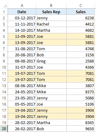
As you can see, there are duplicate records in this data set (highlighted in orange). These could be due to an error in data entry or result of data compilation.
In such a case, you can use Excel Advanced Filter tool to quickly get a list of all the unique records in a different location (so that your original data remains intact).
Here are the steps to get all the unique records:
This will instantly give you a list of all the unique records.

Caution: When you are using Advanced Filter to get the unique list, make sure you have also selected the header. If you don’t, it would consider the first cell as the header.
Example 2 – Using Criteria in Excel Advanced Filter
Getting unique records is one of the many things you can do with Excel advanced filter.
Its primary utility lies in its ability to allow using complex criteria for filtering data.
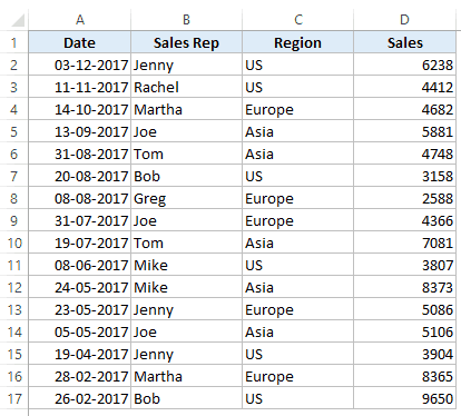
Here is what I mean by complex criteria. Suppose you have a dataset as shown below and you want to quickly get all the records where the sales are greater than 5000 and the region is the US.
Here is how you can use Excel Advanced Filter to filter the records based on the specified criteria:
This would instantly give you all the records where the region is the US and the sales are more than 5000.

The above example is a case where the filtering is done based on two criteria (US and sales greater than 5000).
Excel Advanced filter allows you to create many different combinations of criteria.
Here are some examples of how you can construct these filters.
Using the AND Criteria
When you want to use AND criteria, you need to specify it below the header.
For example:
Using the OR Criteria
When you want to use OR criteria, you need to specify the criteria in the same column.
For example:
By now, you must have realized that when we have the criteria in the same row, it is an AND criteria, and when we have it in different rows, it is an OR criteria.
Example 3 – Using WILDCARD Characters in Advanced Filter in Excel
Excel Advanced Filter also allows the usage of wildcard characters while constructing the criteria.
There are three wildcard characters in Excel:
- * (asterisk) – It represents any number of characters. For example, ex* could mean excel, excels, example, expert, etc.
- ? (question mark) – It represents one single character. For example, Tr?mp could mean Trump or Tramp.
- ~ (tilde) – It is used to identify a wildcard character (~, *, ?) in the text.
Now let’s see how we can use these wildcard characters to do some advanced filtering in Excel.
- To filter records where the sales rep name starts from J.

Note that * represent any number of characters. So any rep with the name starting with J would be filtered with these criteria.
Similarly, you can use the other two wildcard characters as well.
Note: In case you’re using Office 365, you should check out the FILTER function. It can do a lot of things that advanced filter can do with a simple formula.
NOTE:
- Remember, the headers in the criteria should be exactly the same as that in the data set.
- Advanced filtering cannot be undone when copied to other locations.
You May Also Like the Following Excel Tutorials:
- Dynamic Excel Filter – Extract Data as you Type.
- Filtering Cells with Bold Font Formatting.
- How to Filter Cells that have Duplicate Text Strings (Words) in it.
- How to Filter Data in a Pivot Table in Excel
- MS Guide for Advanced Filter in Excel.
- How to Compare Two Columns in Excel.
- Excel VBA Autofilter
- 20 Advanced Excel Functions and Formulas (for Excel Pros)
Advanced filter in Excel provides more opportunities for managing on data management spreadsheets. It is more complex in settings, but much more effective in action.
Using a standard filter, a Microsoft Excel user can solve not all of the tasks that are set. There is no visual display of the applied filtering conditions. It is not possible to apply more than two selection criteria. You can not filter the duplicate values to leave only unique records. And the criteria themselves are schematic and simple. The functionality of the extended filter is much richer. Let’s take a closer look at its possibilities.
How to make the advanced filter in Excel?
The advanced filter allows you to analysis data on an unlimited set of conditions. With this tool, the user can:
- to specify more than two selection criteria;
- to copy the result of filtering to another sheet;
- to set the condition of any complexity with the helping of formulas;
- to extract the unique values.
The algorithm for applying the extended filter is simple.
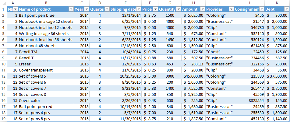
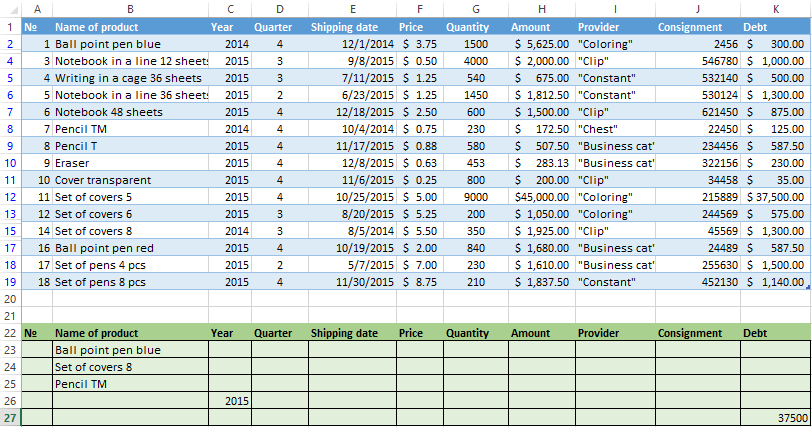
- To make the table with the original data or to open an existing one. Like so:
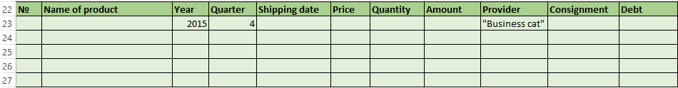
- To create the condition table. The features: the header line is the same with the «cap» of the filtered table. To avoid errors, need to copy the header line in the source table and paste it on the same sheet (side, top, underarm) or on another sheet. We enter the selection criteria into the condition table.
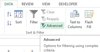
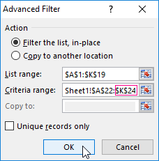
- Go to the «DATA» tab — «Sort and filter» — «Advanced». If the filtered information should be displayed on another sheet (NOT where the source table is), then you need to run the extended filter from another sheet.
- In the «Advanced Filter» window that opens, to select the method of processing information (on the same sheet or on the other one), set the initial range (the table 1, example) and the range of conditions (the table 2, conditions). The header lines must be included in the ranges.
- To close the «Advanced Filter» window, click OK. We see the result.
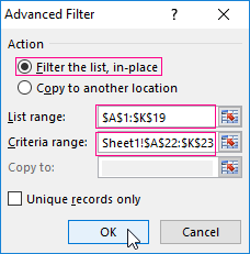

The top table is the result of the filtering. The lower nameplate with the conditions is given for clarity near.
How to use the advanced filter in Excel?
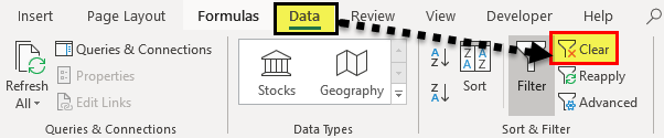
To cancel the action of the advanced filter, we place the cursor anywhere in the table and press Ctrl + Shift + L or «DATA» — «Sort and Filter» — «Clear».
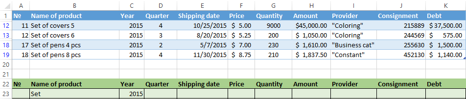
We will find using the «Advanced Filter» tool information on the values that contain the word «Set».
In the table of conditions we bring in the criteria. For example, these are:

The program in this case will search for all information on the goods, in the title of which there is the word «Set».
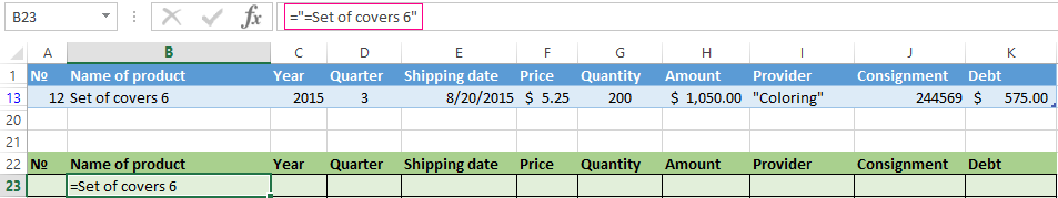
To search for the exact value, you can use the «=» sign. We enter the following criteria in the condition table:

Excel sees the «=» as a signal: the user will set the formula now. In order for the program to work correctly, the following should be written in the formula line: =»=Set of covers 6″.
After using the «Advanced Filter»:
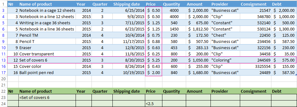
We filter the source table by the condition «OR» for different columns now. The operator «OR» is also in the tool «AutoFilter». But there it can be used within the single column.
In the condition label we introduce the selection criteria: =»=Set of covers 6″. (In the column «Name of product») and = «<2.5$» (in the column «Price»). That is, the program must select those values that contain the EXACTLY information about the good «Set of covers 6 ». OR to the information about the goods, which price is <2.5.

Please note: the criteria must be written under the corresponding headings in the DIFFERENT lines.
The result of selection:
The advanced filter allows you to use as a criterion of a formula. Let’s consider the example.

Selection of the line with the maximum indebtedness: =MAX(Table1[Debt]).
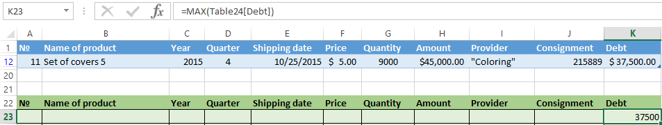
So we get the results as after running several filters on the one Excel sheet.
How to make few filters in Excel?
Let’s create the filter by several values. To do this, we enter in the table of conditions several criteria for selecting data:
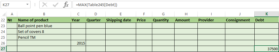
Apply the tool «Advanced Filter»:
Now from the table with the selected data we will extract new information, which was selected according to other criteria. There are only shipping date for autumn 2015 (from September to November). Example:
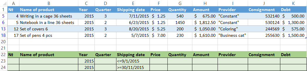
We introduce a new criterion in the condition table and apply the filtering tool. The initial range — is the table with data selected according to the previous criterion. This is how the filter is performed across on several columns.
To use few filters, you can create several condition tables on the new sheets. The method of implementation depends from the task which was set by user.
How to make the filter in Excel by lines?
By standard methods — you may not do it by any ways. Microsoft Excel selects data only in columns. Therefore, we need to look for other solutions.
Here are some examples of string criteria for the extended filter in Excel:
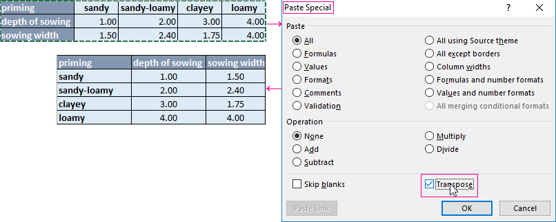
- Convert to the table. For example, from three rows make a list of three columns and apply the filtering to the transformed version.
- Use formulas to display exactly the data in the string that are needed. For example, make some indicator drop-down list. And in the next cell, enter the formula using the IF function. When a certain value is selected from the drop-down list, its parameter appears next to it.
To give an example of how the filter works by rows in Excel, we are creating the label:
For the list of products, we create the drop-down list:
If necessary, learn how to create a drop-down list in Excel.
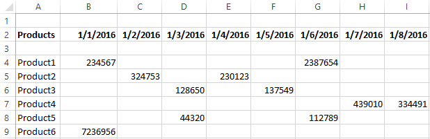
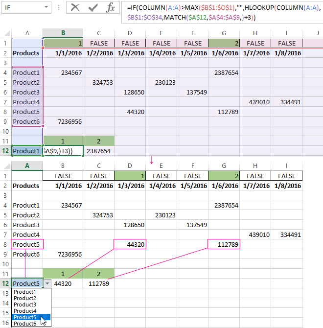
Above the table with the original data, we insert an empty line. In the cells, we introduce the formula that will show which columns the information is taken from.
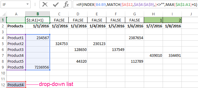
Next to the drop-down list box, we enter the following formula:
Its task is select from the table those values, that correspond to a certain good.
Download examples of advanced filtering
Thus, using the tool «Drop-down list» and built-in functions Excel selects data in rows according to a certain criterion.
The advanced filter is different from the auto filter in Excel. This feature is not like a button that one can use with a single click of the mouse. To use an advanced filter, we have to define criteria for the auto filter and then click on the “Data” tab. Then, in the advanced section for the advanced filter, we will fill our criteria for the data.
For example, suppose you have a dataset. In this dataset, there are duplicate records. That could be due to an error in the data entry or a data compilation. We can use Excel Advanced Filter Tool to receive unique records in other locations, retaining the original data.
Table of contents
- What is Advanced Filter in Excel?
- How to Use Advanced Filter in Excel? (With Examples)
- Example #1
- Example #2
- Example #3
- Example #4
- Example #5
- Example #6 – Using WILDCARD Characters
- Example #7
- Things to Remember
- Recommended Articles
- How to Use Advanced Filter in Excel? (With Examples)
How to Use Advanced Filter in Excel? (With Examples)
Let us learn the use of this with some examples.
You can download this Advanced Filter Excel Template here – Advanced Filter Excel Template
Example #1
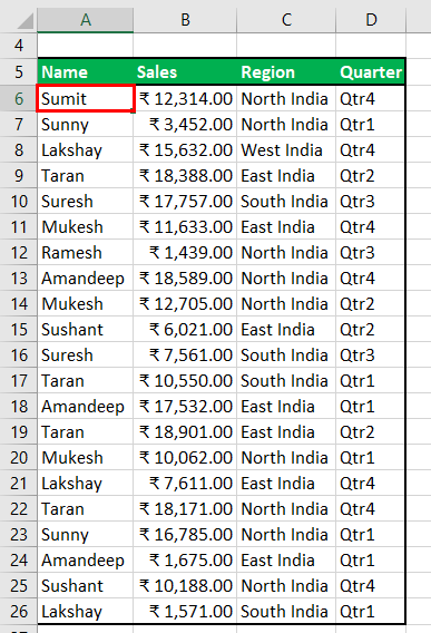
Suppose we have the following data to filter based on different criteria:
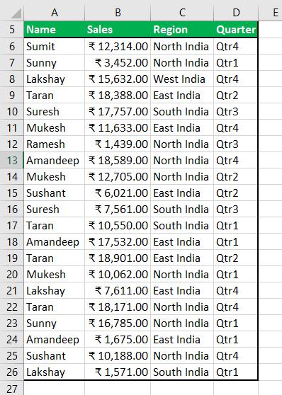
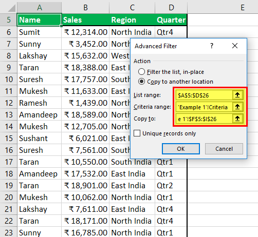
We need to check the sales transaction made by “Taran” and “Suresh.” Then, we can use the OR operator, displaying the records satisfying any conditions. Then, we can follow the steps to apply these filters in Excel to get the results.
Below are the steps for applying an advanced filter in Excel: –
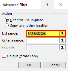
- To use an advanced filter, first, we need to select any of the cells in the data range.

- Click on the “Data tab” – “Sort & Filter” group – “Advanced” command.

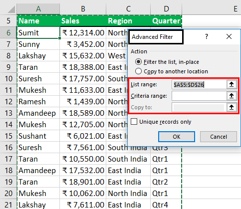
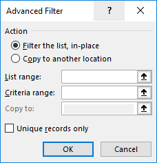
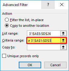
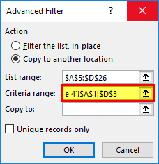
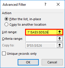
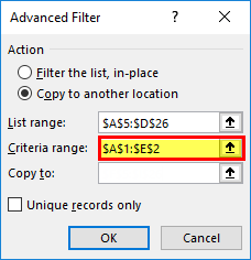
- As we click on “Advanced,” a dialog box “Advanced Filter” will open for asking “List Range” to filter, “Criteria Range” for defining the criteria, and “Extract Range” for copying the filtered data (if desired).

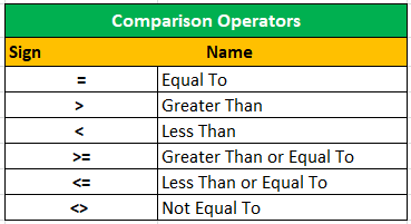
- For “Criteria Range,” we need to copy the column headings on the top row and define the criteria below the field heading. To specify the criteria, we can use the comparison operator, which is as follows:


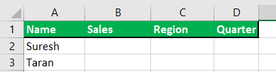
- We want to get all records having the name ‘Suresh’ or ‘Taran.’ The Criteria Range would be like below:

For “OR” conditions where we want to display the records that satisfy any requirement, we must specify the criteria in different rows.
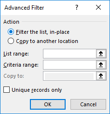
There are two actions in an advanced filter.
- Filter the list in place: This option filters the list at the original position, i.e., on the “List Range.”After analyzing, we can remove the filter using the “Clear” command in the “Sort & Filter” group under “Data.”
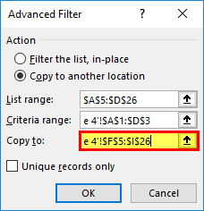
- Copy to another location: This option copies the desired data according to the criteria to the specified range.
We can use any option according to our needs, but we will use the 2nd option more often.
Now, we need to:
- First, open the “Advanced Filter” dialog box.
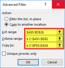
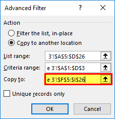
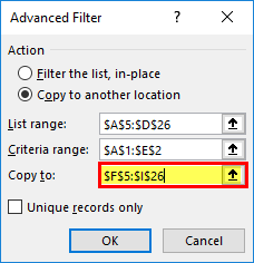
- Specifying the “List Range” as $A$5:$D$26, “Criteria Range” as $A$1:$D$3, and “Copy to” Range as $F$5:$I$26. Click on “OK.
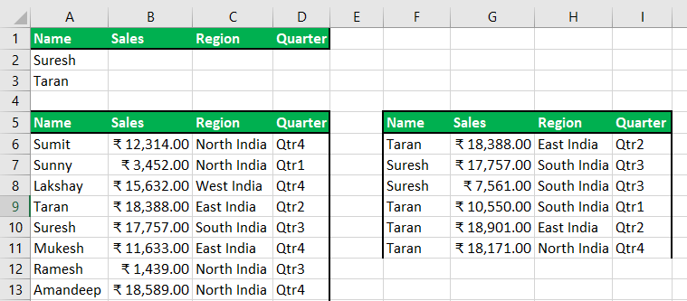
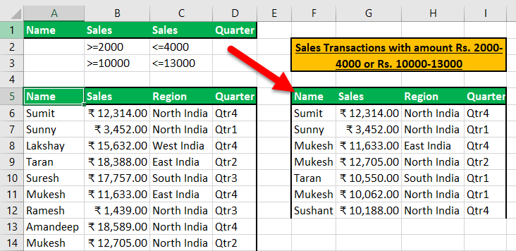
All the records with names ‘Suresh’ or ‘Taran’ are filtered out and displayed separately in a different cell range.
Example #2
We want all the sales transactions of Qtr 1 and South India. Therefore, the “Criteria Range” is as below:
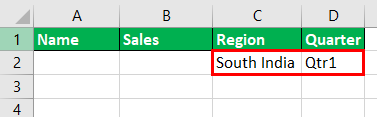
As we have the ‘AND’ condition here, we want to display the records where both conditions are met. Therefore, we have mentioned the criteria below both column headings in the same row.
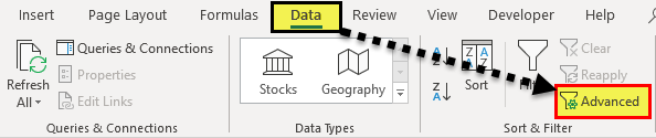
Now, we will click on the “Advanced” command in the “Sort & Filter” group under the “Data” tab.
From the ‘Advanced Filter” dialog box, we will choose “Copy to another location” and then define the A5: D26 as List Range, A1: D2 as “Criteria Range,” and F5:I26 as “Copy To” range.
Now the result is as follows:

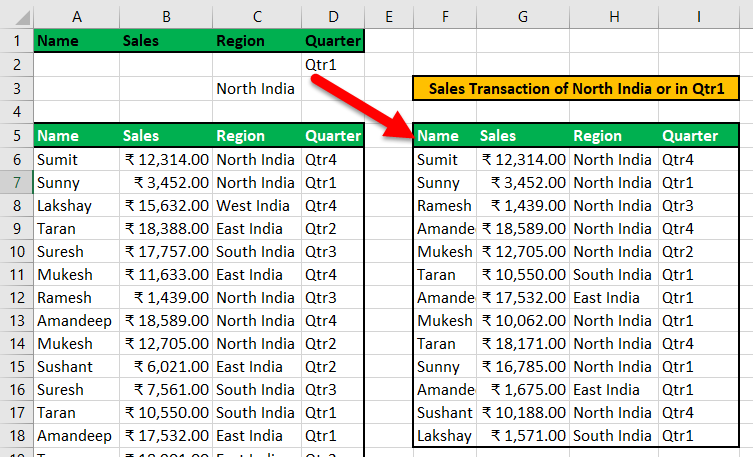
Example #3
We want to find sales in Qtr 1 or made in North India.
We need to specify both the criteria in different rows and different columns. We have to display the data if any conditions are met, and both are related to different columns.
Steps:
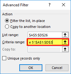
- We need to open the “Advanced Filter” dialog box.
- We will specify “List Range” as $A$5:$D$26.

- Also, specify “Criteria Range” as $A$1:$D$3.
- And, specify the “Copy To” range as $F$5:$I$26.
The result would be as follows:
Example #4
Now, we want to find all sales of ₹2,000 – ₹4,000 and ₹10,000 – ₹13,000.

As we have four conditions,
(Condition 1 AND Condition 2) OR (Condition 3 AND Condition 4).
(>=2000 AND <=4000) OR (>=10000 AND <=13000)
We have mentioned the conditions with “AND” in the same row and “OR” in different rows.
Steps:
- To open the “Advanced Filter” dialog box, we will click on “Advanced” in the “Sort & Filter” group under “Data.”
- In the “Advanced Filter” dialog box, we will specify “List Range” as $A$5:$D$26
- And, we will specify the “Criteria Range” as $A$1:$D$3
- Also, “Copy to” Range as $F$5:$I$26
- After clicking on “OK,“ the result will be:
Example #5
We want to find the sales of Qtr 1 by Sunny or that of Qtr 3 by Mukesh.

As we have AND and OR, both relations in conditions, we will specify the conditions in the criteria range in different rows (OR) and other columns (AND).
Steps:
- To open the “Advanced Filter” dialog box, we will click on “Advanced” in the “Sort & Filter” group under “Data.“
- In the “Advanced Filter” dialog box, we specify “List Range” as $A$5:$D$26.

- And we will specify the “Criteria Range” as $A$1:$D$3.
- Also, “Copy to” Range as $F$5:$I$26.

- After clicking on “OK”, then the result would be:

Example #6 – Using WILDCARD Characters
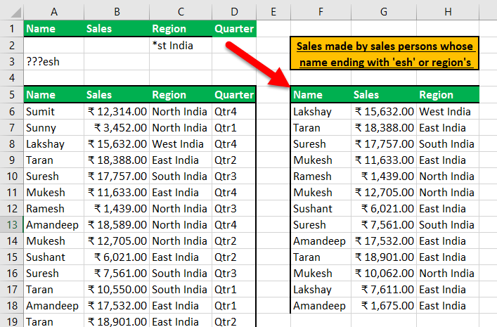
We want to find all the sales transactions with a name ending with “esh” or a region’s first word ending with “st” and only want to retrieve the name, sales, and region.
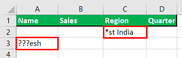
Here, * denotes more than one character, and “?” represents only one character.
Before implementing the advanced filter, we need to specify the column labels on “Copy to Range” as we want only some columns, not all.

Now, we will call the command.
Steps:
- To open the ‘Advanced Filter’ dialog box, we will click on ‘Advanced’ in the ‘Sort & Filter’ group under ‘Data.’
- In the “Advanced Filter” dialog box, we specify “List Range” as $A$5:$D$26.
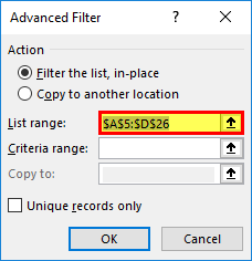
- We will specify the “Criteria Range” as $A$1:$D$3
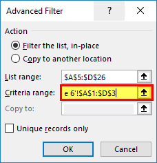
- Also, “Copy to” Range as $F$5:$H$26

- After clicking on “OK,” then the result would be:
Example #7
We want to filter the top five sales (of a large amount).

The formula cell must evaluate TRUE or FALSE to get the most significant five records. Hence, we used the LARGE Excel function and compared the value with the sales amount.
As we can see, the column heading for the formula cell is blank. Therefore, we can either keep it empty or give it a name that does not match the column headings in the data range.
We will specify the ranges in the “Advanced Filter” dialog box. Steps are:
- To open the “Advanced Filter” dialog box, we will click on “Advanced” in the “Sort & Filter” group under “Data.”
- In the “Excel Advanced Filter” dialog box, we will specify “List Range” as $A$5:$D$26.
- And “Criteria Range” as $A$1:$E$2
- Also,“Copy to” Range as $F$5:$I$26
- After clicking on “OK,” then, the result would be like this:

Things to Remember
- The range it needs to be applied must have a unique heading, as duplicate headers cause problems when running an advanced filter.
- There should be at least one blank row between the “List Range” and “Criteria Range.”
Recommended Articles
This article is a guide to Advanced Filter in Excel. We discussed using Advanced Filter in Excel, along with Excel examples and downloadable excel templates. You may also look at these useful Excel tools: –
- Add Filter in Excel
- Filter Shortcut in Excel
- Auto Filter In Excel
- Sort Data in Excel
- Compound Interest Formula in Excel
Расширенный фильтр и немного магии
У подавляющего большинства пользователей Excel при слове «фильтрация данных» в голове всплывает только обычный классический фильтр с вкладки Данные — Фильтр (Data — Filter):

Такой фильтр — штука привычная, спору нет, и для большинства случаев вполне сойдет. Однако бывают ситуации, когда нужно проводить отбор по большому количеству сложных условий сразу по нескольким столбцам. Обычный фильтр тут не очень удобен и хочется чего-то помощнее. Таким инструментом может стать расширенный фильтр (advanced filter), особенно с небольшой «доработкой напильником» (по традиции).
Основа
Для начала вставьте над вашей таблицей с данными несколько пустых строк и скопируйте туда шапку таблицы — это будет диапазон с условиями (выделен для наглядности желтым):

Между желтыми ячейками и исходной таблицей обязательно должна быть хотя бы одна пустая строка.
Именно в желтые ячейки нужно ввести критерии (условия), по которым потом будет произведена фильтрация. Например, если нужно отобрать бананы в московский «Ашан» в III квартале, то условия будут выглядеть так:

Чтобы выполнить фильтрацию выделите любую ячейку диапазона с исходными данными, откройте вкладку Данные и нажмите кнопку Дополнительно (Data — Advanced). В открывшемся окне должен быть уже автоматически введен диапазон с данными и нам останется только указать диапазон условий, т.е. A1:I2:

Обратите внимание, что диапазон условий нельзя выделять «с запасом», т.е. нельзя выделять лишние пустые желтые строки, т.к. пустая ячейка в диапазоне условий воспринимается Excel как отсутствие критерия, а целая пустая строка — как просьба вывести все данные без разбора.
Переключатель Скопировать результат в другое место позволит фильтровать список не прямо тут же, на этом листе (как обычным фильтром), а выгрузить отобранные строки в другой диапазон, который тогда нужно будет указать в поле Поместить результат в диапазон. В данном случае мы эту функцию не используем, оставляем Фильтровать список на месте и жмем ОК. Отобранные строки отобразятся на листе:

Добавляем макрос
«Ну и где же тут удобство?» — спросите вы и будете правы. Мало того, что нужно руками вводить условия в желтые ячейки, так еще и открывать диалоговое окно, вводить туда диапазоны, жать ОК. Грустно, согласен! Но «все меняется, когда приходят они ©» — макросы!
Работу с расширенным фильтром можно в разы ускорить и упростить с помощью простого макроса, который будет автоматически запускать расширенный фильтр при вводе условий, т.е. изменении любой желтой ячейки. Щелкните правой кнопкой мыши по ярлычку текущего листа и выберите команду Исходный текст (Source Code). В открывшееся окно скопируйте и вставьте вот такой код:
Private Sub Worksheet_Change(ByVal Target As Range)
    If Not Intersect(Target, Range("A2:I5")) Is Nothing Then
        On Error Resume Next
        ActiveSheet.ShowAllData
        Range("A7").CurrentRegion.AdvancedFilter Action:=xlFilterInPlace, CriteriaRange:=Range("A1").CurrentRegion
    End If
End Sub
Эта процедура будет автоматически запускаться при изменении любой ячейки на текущем листе. Если адрес измененной ячейки попадает в желтый диапазон (A2:I5), то данный макрос снимает все фильтры (если они были) и заново применяет расширенный фильтр к таблице исходных данных, начинающейся с А7, т.е. все будет фильтроваться мгновенно, сразу после ввода очередного условия:

Так все гораздо лучше, правда? 
Реализация сложных запросов
Теперь, когда все фильтруется «на лету», можно немного углубиться в нюансы и разобрать механизмы более сложных запросов в расширенном фильтре. Помимо ввода точных совпадений, в диапазоне условий можно использовать различные символы подстановки (* и ?) и знаки математических неравенств для реализации приблизительного поиска. Регистр символов роли не играет. Для наглядности я свел все возможные варианты в таблицу:
| Критерий | Результат |
| гр* или гр | все ячейки начинающиеся с Гр, т.е. Груша, Грейпфрут, Гранат и т.д. |
| =лук | все ячейки именно и только со словом Лук, т.е. точное совпадение |
| *лив* или *лив | ячейки содержащие лив как подстроку, т.е. Оливки, Ливер, Залив и т.д. |
| =п*в | слова начинающиеся с П и заканчивающиеся на В т.е. Павлов, Петров и т.д. |
| а*с | слова начинающиеся с А и содержащие далее С, т.е. Апельсин, Ананас, Асаи и т.д. |
| =*с | слова оканчивающиеся на С |
| =???? | все ячейки с текстом из 4 символов (букв или цифр, включая пробелы) |
| =м??????н | все ячейки с текстом из 8 символов, начинающиеся на М и заканчивающиеся на Н, т.е. Мандарин, Мангостин и т.д. |
| =*н??а | все слова оканчивающиеся на А, где 4-я с конца буква Н, т.е. Брусника, Заноза и т.д. |
| >=э | все слова, начинающиеся с Э, Ю или Я |
| <>*о* | все слова, не содержащие букву О |
| <>*вич | все слова, кроме заканчивающихся на вич (например, фильтр женщин по отчеству) |
| = | все пустые ячейки |
| <> | все непустые ячейки |
| >=5000 | все ячейки со значением больше или равно 5000 |
| 5 или =5 | все ячейки со значением 5 |
| >=3/18/2013 | все ячейки с датой позже 18 марта 2013 (включительно) |
Тонкие моменты:
- Знак * подразумевает под собой любое количество любых символов, а ? — один любой символ.
- Логика в обработке текстовых и числовых запросов немного разная. Так, например, ячейка условия с числом 5 не означает поиск всех чисел, начинающихся с пяти, но ячейка условия с буквой Б равносильна Б*, т.е. будет искать любой текст, начинающийся с буквы Б.
- Если текстовый запрос не начинается со знака =, то в конце можно мысленно ставить *.
- Даты надо вводить в штатовском формате месяц-день-год и через дробь (даже если у вас русский Excel и региональные настройки).
Логические связки И-ИЛИ
Условия записанные в разных ячейках, но в одной строке — считаются связанными между собой логическим оператором И (AND):
Т.е. фильтруй мне бананы именно в третьем квартале, именно по Москве и при этом из «Ашана».
Если нужно связать условия логическим оператором ИЛИ (OR), то их надо просто вводить в разные строки. Например, если нам нужно найти все заказы менеджера Волиной по московским персикам и все заказы по луку в третьем квартале по Самаре, то это можно задать в диапазоне условий следующим образом:

Если же нужно наложить два или более условий на один столбец, то можно просто продублировать заголовок столбца в диапазоне критериев и вписать под него второе, третье и т.д. условия. Вот так, например, можно отобрать все сделки с марта по май:

В общем и целом, после «доработки напильником» из расширенного фильтра выходит вполне себе приличный инструмент, местами не хуже классического автофильтра.
Ссылки по теме
- Суперфильтр на макросах
- Что такое макросы, куда и как вставлять код макросов на Visual Basic
- Умные таблицы в Microsoft Excel