
In this example, the goal is to split the text strings in column B, which contain three dimensions in the form «L x W x H», into 3 separate dimensions. One problem with dimensions entered as text is that they can’t be used for any kind of calculation. So, in addition, we want our final dimensions to be numeric. In a problem like this, we need to identify the delimiter, which is the character (or characters), that separate each thing we want to extract. In this case, the delimiter is the «x» character. Note that the «x» has a space (» «) on either side, something we’ll also need to handle. Also notice that the «x» appears in different locations, so we can’t extract dimensions by position.
There are two basic approaches to solving this problem. If you are using Excel 365, the easiest solution is to use the TEXTSPLIT function as shown in the worksheet above. If you are using an older version of Excel without TEXTSPLIT, you can use more complicated formulas based on several functions, including LEFT, RIGHT, LEN, SUBSTITUTE, and FIND. Both approaches are explained below.
TEXTSPLIT function
The TEXTSPLIT function is a great way to solve this problem, because it is so simple to use. To split dimensions into three parts, using the «x» as a delimiter, the formula in D5, copied down, is:
=TEXTSPLIT(B5,"x")+0The formula works in two steps. First, TEXTSPLIT splits the text in B5 using the «x». The result is a horizontal array that contains three elements, one for each dimension:
={"10 "," 5 "," 7"}+0Notice the numbers are still surrounded by space. Our goal is to get actual numeric values, so in the second step, we simply add zero. This is a simple way of getting Excel’s formula engine to coerce a text value to an actual number. The result is an array like this:
={10,5,7} // true numbersNotice the double quotes («») are gone, because the math operation of addition (+) changes the text values to actual numbers. The formula returns this result to cell D5, and the three dimensions spill into the range D5:F5.
Note: one nice thing about the «add zero» trick, is that it doesn’t matter if the number is surrounded by space characters or not. The numbers can be separated with » x » or «x» in the original text string with the same result. However, if you are splitting values that are not meant to be numbers, you will want to remove the +0, otherwise the formula will return a #VALUE! error.
Legacy Excel
In Legacy Excel, we need to use more complicated formulas to accomplish the same thing. To get the first dimension (L), we can use a formula like this in D5:
=LEFT(B5,FIND("x",B5)-1)+0
At a high level, this works by extracting text starting from the left side. The number of characters to extract is calculated by locating the first «x» in the text using the FIND function, then subtracting 1:
=LEFT(B5,FIND("x",B5)-1)+0
=LEFT(B5,4-1)+0
=LEFT(B5,3)+0
="10 "+0
=10
To get the second dimension, we can use a formula like this in cell E5:
=MID(B5,FIND("x",B5)+1,FIND("~",SUBSTITUTE(B5,"x","~",2))-FIND("x",B5)-1)+0
At a high level, this formula extracts the width (W) with the MID function, which returns a given number of characters starting at a given position in the next. The starting position is calculated with the FIND function like this:
FIND("x",B5)+1
FIND simply locates the first «x» and returns the location (4) as a number. Then we add one to start at the first character after «x»:
=FIND("x",B5)+1
=4+1
=5
The number of characters to extract, which is provided as num_chars to the MID function, is the most complicated part of the formula:
FIND("~",SUBSTITUTE(B5,"x","~",2))-FIND("x",B5)-1
Working from the inside out, we use SUBSTITUTE with FIND to locate the position of the 2nd «x», as described here. We then subtract from that the location of the first «x» + 1.
=FIND("~",SUBSTITUTE(B5,"x","~",2))-FIND("x",B5)-1
=FIND("~","10 x 5 ~ 7")-FIND("x",B5)-1
=8-FIND("x",B5)-1
=8-4-1
=3
The main trick here is that we are using the seldom seen instance_num argument in the SUBSTITUTE function to replace only the second instance of the «x» with a tilde (~), so that we can target the second instance of «x» with the FIND function in the next step.
Now that we’ve calculated the start_num and num_chars, we can simplify the original MID formula to this:
=MID(B5,5,3)+0
=MID("10 x 5 x 7",5,3)+0
=" 5 "+0
=5
Note we are using the trick of adding zero again to force Excel to coerce the next to a number. Finally, to get the third dimension, we can use a formula like this in cell F5:
=RIGHT(B5,LEN(B5)-FIND("~",SUBSTITUTE(B5,"x","~",2)))+0
This formula works a lot like the formula to get the second dimension above. At a high level, we are using the RIGHT function to extract text from the right. The main challenge is to calculate how many characters to extract, num_chars, which is done again with FIND and SUBSTITUTE like this:
LEN(B5)-FIND("~",SUBSTITUTE(B5,"x","~",2))As above, we use 2 for instance_num argument in the SUBSTITUTE function to replace only the second instance of the «x» with a tilde (~), so that we can target this instance of «x» with the FIND function in the next step:
=LEN(B5)-FIND("~",SUBSTITUTE(B5,"x","~",2))
=RIGHT(B5,10-8)+0
=RIGHT(B5,2)+0
=" 7"+0
=7
The LEN function returns the total characters in the text string (10) and FIND returns 8 as the location of the second «x», so num_chars becomes 2 in the end. RIGHT returns the 2 characters from the right side of the text string (which includes a space) we add zero to the result to force Excel to change the next to a number.
Introduction
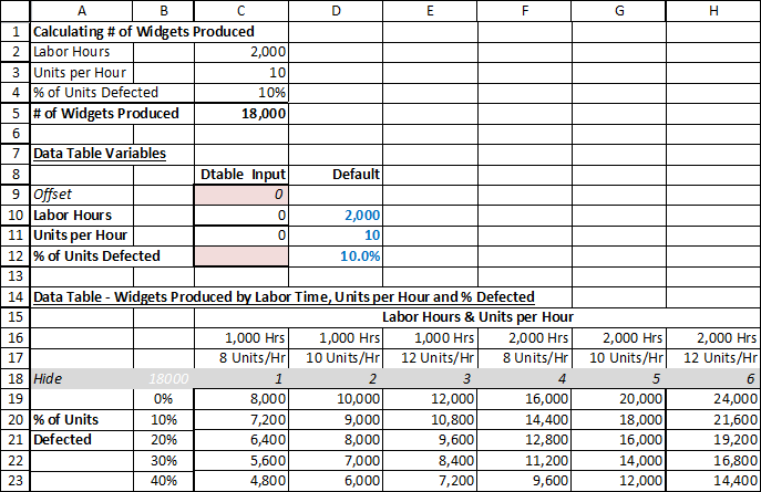
The key to making a three-variable data-table (or any higher number of variables, such as 4, 5, etc.) is to use the offset function to populate a set of values into the base calculation. (The data-table’s constraint of only having two variables remain unchanged.)
Setting Up the Model
There are three parts to this example:
- Rows 1 to 5. “Calculating # of Widgets Produced”:
- This is the “base model”, where the actual calculation occurs.
- # of Widgets Produced = labour hours times units per hour times % of units defected. Cells C2, C3 and C4 are possible inputs.
- C5 is the output we are looking for (# of Widgets Produced).
- Remember that all the data-table does is feed different possible input values to get answers for each scenario.
- Rows 7 to 12. “Data-Table Variables”: This is where the data table change actual cells to create different scenarios.
- Rows 14 to 23. “Data Table – Widgets Produced by Labor Time, Units per Hour, and % Defected”
Step by Step Explanation
- Data table changes cells C9, C12
- Row 18 are possible values for C9. (1, 2, 3, 4..6) Notice that these are not the actual values to be used to calculate # of widgets produced. Instead, C10 and C11 are actual values to calculate # of widgets produced. C10 and C11 uses C9’s value as the offset to pick up the correct hours and # units/hour values on rows 16 and 17.
- [C10] = OFFSET($B$16,0,$C$9)
Starting from Cell B16, Excel is to go to the cell on the right based on the value of Cell C9. So if C9 is 0, stay on current cell. If C9 is 3 then go 3 to the right, meaning E9. - [C11] = OFFSET($B$17,0,$C$9)
Similar logic.
- [C10] = OFFSET($B$16,0,$C$9)
- B19 to B23 are possible values for C12. (0%, 10%..40% Actual % values of defects.)
- D10, D11, D12 are defaults. This is what the formula in rows 2 to 5 show on the screen by default.
- [C2] =IF(‘3-Var Datatable’!C9=0,D10,’3-Var Datatable’!C10)
This means if C9=0 (by default it should be 0, since only the data table changes C9), formula should equal to the default “Labour Hours” value (stored in D10). Otherwise, if value is no 0 (meaning data table is calculating value), then it will use cell C10, which is some input value based on the data table. - [C3], [C4] is similar logic.
- [C2] =IF(‘3-Var Datatable’!C9=0,D10,’3-Var Datatable’!C10)
How to Change this Model for Your Purposes
- To use this model first you need to decide on the “Base model”. This includes:
- The required formula inputs
- The output you are looking to calculate
- And the formula of calculation.
- Input the default values for input cells – this is the base case.
- Decide on the combination of inputs that you want to perform the sensitivities on.
- There is no real limitations on the combinations, except consideration for how much data you want to present to the reader. You may want to be very comprehensive or brief depending on what you are using the file for.
- In the example above, we applied # of hours and units per hour as the column input. You can, of course, change that to fit your inputs.
- Decide on the values of inputs you want to calculate in the data table. In this example:
- The Labour Hours & Units per Hour section shows 1,000 and 2,000 hours combined with 8, 10, and 12 units per hour, resulting in 6 possible “scenarios”. It is possible to provide more granularity for labour hours (e.g. adding 1,500 hours), # of units per hour, etc.
- The % of units defected has a high range here (0% to 40%), as this is only an example to show you how a 3-variable data table can work. For practical purposes, you may want to narrow the range and provide better detail. Once again, the range of data table input values depends what type of situation you are dealing with.
- Make sure cell B18 is linked to cell C5 or the output cell for the “Base Model” section.
3 people found this article useful
3 people found this article useful
I have a dataset in an Excel sheet and i need to RANDOMLY split this (for instance 999 records) into 3 equal (and no duplicates) Excel files. Can this be done simply by using some Excel function or I need to write code to specifically do this?
asked Apr 28, 2015 at 17:21
![]()
user90790user90790
3051 gold badge4 silver badges13 bronze badges
1
Sometimes low-tech is best. If you don’t need to repeat this very frequently…
- add a column to the dataset, fill with
=RAND() - sort the dataset on this column
- copy the first 333 rows into a new sheet
- copy the next 333 rows into a new sheet
I bet that would take less time than you’ve already spent trying to get the macros to work.
answered Apr 29, 2015 at 9:11
![]()
aucupariaaucuparia
2,03118 silver badges27 bronze badges
1
This revised macro will take the original 999 records and randomly distribute them into three other files (each file containing exactly 333 items) :
Sub croupier()
    Dim k1 As Long, k2 As Long, k3 As Long
    Dim Original As Workbook
    Dim I As Long, ary(1 To 999)
    Set Original = ActiveWorkbook
    Dim rw As Long

    Workbooks.Add
    Set Winken = ActiveWorkbook
    Workbooks.Add
    Set Blinken = ActiveWorkbook
    Workbooks.Add
    Set Nod = ActiveWorkbook
    k1 = 1
    k2 = 1
    k3 = 1
    For I = 1 To 999
        ary(I) = I
    Next I

    Call Shuffle(ary)

    With Original.Sheets("Sheet1")
    For I = 1 To 333
        rw = ary(I)
        .Cells(rw, 1).EntireRow.Copy Winken.Sheets("Sheet1").Cells(k1, 1)
        k1 = k1 + 1
    Next I
    For I = 334 To 666
        rw = ary(I)
        .Cells(rw, 1).EntireRow.Copy Blinken.Sheets("Sheet1").Cells(k2, 1)
        k2 = k2 + 1
    Next I
    For I = 667 To 999
        rw = ary(I)
        .Cells(rw, 1).EntireRow.Copy Nod.Sheets("Sheet1").Cells(k3, 1)
        k3 = k3 + 1
    Next I
    End With

    Winken.Save
    Blinken.Save
    Nod.Save
    Winken.Close
    Blinken.Close
    Nod.Close

End Sub


Sub Shuffle(InOut() As Variant)
    Dim HowMany As Long, I As Long, J As Long
    Dim tempF As Double, temp As Variant

    Hi = UBound(InOut)
    Low = LBound(InOut)
    ReDim Helper(Low To Hi) As Double
    Randomize

    For I = Low To Hi
        Helper(I) = Rnd
    Next I


    J = (Hi - Low + 1)  2
    Do While J > 0
        For I = Low To Hi - J
          If Helper(I) > Helper(I + J) Then
            tempF = Helper(I)
            Helper(I) = Helper(I + J)
            Helper(I + J) = tempF
            temp = InOut(I)
            InOut(I) = InOut(I + J)
            InOut(I + J) = temp
          End If
        Next I
        For I = Hi - J To Low Step -1
          If Helper(I) > Helper(I + J) Then
            tempF = Helper(I)
            Helper(I) = Helper(I + J)
            Helper(I + J) = tempF
            temp = InOut(I)
            InOut(I) = InOut(I + J)
            InOut(I + J) = temp
          End If
        Next I
        J = J  2
    Loop
End Sub
answered Apr 28, 2015 at 19:02
![]()
Gary’s StudentGary’s Student
95.3k9 gold badges58 silver badges98 bronze badges
1
Here is a macro that will accept an array and copy to three different sheets:
Sub DoWork(Students As Variant)

Dim i As Long
Dim row As Integer
Dim sheetNumber As Integer
ReDim myArray(UBound(Students)) As Variant
Dim shuffledArray As Variant
Dim wkSheet As Worksheet
Dim myBooks(3) As Workbook

Set myBooks(1) = workBooks.Add
Set myBooks(2) = workBooks.Add
Set myBooks(3) = workBooks.Add

'populate the array with the number of rows
For i = 1 To UBound(Students)
    myArray(i) = i
Next

'shuffle the array to provide true randomness
shuffledArray = ShuffleArray(myArray)

sheetNumber = 1
row = 1

'loop through the rows assiging to sheets
For i = 1 To UBound(Students)

    If sheetNumber = 4 Then
        sheetNumber = 1
        row = row + 1
    End If

    Set wkSheet = myBooks(sheetNumber).ActiveSheet

    wkSheet.Cells(row, 1) = Students(shuffledArray(i))

    sheetNumber = sheetNumber + 1

Next

myBooks(1).SaveAs ("ws1.xlsx")
myBooks(2).SaveAs ("ws2.xlsx")
myBooks(3).SaveAs ("ws3.xlsx")

End Sub

Function ShuffleArray(InArray() As Variant) As Variant()
''''''''''''''''''''''''''''''''''''''''''''''''''''''''''''''''''''''''''''''''''''
' ShuffleArray
' This function returns the values of InArray in random order. The original
' InArray is not modified.
''''''''''''''''''''''''''''''''''''''''''''''''''''''''''''''''''''''''''''''''''''
    Dim N As Long
    Dim Temp As Variant
    Dim J As Long
    Dim Arr() As Variant
    Dim L As Long


    Randomize
    L = UBound(InArray) - LBound(InArray) + 1
    ReDim Arr(LBound(InArray) To UBound(InArray))
    For N = LBound(InArray) To UBound(InArray)
        Arr(N) = InArray(N)
    Next N
    For N = LBound(Arr) To UBound(Arr)
        J = CLng(((UBound(Arr) - N) * Rnd) + N)
        Temp = Arr(N)
        Arr(N) = Arr(J)
        Arr(J) = Temp
    Next N
    ShuffleArray = Arr
End Function

Sub ShuffleArrayInPlace(InArray() As Variant)
''''''''''''''''''''''''''''''''''''''''''''''''''''''''''''''''''''''''''''''''''''
' ShuffleArrayInPlace
' This shuffles InArray to random order, randomized in place.
''''''''''''''''''''''''''''''''''''''''''''''''''''''''''''''''''''''''''''''''''''
    Dim N As Long
    Dim L As Long
    Dim Temp As Variant
    Dim J As Long

    Randomize
    L = UBound(InArray) - LBound(InArray) + 1
    For N = LBound(InArray) To UBound(InArray)
        J = CLng(((UBound(InArray) - N) * Rnd) + N)
        If N <> J Then
            Temp = InArray(N)
            InArray(N) = InArray(J)
            InArray(J) = Temp
        End If
    Next N
End Sub
You would then call with something like this:
Option Explicit
Option Base 1

Sub Test()

Dim i As Long

Dim Students(999) As Variant

'populate the array with the number of rows
For i = 1 To UBound(Students)
    Students(i) = "Students-" & Str(i)
Next

DoWork (Students)

End Sub
answered Apr 28, 2015 at 19:14
![]()
KevinKevin
2,5461 gold badge11 silver badges12 bronze badges
0
Split text into different columns with functions
Excel for Microsoft 365 Excel for Microsoft 365 for Mac Excel for the web Excel 2021 Excel 2021 for Mac Excel 2019 Excel 2019 for Mac Excel 2016 Excel 2016 for Mac Excel 2013 Excel Web App Excel 2010 Excel 2007 Excel for Mac 2011 More…Less
You can use the LEFT, MID, RIGHT, SEARCH, and LEN text functions to manipulate strings of text in your data. For example, you can distribute the first, middle, and last names from a single cell into three separate columns.
The key to distributing name components with text functions is the position of each character within a text string. The positions of the spaces within the text string are also important because they indicate the beginning or end of name components in a string.
For example, in a cell that contains only a first and last name, the last name begins after the first instance of a space. Some names in your list may contain a middle name, in which case, the last name begins after the second instance of a space.
This article shows you how to extract various components from a variety of name formats using these handy functions. You can also split text into different columns with the Convert Text to Columns Wizard
|
Example name |
Description |
First name |
Middle name |
Last name |
Suffix |
|
|
1 |
Jeff Smith |
No middle name |
Jeff |
Smith |
||
|
2 |
Eric S. Kurjan |
One middle initial |
Eric |
S. |
Kurjan |
|
|
3 |
Janaina B. G. Bueno |
Two middle initials |
Janaina |
B. G. |
Bueno |
|
|
4 |
Kahn, Wendy Beth |
Last name first, with comma |
Wendy |
Beth |
Kahn |
|
|
5 |
Mary Kay D. Andersen |
Two-part first name |
Mary Kay |
D. |
Andersen |
|
|
6 |
Paula Barreto de Mattos |
Three-part last name |
Paula |
Barreto de Mattos |
||
|
7 |
James van Eaton |
Two-part last name |
James |
van Eaton |
||
|
8 |
Bacon Jr., Dan K. |
Last name and suffix first, with comma |
Dan |
K. |
Bacon |
Jr. |
|
9 |
Gary Altman III |
With suffix |
Gary |
Altman |
III |
|
|
10 |
Mr. Ryan Ihrig |
With prefix |
Ryan |
Ihrig |
||
|
11 |
Julie Taft-Rider |
Hyphenated last name |
Julie |
Taft-Rider |
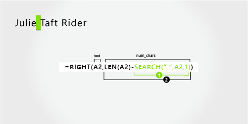
Note: In the graphics in the following examples, the highlight in the full name shows the character that the matching SEARCH formula is looking for.
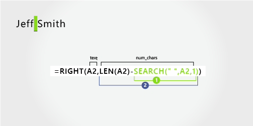
This example separates two components: first name and last name. A single space separates the two names.
Copy the cells in the table and paste into an Excel worksheet at cell A1. The formula you see on the left will be displayed for reference, while Excel will automatically convert the formula on the right into the appropriate result.
Hint Before you paste the data into the worksheet, set the column widths of columns A and B to 250.
|
Example name |
Description |
|
Jeff Smith |
No middle name |
|
Formula |
Result (first name) |
|
‘=LEFT(A2, SEARCH(» «,A2,1)) |
=LEFT(A2, SEARCH(» «,A2,1)) |
|
Formula |
Result (last name) |
|
‘=RIGHT(A2,LEN(A2)-SEARCH(» «,A2,1)) |
=RIGHT(A2,LEN(A2)-SEARCH(» «,A2,1)) |
-
First name
The first name starts with the first character in the string (J) and ends at the fifth character (the space). The formula returns five characters in cell A2, starting from the left.

Use the SEARCH function to find the value for num_chars:
Search for the numeric position of the space in A2, starting from the left.
-
Last name
The last name starts at the space, five characters from the right, and ends at the last character on the right (h). The formula extracts five characters in A2, starting from the right.
Use the SEARCH and LEN functions to find the value for num_chars:
Search for the numeric position of the space in A2, starting from the left. (5)
-
Count the total length of the text string, and then subtract the number of characters to the left of the first space, as found in step 1.

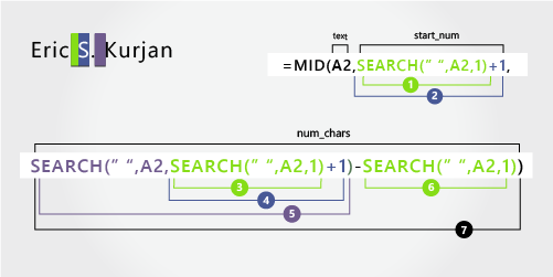
This example uses a first name, middle initial, and last name. A space separates each name component.
Copy the cells in the table and paste into an Excel worksheet at cell A1. The formula you see on the left will be displayed for reference, while Excel will automatically convert the formula on the right into the appropriate result.
Hint Before you paste the data into the worksheet, set the column widths of columns A and B to 250.
|
Example name |
Description |
|
Eric S. Kurjan |
One middle initial |
|
Formula |
Result (first name) |
|
‘=LEFT(A2, SEARCH(» «,A2,1)) |
=LEFT(A2, SEARCH(» «,A2,1)) |
|
Formula |
Result (middle initial) |
|
‘=MID(A2,SEARCH(» «,A2,1)+1,SEARCH(» «,A2,SEARCH(» «,A2,1)+1)-SEARCH(» «,A2,1)) |
=MID(A2,SEARCH(» «,A2,1)+1,SEARCH(» «,A2,SEARCH(» «,A2,1)+1)-SEARCH(» «,A2,1)) |
|
Formula |
Live Result (last name) |
|
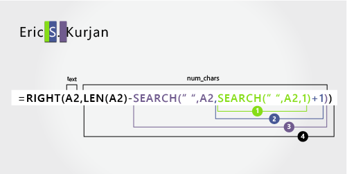
‘=RIGHT(A2,LEN(A2)-SEARCH(» «,A2,SEARCH(» «,A2,1)+1)) |
=RIGHT(A2,LEN(A2)-SEARCH(» «,A2,SEARCH(» «,A2,1)+1)) |
-
First name
The first name starts with the first character from the left (E) and ends at the fifth character (the first space). The formula extracts the first five characters in A2, starting from the left.
Use the SEARCH function to find the value for num_chars:
Search for the numeric position of the space in A2, starting from the left. (5)
-
Middle name
The middle name starts at the sixth character position (S), and ends at the eighth position (the second space). This formula involves nesting SEARCH functions to find the second instance of a space.
The formula extracts three characters, starting from the sixth position.
Use the SEARCH function to find the value for start_num:
Search for the numeric position of the first space in A2, starting from the first character from the left. (5).
-
Add 1 to get the position of the character after the first space (S). This numeric position is the starting position of the middle name. (5 + 1 = 6)
Use nested SEARCH functions to find the value for num_chars:
Search for the numeric position of the first space in A2, starting from the first character from the left. (5)
-
Add 1 to get the position of the character after the first space (S). The result is the character number at which you want to start searching for the second instance of space. (5 + 1 = 6)
-
Search for the second instance of space in A2, starting from the sixth position (S) found in step 4. This character number is the ending position of the middle name. (8)
-
Search for the numeric position of space in A2, starting from the first character from the left. (5)
-
Take the character number of the second space found in step 5 and subtract the character number of the first space found in step 6. The result is the number of characters MID extracts from the text string starting at the sixth position found in step 2. (8 – 5 = 3)
-
Last name
The last name starts six characters from the right (K) and ends at the first character from the right (n). This formula involves nesting SEARCH functions to find the second and third instances of a space (which are at the fifth and eighth positions from the left).
The formula extracts six characters in A2, starting from the right.
-
Use the LEN and nested SEARCH functions to find the value for num_chars:
Search for the numeric position of space in A2, starting from the first character from the left. (5)
-
Add 1 to get the position of the character after the first space (S). The result is the character number at which you want to start searching for the second instance of space. (5 + 1 = 6)
-
Search for the second instance of space in A2, starting from the sixth position (S) found in step 2. This character number is the ending position of the middle name. (8)
-
Count the total length of the text string in A2, and then subtract the number of characters from the left up to the second instance of space found in step 3. The result is the number of characters to be extracted from the right of the full name. (14 – 8 = 6).

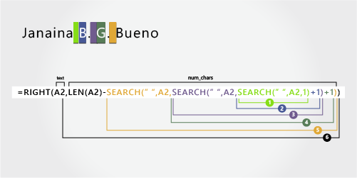
Here’s an example of how to extract two middle initials. The first and third instances of space separate the name components.
Copy the cells in the table and paste into an Excel worksheet at cell A1. The formula you see on the left will be displayed for reference, while Excel will automatically convert the formula on the right into the appropriate result.
Hint Before you paste the data into the worksheet, set the column widths of columns A and B to 250.
|
Example name |
Description |
|
Janaina B. G. Bueno |
Two middle initials |
|
Formula |
Result (first name) |
|
‘=LEFT(A2, SEARCH(» «,A2,1)) |
=LEFT(A2, SEARCH(» «,A2,1)) |
|
Formula |
Result (middle initials) |
|
‘=MID(A2,SEARCH(» «,A2,1)+1,SEARCH(» «,A2,SEARCH(» «,A2,SEARCH(» «,A2,1)+1)+1)-SEARCH(» «,A2,1)) |
=MID(A2,SEARCH(» «,A2,1)+1,SEARCH(» «,A2,SEARCH(» «,A2,SEARCH(» «,A2,1)+1)+1)-SEARCH(» «,A2,1)) |
|
Formula |
Live Result (last name) |
|
‘=RIGHT(A2,LEN(A2)-SEARCH(» «,A2,SEARCH(» «,A2,SEARCH(» «,A2,1)+1)+1)) |
=RIGHT(A2,LEN(A2)-SEARCH(» «,A2,SEARCH(» «,A2,SEARCH(» «,A2,1)+1)+1)) |
-
First name
The first name starts with the first character from the left (J) and ends at the eighth character (the first space). The formula extracts the first eight characters in A2, starting from the left.
Use the SEARCH function to find the value for num_chars:
Search for the numeric position of the first space in A2, starting from the left. (8)
-
Middle name
The middle name starts at the ninth position (B), and ends at the fourteenth position (the third space). This formula involves nesting SEARCH to find the first, second, and third instances of space in the eighth, eleventh, and fourteenth positions.
The formula extracts five characters, starting from the ninth position.
Use the SEARCH function to find the value for start_num:
Search for the numeric position of the first space in A2, starting from the first character from the left. (8)
-
Add 1 to get the position of the character after the first space (B). This numeric position is the starting position of the middle name. (8 + 1 = 9)
Use nested SEARCH functions to find the value for num_chars:
Search for the numeric position of the first space in A2, starting from the first character from the left. (8)
-
Add 1 to get the position of the character after the first space (B). The result is the character number at which you want to start searching for the second instance of space. (8 + 1 = 9)
-
Search for the second space in A2, starting from the ninth position (B) found in step 4. (11).
-
Add 1 to get the position of the character after the second space (G). This character number is the starting position at which you want to start searching for the third space. (11 + 1 = 12)
-
Search for the third space in A2, starting at the twelfth position found in step 6. (14)
-
Search for the numeric position of the first space in A2. (8)
-
Take the character number of the third space found in step 7 and subtract the character number of the first space found in step 6. The result is the number of characters MID extracts from the text string starting at the ninth position found in step 2.
-
Last name
The last name starts five characters from the right (B) and ends at the first character from the right (o). This formula involves nesting SEARCH to find the first, second, and third instances of space.
The formula extracts five characters in A2, starting from the right of the full name.
Use nested SEARCH and the LEN functions to find the value for the num_chars:
Search for the numeric position of the first space in A2, starting from the first character from the left. (8)
-
Add 1 to get the position of the character after the first space (B). The result is the character number at which you want to start searching for the second instance of space. (8 + 1 = 9)
-
Search for the second space in A2, starting from the ninth position (B) found in step 2. (11)
-
Add 1 to get the position of the character after the second space (G). This character number is the starting position at which you want to start searching for the third instance of space. (11 + 1 = 12)
-
Search for the third space in A2, starting at the twelfth position (G) found in step 6. (14)
-
Count the total length of the text string in A2, and then subtract the number of characters from the left up to the third space found in step 5. The result is the number of characters to be extracted from the right of the full name. (19 — 14 = 5)


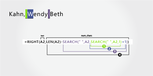
In this example, the last name comes before the first, and the middle name appears at the end. The comma marks the end of the last name, and a space separates each name component.
Copy the cells in the table and paste into an Excel worksheet at cell A1. The formula you see on the left will be displayed for reference, while Excel will automatically convert the formula on the right into the appropriate result.
Hint Before you paste the data into the worksheet, set the column widths of columns A and B to 250.
|
Example name |
Description |
|
Kahn, Wendy Beth |
Last name first, with comma |
|
Formula |
Result (first name) |
|
‘=MID(A2,SEARCH(» «,A2,1)+1,SEARCH(» «,A2,SEARCH(» «,A2,1)+1)-SEARCH(» «,A2,1)) |
=MID(A2,SEARCH(» «,A2,1)+1,SEARCH(» «,A2,SEARCH(» «,A2,1)+1)-SEARCH(» «,A2,1)) |
|
Formula |
Result (middle name) |
|
‘=RIGHT(A2,LEN(A2)-SEARCH(» «,A2,SEARCH(» «,A2,1)+1)) |
=RIGHT(A2,LEN(A2)-SEARCH(» «,A2,SEARCH(» «,A2,1)+1)) |
|
Formula |
Live Result (last name) |
|
‘=LEFT(A2, SEARCH(» «,A2,1)-2) |
=LEFT(A2, SEARCH(» «,A2,1)-2) |
-
First name
The first name starts with the seventh character from the left (W) and ends at the twelfth character (the second space). Because the first name occurs at the middle of the full name, you need to use the MID function to extract the first name.
The formula extracts six characters, starting from the seventh position.
Use the SEARCH function to find the value for start_num:
Search for the numeric position of the first space in A2, starting from the first character from the left. (6)
-
Add 1 to get the position of the character after the first space (W). This numeric position is the starting position of the first name. (6 + 1 = 7)
Use nested SEARCH functions to find the value for num_chars:
Search for the numeric position of the first space in A2, starting from the first character from the left. (6)
-
Add 1 to get the position of the character after the first space (W). The result is the character number at which you want to start searching for the second space. (6 + 1 = 7)
Search for the second space in A2, starting from the seventh position (W) found in step 4. (12)
-
Search for the numeric position of the first space in A2, starting from the first character from the left. (6)
-
Take the character number of the second space found in step 5 and subtract the character number of the first space found in step 6. The result is the number of characters MID extracts from the text string starting at the seventh position found in step 2. (12 — 6 = 6)
-
Middle name
The middle name starts four characters from the right (B), and ends at the first character from the right (h). This formula involves nesting SEARCH to find the first and second instances of space in the sixth and twelfth positions from the left.
The formula extracts four characters, starting from the right.
Use nested SEARCH and the LEN functions to find the value for start_num:
Search for the numeric position of the first space in A2, starting from the first character from the left. (6)
-
Add 1 to get the position of the character after the first space (W). The result is the character number at which you want to start searching for the second space. (6 + 1 = 7)
-
Search for the second instance of space in A2 starting from the seventh position (W) found in step 2. (12)
-
Count the total length of the text string in A2, and then subtract the number of characters from the left up to the second space found in step 3. The result is the number of characters to be extracted from the right of the full name. (16 — 12 = 4)
-
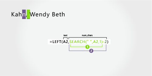
Last name
The last name starts with the first character from the left (K) and ends at the fourth character (n). The formula extracts four characters, starting from the left.
Use the SEARCH function to find the value for num_chars:
Search for the numeric position of the first space in A2, starting from the first character from the left. (6)
-
Subtract 2 to get the numeric position of the ending character of the last name (n). The result is the number of characters you want LEFT to extract. (6 — 2 =4)

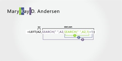
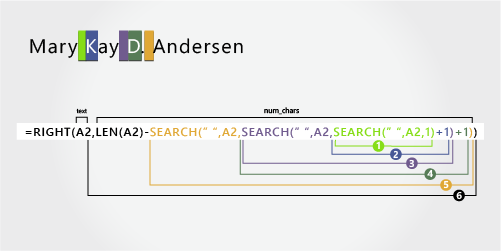
This example uses a two-part first name, Mary Kay. The second and third spaces separate each name component.
Copy the cells in the table and paste into an Excel worksheet at cell A1. The formula you see on the left will be displayed for reference, while Excel will automatically convert the formula on the right into the appropriate result.
Hint Before you paste the data into the worksheet, set the column widths of columns A and B to 250.
|
Example name |
Description |
|
Mary Kay D. Andersen |
Two-part first name |
|
Formula |
Result (first name) |
|
LEFT(A2, SEARCH(» «,A2,SEARCH(» «,A2,1)+1)) |
=LEFT(A2, SEARCH(» «,A2,SEARCH(» «,A2,1)+1)) |
|
Formula |
Result (middle initial) |
|
‘=MID(A2,SEARCH(» «,A2,SEARCH(» «,A2,1)+1)+1,SEARCH(» «,A2,SEARCH(» «,A2,SEARCH(» «,A2,1)+1)+1)-(SEARCH(» «,A2,SEARCH(» «,A2,1)+1)+1)) |
=MID(A2,SEARCH(» «,A2,SEARCH(» «,A2,1)+1)+1,SEARCH(» «,A2,SEARCH(» «,A2,SEARCH(» «,A2,1)+1)+1)-(SEARCH(» «,A2,SEARCH(» «,A2,1)+1)+1)) |
|
Formula |
Live Result (last name) |
|
‘=RIGHT(A2,LEN(A2)-SEARCH(» «,A2,SEARCH(» «,A2,SEARCH(» «,A2,1)+1)+1)) |
=RIGHT(A2,LEN(A2)-SEARCH(» «,A2,SEARCH(» «,A2,SEARCH(» «,A2,1)+1)+1)) |
-
First name
The first name starts with the first character from the left and ends at the ninth character (the second space). This formula involves nesting SEARCH to find the second instance of space from the left.
The formula extracts nine characters, starting from the left.
Use nested SEARCH functions to find the value for num_chars:
Search for the numeric position of the first space in A2, starting from the first character from the left. (5)
-
Add 1 to get the position of the character after the first space (K). The result is the character number at which you want to start searching for the second instance of space. (5 + 1 = 6)
-
Search for the second instance of space in A2, starting from the sixth position (K) found in step 2. The result is the number of characters LEFT extracts from the text string. (9)
-
Middle name
The middle name starts at the tenth position (D), and ends at the twelfth position (the third space). This formula involves nesting SEARCH to find the first, second, and third instances of space.
The formula extracts two characters from the middle, starting from the tenth position.
Use nested SEARCH functions to find the value for start_num:
Search for the numeric position of the first space in A2, starting from the first character from the left. (5)
-
Add 1 to get the character after the first space (K). The result is the character number at which you want to start searching for the second space. (5 + 1 = 6)
-
Search for the position of the second instance of space in A2, starting from the sixth position (K) found in step 2. The result is the number of characters LEFT extracts from the left. (9)
-
Add 1 to get the character after the second space (D). The result is the starting position of the middle name. (9 + 1 = 10)
Use nested SEARCH functions to find the value for num_chars:
Search for the numeric position of the character after the second space (D). The result is the character number at which you want to start searching for the third space. (10)
-
Search for the numeric position of the third space in A2, starting from the left. The result is the ending position of the middle name. (12)
-
Search for the numeric position of the character after the second space (D). The result is the beginning position of the middle name. (10)
-
Take the character number of the third space, found in step 6, and subtract the character number of “D”, found in step 7. The result is the number of characters MID extracts from the text string starting at the tenth position found in step 4. (12 — 10 = 2)
-
Last name
The last name starts eight characters from the right. This formula involves nesting SEARCH to find the first, second, and third instances of space in the fifth, ninth, and twelfth positions.
The formula extracts eight characters from the right.
Use nested SEARCH and the LEN functions to find the value for num_chars:
Search for the numeric position of the first space in A2, starting from the left. (5)
-
Add 1 to get the character after the first space (K). The result is the character number at which you want to start searching for the space. (5 + 1 = 6)
-
Search for the second space in A2, starting from the sixth position (K) found in step 2. (9)
-
Add 1 to get the position of the character after the second space (D). The result is the starting position of the middle name. (9 + 1 = 10)
-
Search for the numeric position of the third space in A2, starting from the left. The result is the ending position of the middle name. (12)
-
Count the total length of the text string in A2, and then subtract the number of characters from the left up to the third space found in step 5. The result is the number of characters to be extracted from the right of the full name. (20 — 12 =


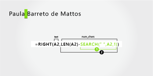
This example uses a three-part last name: Barreto de Mattos. The first space marks the end of the first name and the beginning of the last name.
Copy the cells in the table and paste into an Excel worksheet at cell A1. The formula you see on the left will be displayed for reference, while Excel will automatically convert the formula on the right into the appropriate result.
Hint Before you paste the data into the worksheet, set the column widths of columns A and B to 250.
|
Example name |
Description |
|
Paula Barreto de Mattos |
Three-part last name |
|
Formula |
Result (first name) |
|
‘=LEFT(A2, SEARCH(» «,A2,1)) |
=LEFT(A2, SEARCH(» «,A2,1)) |
|
Formula |
Result (last name) |
|
RIGHT(A2,LEN(A2)-SEARCH(» «,A2,1)) |
=RIGHT(A2,LEN(A2)-SEARCH(» «,A2,1)) |
-
First name
The first name starts with the first character from the left (P) and ends at the sixth character (the first space). The formula extracts six characters from the left.
Use the Search function to find the value for num_chars:
Search for the numeric position of the first space in A2, starting from the left. (6)
-
Last name
The last name starts seventeen characters from the right (B) and ends with first character from the right (s). The formula extracts seventeen characters from the right.
Use the LEN and SEARCH functions to find the value for num_chars:
Search for the numeric position of the first space in A2, starting from the left. (6)
-
Count the total length of the text string in A2, and then subtract the number of characters from the left up to the first space, found in step 1. The result is the number of characters to be extracted from the right of the full name. (23 — 6 = 17)

This example uses a two-part last name: van Eaton. The first space marks the end of the first name and the beginning of the last name.
Copy the cells in the table and paste into an Excel worksheet at cell A1. The formula you see on the left will be displayed for reference, while Excel will automatically convert the formula on the right into the appropriate result.
Hint Before you paste the data into the worksheet, set the column widths of columns A and B to 250.
|
Example name |
Description |
|
James van Eaton |
Two-part last name |
|
Formula |
Result (first name) |
|
‘=LEFT(A2, SEARCH(» «,A2,1)) |
=LEFT(A2, SEARCH(» «,A2,1)) |
|
Formula |
Result (last name) |
|
‘=RIGHT(A2,LEN(A2)-SEARCH(» «,A2,1)) |
=RIGHT(A2,LEN(A2)-SEARCH(» «,A2,1)) |
-
First name
The first name starts with the first character from the left (J) and ends at the eighth character (the first space). The formula extracts six characters from the left.
Use the SEARCH function to find the value for num_chars:
Search for the numeric position of the first space in A2, starting from the left. (6)
-
Last name
The last name starts with the ninth character from the right (v) and ends at the first character from the right (n). The formula extracts nine characters from the right of the full name.
Use the LEN and SEARCH functions to find the value for num_chars:
Search for the numeric position of the first space in A2, starting from the left. (6)
-
Count the total length of the text string in A2, and then subtract the number of characters from the left up to the first space, found in step 1. The result is the number of characters to be extracted from the right of the full name. (15 — 6 = 9)


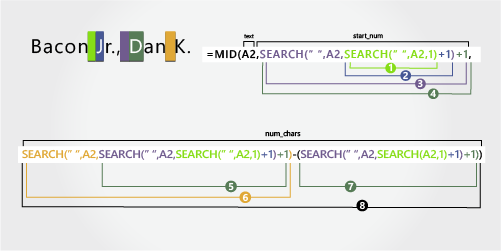
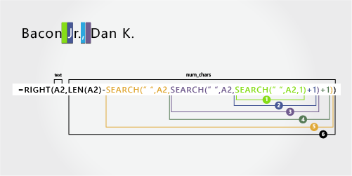
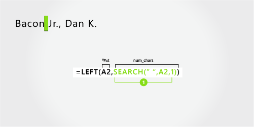
In this example, the last name comes first, followed by the suffix. The comma separates the last name and suffix from the first name and middle initial.
Copy the cells in the table and paste into an Excel worksheet at cell A1. The formula you see on the left will be displayed for reference, while Excel will automatically convert the formula on the right into the appropriate result.
Hint Before you paste the data into the worksheet, set the column widths of columns A and B to 250.
|
Example name |
Description |
|
Bacon Jr., Dan K. |
Last name and suffix first, with comma |
|
Formula |
Result (first name) |
|
‘=MID(A2,SEARCH(» «,A2,SEARCH(» «,A2,1)+1)+1,SEARCH(» «,A2,SEARCH(» «,A2,SEARCH(» «,A2,1)+1)+1)-SEARCH(» «,A2,SEARCH(» «,A2,1)+1)) |
=MID(A2,SEARCH(» «,A2,SEARCH(» «,A2,1)+1)+1,SEARCH(» «,A2,SEARCH(» «,A2,SEARCH(» «,A2,1)+1)+1)-SEARCH(» «,A2,SEARCH(» «,A2,1)+1)) |
|
Formula |
Result (middle initial) |
|
‘=RIGHT(A2,LEN(A2)-SEARCH(» «,A2,SEARCH(» «,A2,SEARCH(» «,A2,1)+1)+1)) |
=RIGHT(A2,LEN(A2)-SEARCH(» «,A2,SEARCH(» «,A2,SEARCH(» «,A2,1)+1)+1)) |
|
Formula |
Result (last name) |
|
‘=LEFT(A2, SEARCH(» «,A2,1)) |
=LEFT(A2, SEARCH(» «,A2,1)) |
|
Formula |
Result (suffix) |
|
‘=MID(A2,SEARCH(» «, A2,1)+1,(SEARCH(» «,A2,SEARCH(» «,A2,1)+1)-2)-SEARCH(» «,A2,1)) |
=MID(A2,SEARCH(» «, A2,1)+1,(SEARCH(» «,A2,SEARCH(» «,A2,1)+1)-2)-SEARCH(» «,A2,1)) |
-
First name
The first name starts with the twelfth character (D) and ends with the fifteenth character (the third space). The formula extracts three characters, starting from the twelfth position.
Use nested SEARCH functions to find the value for start_num:
Search for the numeric position of the first space in A2, starting from the left. (6)
-
Add 1 to get the character after the first space (J). The result is the character number at which you want to start searching for the second space. (6 + 1 = 7)
-
Search for the second space in A2, starting from the seventh position (J), found in step 2. (11)
-
Add 1 to get the character after the second space (D). The result is the starting position of the first name. (11 + 1 = 12)
Use nested SEARCH functions to find the value for num_chars:
Search for the numeric position of the character after the second space (D). The result is the character number at which you want to start searching for the third space. (12)
-
Search for the numeric position of the third space in A2, starting from the left. The result is the ending position of the first name. (15)
-
Search for the numeric position of the character after the second space (D). The result is the beginning position of the first name. (12)
-
Take the character number of the third space, found in step 6, and subtract the character number of “D”, found in step 7. The result is the number of characters MID extracts from the text string starting at the twelfth position, found in step 4. (15 — 12 = 3)
-
Middle name
The middle name starts with the second character from the right (K). The formula extracts two characters from the right.
Search for the numeric position of the first space in A2, starting from the left. (6)
-
Add 1 to get the character after the first space (J). The result is the character number at which you want to start searching for the second space. (6 + 1 = 7)
-
Search for the second space in A2, starting from the seventh position (J), found in step 2. (11)
-
Add 1 to get the character after the second space (D). The result is the starting position of the first name. (11 + 1 = 12)
-
Search for the numeric position of the third space in A2, starting from the left. The result is the ending position of the middle name. (15)
-
Count the total length of the text string in A2, and then subtract the number of characters from the left up to the third space, found in step 5. The result is the number of characters to be extracted from the right of the full name. (17 — 15 = 2)
-
Last name
The last name starts at the first character from the left (B) and ends at sixth character (the first space). Therefore, the formula extracts six characters from the left.
Use the SEARCH function to find the value for num_chars:
Search for the numeric position of the first space in A2, starting from the left. (6)
-
Suffix
The suffix starts at the seventh character from the left (J), and ends at ninth character from the left (.). The formula extracts three characters, starting from the seventh character.
Use the SEARCH function to find the value for start_num:
Search for the numeric position of the first space in A2, starting from the left. (6)
-
Add 1 to get the character after the first space (J). The result is the starting position of the suffix. (6 + 1 = 7)
Use nested SEARCH functions to find the value for num_chars:
Search for the numeric position of the first space in A2, starting from the left. (6)
-
Add 1 to get the numeric position of the character after the first space (J). The result is the character number at which you want to start searching for the second space. (7)
-
Search for the numeric position of the second space in A2, starting from the seventh character found in step 4. (11)
-
Subtract 1 from the character number of the second space found in step 4 to get the character number of “,”. The result is the ending position of the suffix. (11 — 1 = 10)
-
Search for the numeric position of the first space. (6)
-
After finding the first space, add 1 to find the next character (J), also found in steps 3 and 4. (7)
-
Take the character number of “,” found in step 6, and subtract the character number of “J”, found in steps 3 and 4. The result is the number of characters MID extracts from the text string starting at the seventh position, found in step 2. (10 — 7 = 3)

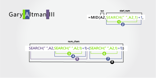
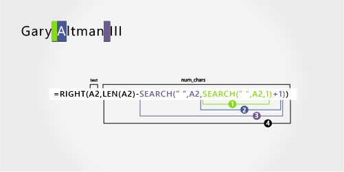
In this example, the first name is at the beginning of the string and the suffix is at the end, so you can use formulas similar to Example 2: Use the LEFT function to extract the first name, the MID function to extract the last name, and the RIGHT function to extract the suffix.
Copy the cells in the table and paste into an Excel worksheet at cell A1. The formula you see on the left will be displayed for reference, while Excel will automatically convert the formula on the right into the appropriate result.
Hint Before you paste the data into the worksheet, set the column widths of columns A and B to 250.
|
Example name |
Description |
|
Gary Altman III |
First and last name with suffix |
|
Formula |
Result (first name) |
|
‘=LEFT(A2, SEARCH(» «,A2,1)) |
=LEFT(A2, SEARCH(» «,A2,1)) |
|
Formula |
Result (last name) |
|
‘=MID(A2,SEARCH(» «,A2,1)+1,SEARCH(» «,A2,SEARCH(» «,A2,1)+1)-(SEARCH(» «,A2,1)+1)) |
=MID(A2,SEARCH(» «,A2,1)+1,SEARCH(» «,A2,SEARCH(» «,A2,1)+1)-(SEARCH(» «,A2,1)+1)) |
|
Formula |
Result (suffix) |
|
‘=RIGHT(A2,LEN(A2)-SEARCH(» «,A2,SEARCH(» «,A2,1)+1)) |
=RIGHT(A2,LEN(A2)-SEARCH(» «,A2,SEARCH(» «,A2,1)+1)) |
-
First name
The first name starts at the first character from the left (G) and ends at the fifth character (the first space). Therefore, the formula extracts five characters from the left of the full name.
Search for the numeric position of the first space in A2, starting from the left. (5)
-
Last name
The last name starts at the sixth character from the left (A) and ends at the eleventh character (the second space). This formula involves nesting SEARCH to find the positions of the spaces.
The formula extracts six characters from the middle, starting from the sixth character.
Use the SEARCH function to find the value for start_num:
Search for the numeric position of the first space in A2, starting from the left. (5)
-
Add 1 to get the position of the character after the first space (A). The result is the starting position of the last name. (5 + 1 = 6)
Use nested SEARCH functions to find the value for num_chars:
Search for the numeric position of the first space in A2, starting from the left. (5)
-
Add 1 to get the position of the character after the first space (A). The result is the character number at which you want to start searching for the second space. (5 + 1 = 6)
-
Search for the numeric position of the second space in A2, starting from the sixth character found in step 4. This character number is the ending position of the last name. (12)
-
Search for the numeric position of the first space. (5)
-
Add 1 to find the numeric position of the character after the first space (A), also found in steps 3 and 4. (6)
-
Take the character number of the second space, found in step 5, and then subtract the character number of “A”, found in steps 6 and 7. The result is the number of characters MID extracts from the text string, starting at the sixth position, found in step 2. (12 — 6 = 6)
-
Suffix
The suffix starts three characters from the right. This formula involves nesting SEARCH to find the positions of the spaces.
Use nested SEARCH and the LEN functions to find the value for num_chars:
Search for the numeric position of the first space in A2, starting from the left. (5)
-
Add 1 to get the character after the first space (A). The result is the character number at which you want to start searching for the second space. (5 + 1 = 6)
-
Search for the second space in A2, starting from the sixth position (A), found in step 2. (12)
-
Count the total length of the text string in A2, and then subtract the number of characters from the left up to the second space, found in step 3. The result is the number of characters to be extracted from the right of the full name. (15 — 12 = 3)

In this example, the full name is preceded by a prefix, and you use formulas similar to Example 2: the MID function to extract the first name, the RIGHT function to extract the last name.
Copy the cells in the table and paste into an Excel worksheet at cell A1. The formula you see on the left will be displayed for reference, while Excel will automatically convert the formula on the right into the appropriate result.
Hint Before you paste the data into the worksheet, set the column widths of columns A and B to 250.
|
Example name |
Description |
|
Mr. Ryan Ihrig |
With prefix |
|
Formula |
Result (first name) |
|
‘=MID(A2,SEARCH(» «,A2,1)+1,SEARCH(» «,A2,SEARCH(» «,A2,1)+1)-(SEARCH(» «,A2,1)+1)) |
=MID(A2,SEARCH(» «,A2,1)+1,SEARCH(» «,A2,SEARCH(» «,A2,1)+1)-(SEARCH(» «,A2,1)+1)) |
|
Formula |
Result (last name) |
|
‘=RIGHT(A2,LEN(A2)-SEARCH(» «,A2,SEARCH(» «,A2,1)+1)) |
=RIGHT(A2,LEN(A2)-SEARCH(» «,A2,SEARCH(» «,A2,1)+1)) |
-
First name
The first name starts at the fifth character from the left (R) and ends at the ninth character (the second space). The formula nests SEARCH to find the positions of the spaces. It extracts four characters, starting from the fifth position.
Use the SEARCH function to find the value for the start_num:
Search for the numeric position of the first space in A2, starting from the left. (4)
-
Add 1 to get the position of the character after the first space (R). The result is the starting position of the first name. (4 + 1 = 5)
Use nested SEARCH function to find the value for num_chars:
Search for the numeric position of the first space in A2, starting from the left. (4)
-
Add 1 to get the position of the character after the first space (R). The result is the character number at which you want to start searching for the second space. (4 + 1 = 5)
-
Search for the numeric position of the second space in A2, starting from the fifth character, found in steps 3 and 4. This character number is the ending position of the first name. (9)
-
Search for the first space. (4)
-
Add 1 to find the numeric position of the character after the first space (R), also found in steps 3 and 4. (5)
-
Take the character number of the second space, found in step 5, and then subtract the character number of “R”, found in steps 6 and 7. The result is the number of characters MID extracts from the text string, starting at the fifth position found in step 2. (9 — 5 = 4)
-
Last name
The last name starts five characters from the right. This formula involves nesting SEARCH to find the positions of the spaces.
Use nested SEARCH and the LEN functions to find the value for num_chars:
Search for the numeric position of the first space in A2, starting from the left. (4)
-
Add 1 to get the position of the character after the first space (R). The result is the character number at which you want to start searching for the second space. (4 + 1 = 5)
-
Search for the second space in A2, starting from the fifth position (R), found in step 2. (9)
-
Count the total length of the text string in A2, and then subtract the number of characters from the left up to the second space, found in step 3. The result is the number of characters to be extracted from the right of the full name. (14 — 9 = 5)


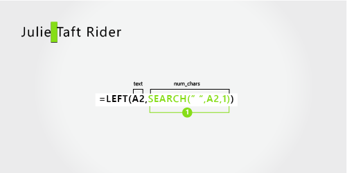
This example uses a hyphenated last name. A space separates each name component.
Copy the cells in the table and paste into an Excel worksheet at cell A1. The formula you see on the left will be displayed for reference, while Excel will automatically convert the formula on the right into the appropriate result.
Hint Before you paste the data into the worksheet, set the column widths of columns A and B to 250.
|
Example name |
Description |
|
Julie Taft-Rider |
Hyphenated last name |
|
Formula |
Result (first name) |
|
‘=LEFT(A2, SEARCH(» «,A2,1)) |
=LEFT(A2, SEARCH(» «,A2,1)) |
|
Formula |
Result (last name) |
|
‘=RIGHT(A2,LEN(A2)-SEARCH(» «,A2,1)) |
=RIGHT(A2,LEN(A2)-SEARCH(» «,A2,1)) |
-
First name
The first name starts at the first character from the left and ends at the sixth position (the first space). The formula extracts six characters from the left.
Use the SEARCH function to find the value of num_chars:
Search for the numeric position of the first space in A2, starting from the left. (6)
-
Last name
The entire last name starts ten characters from the right (T) and ends at the first character from the right (r).
Use the LEN and SEARCH functions to find the value for num_chars:
Search for the numeric position of the space in A2, starting from the first character from the left. (6)
-
Count the total length of the text string to be extracted, and then subtract the number of characters from the left up to the first space, found in step 1. (16 — 6 = 10)
Need more help?
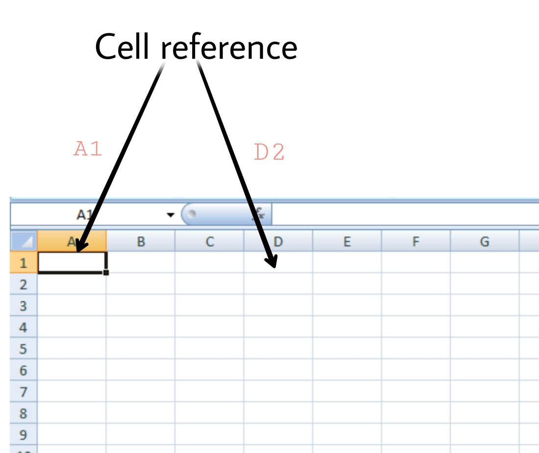
MS-EXCEL is a part of Microsoft Office suite software. It is an electronic spreadsheet with numerous rows and columns, used for organizing data, graphically represent data(s), and performing different calculations. It consists of 1048576 rows and 16384 columns, a row and column together make a cell. Each cell has an address defined by column name and row number example A1, D2, etc. this is also known as a cell reference.
Cell references: The address or name of a cell or a range of cells is known as Cell reference. It helps the software to identify the cell from where the data/value is to be used in the formula. We can reference the cell of other worksheets and also of other programs.
- Referencing the cell of other worksheets is known as External referencing.
- Referencing the cell of other programs is known as Remote referencing.
There are three types of cell references in Excel:
- Relative reference.
- Absolute reference.
- Mixed reference.
The Ribbon in MS-Excel is the topmost row of tabs that provide the user with different facilities/functionalities. These tabs are:

- Home Tab: It provides the basic facilities like changing the font, size of text, editing the cells in the spreadsheet, autosum, etc.
- Insert Tab: It provides the facilities like inserting tables, pivot tables, images, clip art, charts, links, etc.
- Page layout: It provides all the facilities related to the spreadsheet-like margins, orientation, height, width, background etc. The worksheet appearance will be the same in the hard copy as well.
- Formulas: It is a package of different in-built formulas/functions which can be used by user just by selecting the cell or range of cells for values.
- Data: The Data Tab helps to perform different operations on a vast set of data like analysis through what-if analysis tools and many other data analysis tools, removing duplicate data, transpose the row and column, etc. It also helps to access data(s) from different sources as well, such as from Ms-Access, from web, etc.
- Review: This tab provides the facility of thesaurus, checking spellings, translating the text, and helps to protect and share the worksheet and workbook.
- View: It contains the commands to manage the view of the workbook, show/hide ruler, gridlines, etc, freezing panes, and adding macros.
Creating a new spreadsheet:
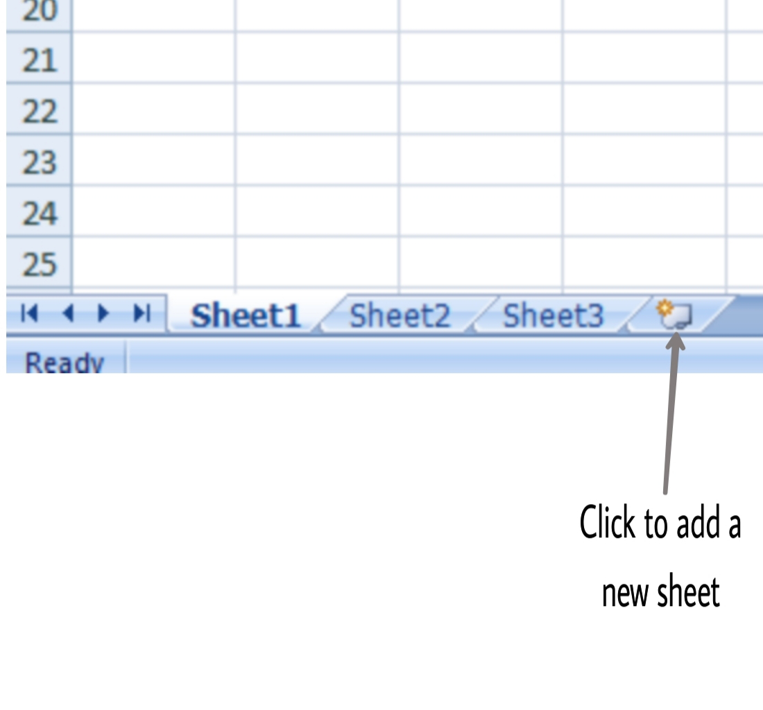
In Excel 3 sheets are already opened by default, now to add a new sheet :
- In the lowermost pane in Excel, you can find a button.
- Click on that button to add a new sheet.
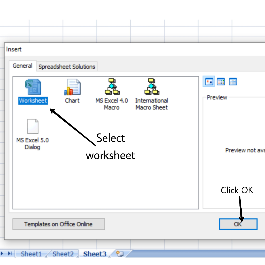
- We can also achieve the same by Right-clicking on the sheet number before which you want to insert the sheet.
- Click on Insert.
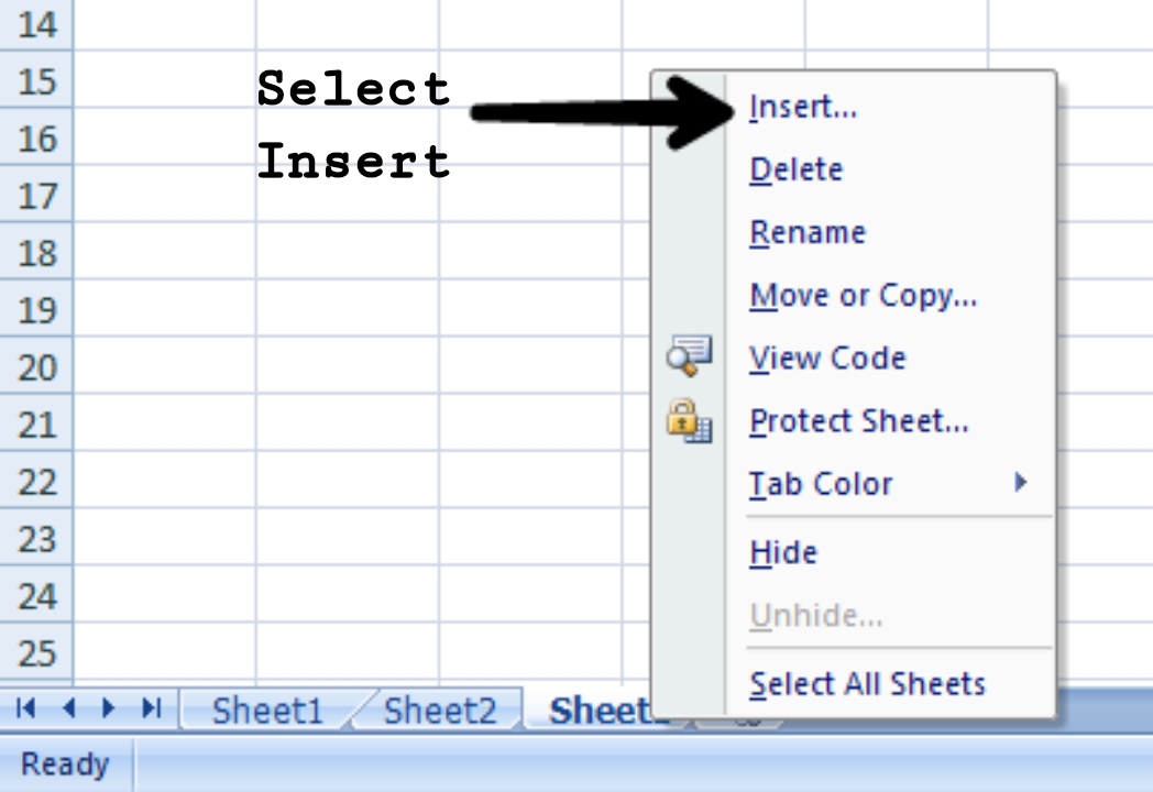
- Select Worksheet.
- Click OK.
Opening previous spreadsheet:
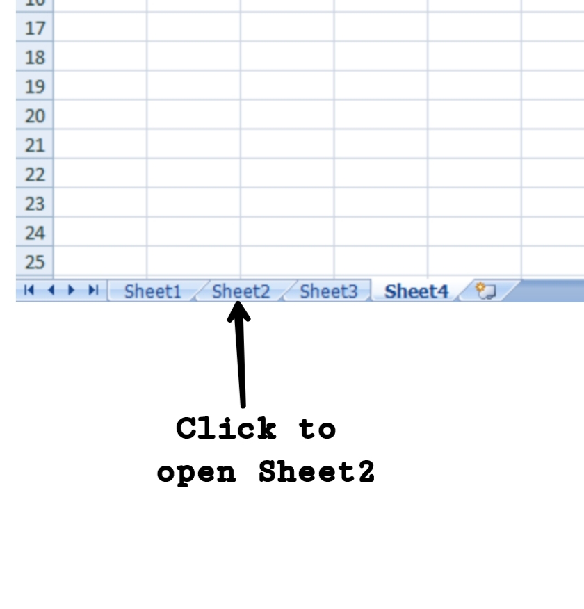
On the lowermost pane in Excel, you can find the name of the current sheet you have opened.
On the left side of this sheet, the name of previous sheets are also available like Sheet 2, Sheet 3 will be available at the left of sheet4, click on the number/name of the sheet you want to open and the sheet will open in the same workbook.
For example, we are on Sheet 4, and we want to open Sheet 2 then simply just click on Sheet2 to open it.
Managing the spreadsheets:
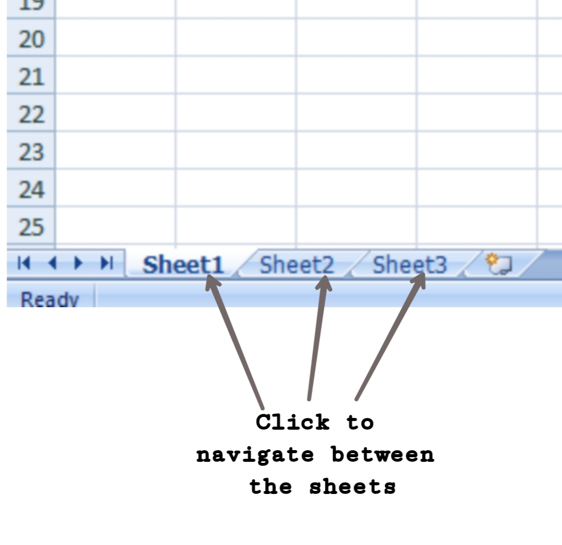
You can easily manage the spreadsheets in Excel simply by :
- Simply navigating between the sheets.
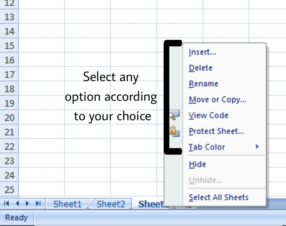
- Right-clicking on the sheet name or number on the pane.
- Choose among the various options available like, move, copy, rename, add, delete etc.
- You can move/copy your sheet to other workbooks as well just by selecting the workbook in the To workbook and the sheet before you want to insert the sheet in Before sheet.
To save the workbook:
- Click on the Office Button or the File tab.
- Click on Save As option.
- Write the desired name of your file.
- Click OK.
To share your workbook:
- Click on the Review tab on the Ribbon.
- Click on the share workbook (under Changes group).
- If you want to protect your workbook and then make it available for another user then click on Protect and Share Workbook option.
- Now check the option “Allow changes by more than one user at the same time. This also allows workbook merging” in the Share Workbook dialog box.
- Many other options are also available in the Advanced like track, update changes.
- Click OK.
Ms-Excel shortcuts:
- Ctrl+N: To open a new workbook.
- Ctrl+O: To open a saved workbook.
- Ctrl+S: To save a workbook.
- Ctrl+C: To copy the selected cells.
- Ctrl+V: To paste the copied cells.
- Ctrl+X: To cut the selected cells.
- Ctrl+W: To close the workbook.
- Delete: To remove all the contents from the cell.
- Ctrl+P: To print the workbook.
- Ctrl+Z: To undo.
This tutorial about cell format types in Excel is an essential part of your learning of Excel and will definitely do a lot of good to you in your future use of this software, as a lot of tasks in Excel sheets are based on cells format, as well as several errors are due to a bad implementation of it.
A good comprehension of the cell format types will build your knowledge on a solid basis to master Excel basics and will considerably save you time and effort when any related issue occurs.
A- Introduction
Excel software formats the cells depending on what type of information they contain.
To update the format of the highlighted cell, go to the “Home” tab of the ribbon and click, in the “Number” group of commands on the “Number Format” drop-down list.
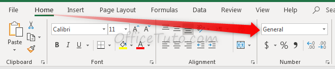
The drop-down list allows the selection to be changed.
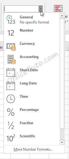
Cell formatting options in the “Number Format” drop-down list are:
- General
- Number
- Currency
- Accounting
- Short Date
- Long Date
- Time
- Percentage
- Fraction
- Scientific
- Text
- And the “More Number Formats” option.
Clicking the “More Number Formats” option brings up additional options for formatting cells, including the ability to do special and custom formatting options.
These options are discussed in detail in the below sections.
Cell format types in Excel are: General, Number, Currency, Accounting, Date, Time, Percentage, Fraction, Scientific, Text, Special (Zip Code, Zip Code + 4, Phone Number, Social Security Number), and Custom. You can get them from the “Number Format” drop-down list in the “Home” tab, or from the launcher arrow below it.
I will detail each one of them in the following sections:
1- General format
By default, cells are formatted as “General”, which could store any type of information. The General format means that no specific format is applied to the selected cell.
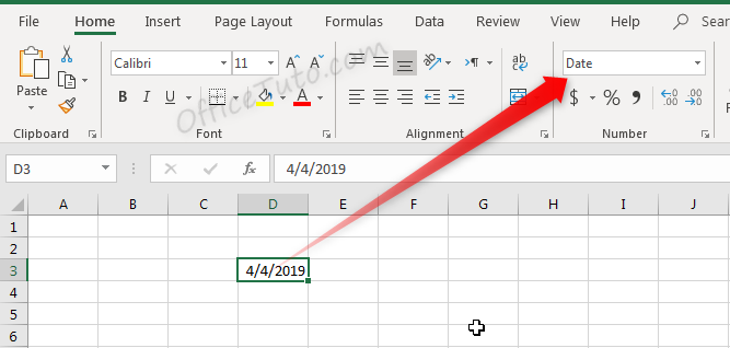
When information is typed into a cell, the cell format may change automatically. For example, if I enter “4/4/19” into a cell and press enter, then highlight the cell to view details about it, the cell format will be listed as “Date” instead of “General”.
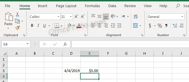
Similarly, we can update a cell’s format before or after entering data to adjust the way the data appears. Changing the format of a cell to “Currency” will make it so information entered is displayed as a dollar amount.
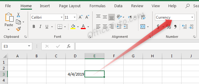
Typing a number into this cell and pressing enter will not just show that number, but will instead format it accordingly.
Before pressing enter, Excel shows the value which was typed: “4”.
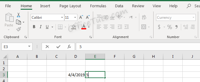
After pressing enter, the value is updated based on the formatting type selected.
Don’t let the format type showed in the illustration at the drop-down list confusing you; it is reflecting the cell below (i.e. E4), since we validated by an Enter.
2- Number format
Cells formatted as numbers behave differently than general formatted cells. By default, when a number is entered, or when a cell is formatted as a number already, the alignment of the information within the cell will be on the right instead of on the left. This makes it easier to read a list of numbers such as the below.
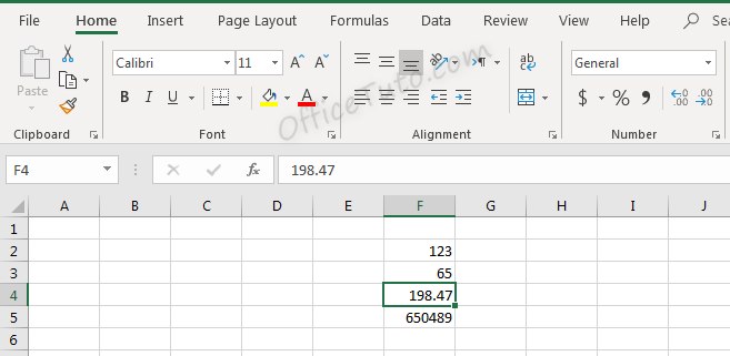
Note in the above screenshot that since we didn’t choose the “Number” format for our cells, they still have a “General” one. They are numbers for Excel (meaning, we can do calculations on them), but they didn’t have yet the number format and its formatting aspects:
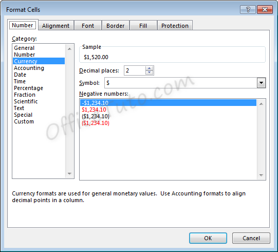
You can set the formatting options for Excel numbers in the “Format Cells” dialog box.
To do that, select the cell or the range of cells you want to set the formatting options for their numbers, and go to the “Home” tab of the ribbon, then in the “Number” group of commands, click on the launcher of the dialog box (the arrow on the right-down side of the group).
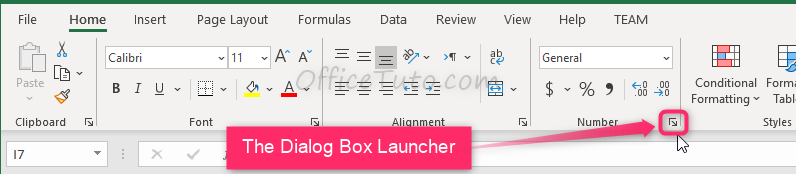
Excel opens the “Format Cells” dialog box in its “Number” tab. Click in the “Category” pane on “Number”.
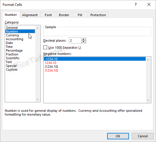
- In this dialog box, you can decide how many decimal places to display by updating options in the “Decimal places” field.
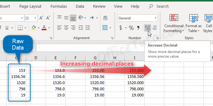
Note that this feature is also available in the “Home” tab of the ribbon where you can go to the “Number” group of commands and click the Increase Decimal ![]() or Decrease Decimal
or Decrease Decimal ![]() buttons.
buttons.
Here is the result of consecutive increasing of decimal places on our example of data (1 decimal; 2 decimals; and 3 decimals):
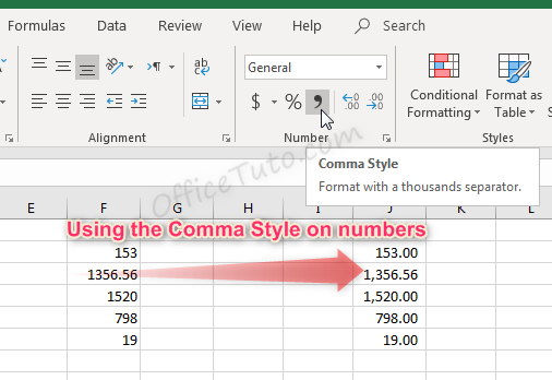
- You can also decide if commas should be shown in the display as a thousand separator, by updating the “Use 1000 Separator (,)” option in the “Format Cells” dialog box.
This feature is also available in the “Home” tab of the ribbon by clicking the “Comma Style” button ![]() in the “Number” group of commands.
in the “Number” group of commands.
Note that using the Comma Style button will automatically set the format to Accounting.
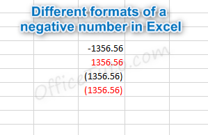
- Another option from the Format Cells dialog box is to decide how negative numbers should display by using the “Negative numbers” field.
There are four options for displaying negative
numbers.
- Display
negative numbers with a negative sign before the number. - Display
negative numbers in red. - Display
negative numbers in parentheses. - Display
negative numbers in red and in parentheses.
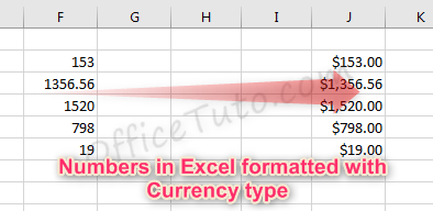
3- Currency format
Cells formatted as currency have a currency symbol such as a dollar sign $ immediately to the left of the number in the cell, and contain two numbers after the decimal by default.
The alignment of numbers in currency formatted cells will be on the right for readability.
Currency formatting options are similar to
number formatting options, apart from the currency symbol display.
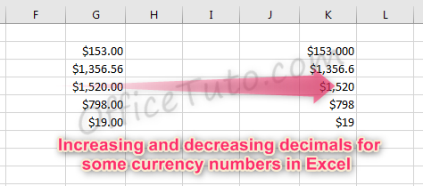
- As with regular number formatting, you can decide, in the “Format Cells” dialog box, how many decimal places to display by updating the field “Decimal places”.
You can also find this feature in the “Home” tab of the ribbon, by going to the “Number” group of commands and clicking the Increase Decimal ![]() or Decrease Decimal
or Decrease Decimal ![]() .
.
- You can also decide what currency symbol should be shown in the display by updating the “Symbol” field in the “Format Cells” dialog box.
- As with regular number formatting, you can also decide how negative numbers should display by updating the “Negative numbers” field in the “Format Cells” dialog box.
There are four
options for displaying negative numbers.
- Display
negative numbers with a negative sign before the number. - Display
negative numbers in red. - Display
negative numbers in parentheses. - Display
negative numbers in red and in parentheses.
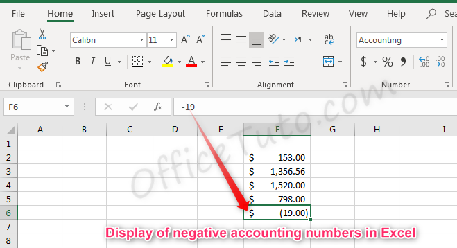
4- Accounting format
Like with the currency format, cells formatted as accounting have a currency symbol such as a dollar sign $; however, this symbol is to the far left of the cell, while the alignment of numbers in the cell is on the right. Accounting numbers contain two numbers after the decimal by default.
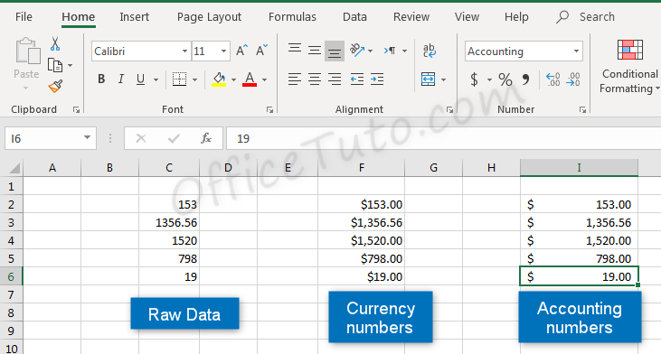
Clicking the “Accounting Number Format” button ![]() in the “Number” group of commands of the “Home” tab, will quickly format a cell or cells as Accounting.
in the “Number” group of commands of the “Home” tab, will quickly format a cell or cells as Accounting.
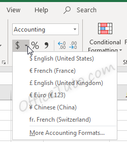
The down arrow to the right of the Accounting Number Format button allows selection between common symbols used for accounting, including English (dollar sign), English (pound), Euro, Chinese, and French symbols.
Accounting formatting options in the “Format Cells” dialog box (“Home” tab of the ribbon, in the “Number” group of commands, click on the launcher of the “Number Format” dialog box), are similar to number and currency formatting options.
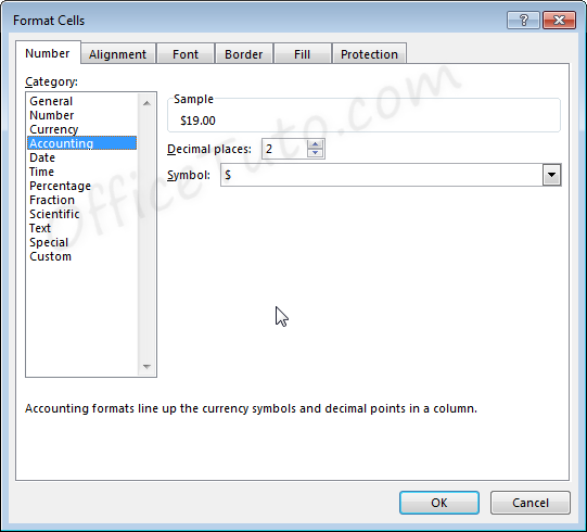
- You can decide how many decimal places to display by updating its option in the “Format Cells” dialog box.
As mentioned before in this tutorial, this feature is also available directly in the “Home” tab of the ribbon by clicking the Increase Decimal ![]() or Decrease Decimal
or Decrease Decimal ![]() buttons in the “Number” group of commands.
buttons in the “Number” group of commands.
- You can also decide in the “Format Cells” dialog box, what currency symbol should be shown in the display by using the “Symbol” drop-down list.
This dropdown gives a much broader list of options than the “Accounting Number Format” option in the “Home” tab of the ribbon.
Note that with the Accounting formatting option, negative numbers display in parentheses by default. There are not options to change this.
5- Date format
There are options for “Short Date” and “Long Date” in the “Number Format” dropdown list of the “Home” tab.
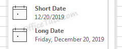
Short date shows the date with slashes separating month, day, and year. The order of the month and day may vary depending on your computer’s location settings.
Long date shows the date with the day of the week, month, day, and year separated by commas.
More options for formatting dates are available in the “Format Cells” dialog box (accessible by clicking in the “Number Format” dropdown list of the “Home” tab and choosing the “More Number Formats” option at the bottom).
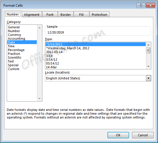
- You can choose from a long list of available date formats.
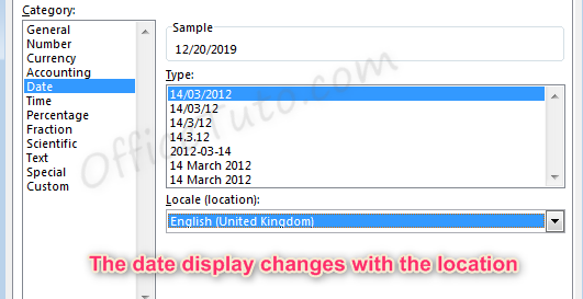
- You can update the location settings used for formatting the date. This will alter the list of format options in the above list and will adjust the display and potentially the order of the elements (day, month, year) within the date.
Note the below example when we switch from English (United States) format to English (United Kingdom) format.
6- Time format
Cells formatted as time display the time of
day. The default time display is based on your computer’s location settings.
Time formatting options are available in the “Format Cells” dialog box (accessible by choosing the “More Number Formats” option at the bottom of the “Number Format” dropdown list in the “Home” tab of the ribbon).
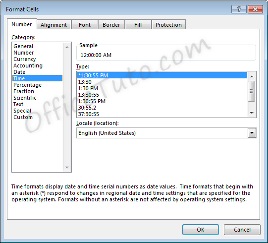
- You can choose from a long list of available time formats.
- You can update the location settings used for formatting the time. This will alter the list of format options in the above list and will adjust the display.
7- Percentage format
Cells formatted as percentage display a percent sign to the right of the number. You can change the format of a cell to a percentage using the “Number Format” dropdown list, or by clicking the “Percent Style” button ![]() . Both options are accessible from the “Home” tab of the ribbon, in the “Number” group of commands.
. Both options are accessible from the “Home” tab of the ribbon, in the “Number” group of commands.
Note that updating a number to a percentage
will expect that the number already contains the decimal. For example:
A cell containing the value 0.08, as a percentage, will show 8%.
A cell containing the value 8, as a percentage, will show 800%.
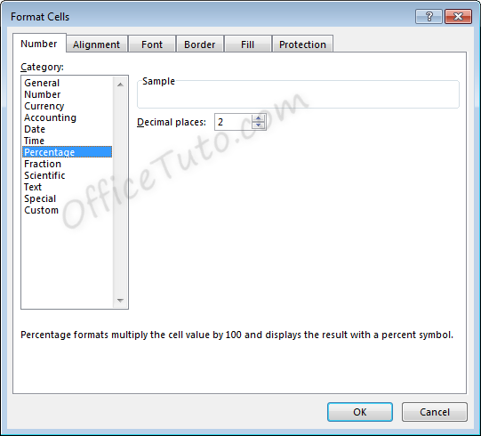
Percentage formatting options are available in the “Format Cells” dialog box, accessible by clicking on “More Number Formats” of the “Number Format” dropdown list in the “Home” tab of the ribbon.
8- Fraction format
Cells formatted as a fraction display with a slash
symbol separating the numerator and denominator.
Fraction formatting options are available in the “Format Cells” dialog box, accessible by clicking in the “Home” tab of the ribbon, on “More Number Formats” of the “Number Format” dropdown list.
- Note that
when selecting the format to use for a fraction, Excel will round to the
nearest fraction where the formatting criteria can be met.
As an example, if the
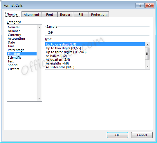
formatting option selected is “Up to one digit”, entering a fraction with two
digits will cause rounding to occur. For example, with the setting of “Up to
one digit”,
If we enter a value of 7/16, the value displayed will be 4/9, as converting to 9ths was the option with only one digit which required the least amount of rounding.
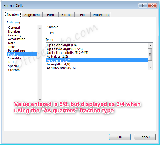
For another example, if the formatting option selected is “As quarters”, entering a fraction that cannot be expressed in quarters (divisible by four) will also cause rounding to occur.
If we enter a value of 5/8, the value displayed will be 3/4. Excel rounded up to 6/8, or 3/4, which was the closest option divisible by four.
- Also note
that for the formatting options with “Up to x digits”, Excel will always round
down to the lowest exact equivalent fraction when possible.
For example, if we enter a value of 2/4 with one of these formatting options active, the value displayed will be 1/2, as this is the mathematical equivalent. This behavior will not take place for formatting options “As…”, since these specifically determine what the denominator should be.
- Fractions listed as more than a whole (meaning the numerator is a higher number than the denominator), such as 7/4 will automatically be adjusted into a whole number and a fraction 13/4, where the fraction follows the formatting rules selected.
9- Scientific format
Scientific format, otherwise known as
Exponential Notation, allows very large and small numbers to be accurately
represented within a cell, even when the size of the cell cannot accommodate
the size of the numbers.
The way exponential notation works is to theoretically place a decimal in a spot that would make the number shorter, then describe where to move that decimal to return to the original number.
Examples with large numbers, where the decimal is moved to the left:
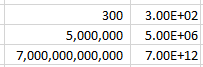
For the number 300 to be expressed in
exponential notation, Excel moves the decimal from after the whole number
300.00 to between the 3 and the 00. This is typed out as E+02 since the decimal
was moved two places to the left. The other examples are similar, where the
decimal was moved 6 and 12 places to the left.
Examples with small numbers, where the decimal is moved to the right:
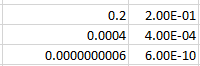
For the number 0.2 to be expressed in
exponential notation, Excel moves the decimal to create a whole number 2. This
is typed out as E-01 since the decimal was moved one place to the right. The
other examples are similar, where the decimal was moved 4 and 10 places to the
right.
Scientific formatting options are listed in the “Format Cells” dialog box, accessible by going to the “Home” tab of the ribbon, and clicking the “More Number Formats” option of the “Number Format” dropdown list.
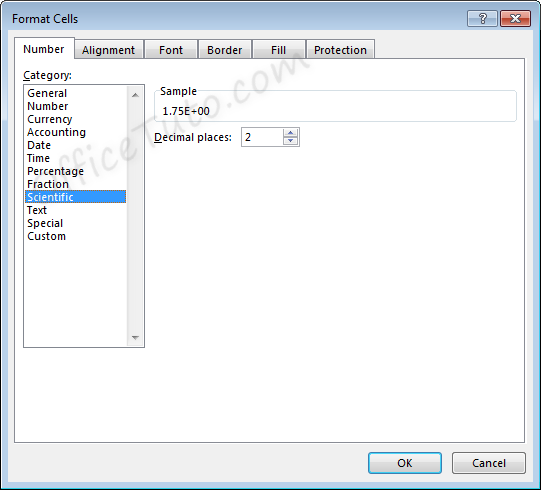
The only option available is to alter the
number of decimal places shown in the number prior to the scientific notation.
For example, for the value 11.43 formatted with the scientific format, if we change the Decimal places from 2 to 1, the display will change as follows.
Two decimals: 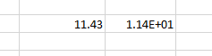
One decimal: 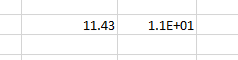
10- Text format
Cells can be formatted as Text through the
“Number Format” dropdown list, in the “Number” group of commands of the “Home”
tab.
Using the Text format in Excel allows values to be entered as they are, without Excel changing them per the above formatting rules.
In general, when entering a text in a cell, you won’t need to set its type to “Text”, as the default format type “General” is sufficient in most cases.
This may be useful when you want to display numbers with leading zeros, want to have spaces before or after numbers or letters, or when you want to display symbols that Excel normally uses for formulas.
Below are examples of some fields formatted as Text.
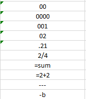
Note that when a number is formatted as Text, Excel will display a symbol showing that there could be a possible error ![]() .
.
Clicking the cell, then clicking the pop-up icon will show what the error may be and offer suggestions for resolution.
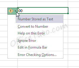
11- Special format
Special format offers four options in the “Format Cells” dialog box, accessible by going to the “Home” tab of the ribbon, and clicking the launcher arrow in the “Number” group of commands.
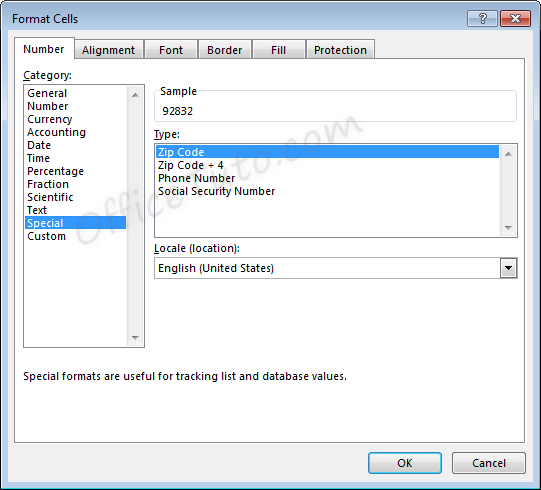
- Zip Code
When less than five numbers are entered in Zip
Code format, leading zeros will be added to bring the total to five numbers.
When more than five numbers are entered in Zip Code format, all numbers will be displayed, even though this does not meet the format criteria.
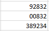
- Zip Code + 4
Zip Code + 4 format automatically creates a
dash symbol – before the last four numbers in the zip code.
When less than nine numbers are entered in Zip
Code + 4 format, leading zeros will be added to bring the total to nine
numbers.
When more than nine numbers are entered in Zip Code + 4 format, extra numbers are displayed prior to the dash symbol –.
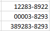
- Phone Number
Phone Number format automatically creates a
dash –
before the last four numbers in the phone number. This format also adds
parentheses ( ) around the area code when an area code is entered.
When less than the expected number of digits
are entered in Phone Number format, only the entered digits will be displayed,
starting from the end of the phone number, as shown on the third and fourth
lines, below.
When more than the expected number of digits
are entered in Phone Number format, extra numbers are displayed within the area
code parentheses.
Note that Phone Number format in Excel does not handle the number 1 before an area code. This entry would be treated like any other extra number.
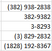
- Social Security Number
Social Security Number format automatically
creates a dash – before the last four numbers in the social security number
and a dash before the last six numbers in the social security number.
When less than nine numbers are entered in
Social Security Number format, leading zeros will be added to bring the total
to nine numbers.
When more than nine numbers are entered in Social Security Number format, extra numbers are displayed prior to the first dash –.
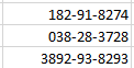
12- Custom format
Custom formats can be used or added through the
“Format Cells” dialog box, accessible from the “Number” group of commands in
the “Home” tab of the ribbon by clicking the “Number Format” launcher arrow.
This can be useful if the above formatting options do not work for your needs. Custom number formats can be created or updated by typing into the “Type” field of the “Format Cells” dialog box.
When creating a new custom format, be sure to use an existing custom format that you are okay with changing.
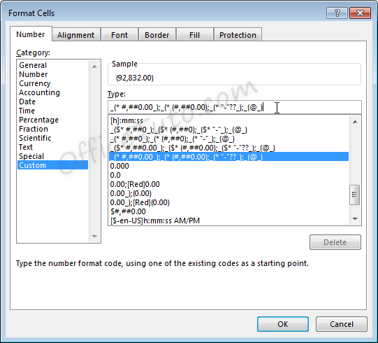
Custom number formats are separated, at
maximum, into four parts separated by semicolons ; .
- Part 1: How
to handle positive number values - Part 2: How
to handle negative number values - Part 3: How
to handle zero number values - Part 4: How
to handle text values
Note that if fewer parts are included in the custom format coding, Excel will determine how best to merge the above options: As an example, if two parts are listed, positive and zero values will be grouped.
Note that Excel may update the formatting of some fields to Custom automatically depending on what actions are taken on the field.
C- Common issues caused by wrong cell format types in Excel
1- Common issues due to wrong cell format types in Excel
The most common problems you may encounter with a wrong cell format type in Excel are of 3 types:
– Getting a wrong value.
– Getting an error.
– Formula displayed as-is and not calculated.
Let’s illustrate these 3 cases with some examples:
- Getting a wrong value
This may occur when you enter a value in an already formatted cell with an inappropriate format type, or when you apply a different format to a cell already containing a value.
The following table details some examples:
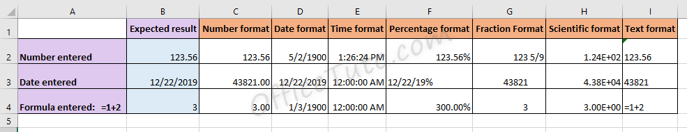
- Getting an error
This occurs when you enter a text preceded with a symbol of a dash, or plus, or equal, as an element of a list.
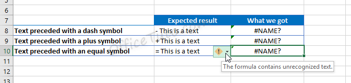
Excel wrongly interprets the text as a formula and show the error “The formula contains unrecognized text”.
- Formula displayed as-is and not calculated
In the following example, we tried to calculate the total of prices from cell B2 to B6 using the Excel SUM function, but Excel doesn’t calculate our formula and just displayed it as-is.
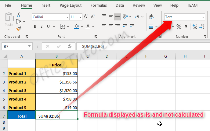
The source of the problem is that the result cell, B7, was previously formatted as text before entering the formula.
2- How to correct wrong cell format type issues in Excel
To correct cell format type issues in Excel, apply the right format in the “Number Format” drop-down list, and sometimes, you’ll also need to re-enter the content of the cell. For cells with formulas displayed as text, choose the “General” format, then double click in the cell and press Enter.

Jeff Golden is an experienced IT specialist and web publisher that has worked in the IT industry since 2010, with a focus on Office applications.
On this website, Jeff shares his insights and expertise on the different Office applications, especially Word and Excel.
In this post, we’re going to learn everything there is to know about Excel Tables!
Yes, I mean everything and there’s a lot.
This post will tell you about all the awesome features Excel Tables have and why you should start using them.
What is an Excel Table?
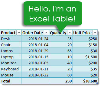
Excel Tables are containers for your data.
Imagine a house without any closets or cupboards to store your things, it would be chaos! Excel tables are like closets and cupboards for your data, they help to contain and organize data in your spreadsheets.
In your house, you might put all your plates into one kitchen cupboard. Similarly, you might put all your customer data into one Excel table.
Tables tell excel that all the data is related. Without a table, the only thing relating the data is proximity to each other.
Ok, so what’s so great about Excel Tables other than being a container to organize data? A lot actually. This post will tell you about all the awesome features tables have and should convince you to start using them.
Video Tutorial
The Parts of a Table
Throughout this post, I’ll be referring to various parts of a table, so it’s probably a good idea that we’re both talking about the same thing.
This is the Column Header Row. It is the first row in a table and contains the column headings that identify each column of data. Column headings must be unique in the table, they cannot be blank and they cannot contain formulas.
This is the Body of the table. The body is where all the data and formulas live.
This is a Row in the table. The body of a table can contain one or more rows and if you try to delete all the rows in a table a single blank row will remain.
This is a Column in the table. A table must contain at least one column.
This is the Total Row of the table. By default, tables don’t include a total row but this feature can be enabled if desired. If it’s enabled, it will be the last row of the table. This row can contain text, formula or remain blank. Each cell in the total row will have a drop down menu that allows selection of various summary formula.
Create a Table from the Ribbon
Creating an Excel Table is really easy. Select any cell inside your data and Excel will guess the range of your data when creating the table. You’ll be able to confirm this range later on. Instead of letting Excel guess the range you can also select the entire range of data in this step.
With the active cell inside your data range, go to the Insert tab in the ribbon and press the Table button found in the Tables section.
The Create Table dialog box will pop up. Excel guesses the range and you can adjust this range if needed using the range selector icon on the right hand side of the Where is the data for your table? input field. You can also adjust this range by manually typing over the range in the input field.
Checking the My table has headers box will tell Excel the first row of data contains the column headers in your table. If this is unchecked Excel will create generic column headers for the table labelled Column 1, Column 2 etc…
Press the Ok button when you’re satisfied with the data range and table headers check box.
Congratulations! You now have an Excel table and your data should look something like the above depending on the default style of your tables.
Contextual Table Tools Design Tab
Whenever you select a cell inside a table, you will notice a new tab appear in the ribbon labelled Table Tools Design. This is a contextual tab and only appears when a table is selected. When the active cell moves outside the table, the tab will disappear again.
This is where all the commands and options related to tables will live. This is where you’ll be able to name your table, find table related tools, enable or disable table elements and change your table’s style.
Create a Table with a Keyboard Shortcut
You can also create a table using a keyboard shortcut. The process is the same as described above but instead of using the Table button in the ribbon you can press Ctrl + T on your keyboard. It’s easy to remember since T is for Table!
There is actually another keyboard shortcut that you can use to create tables, Ctrl + L will also do the same thing. This is a legacy from when tables were called lists (L is for List).
Name a Table
Anytime you create a new table Excel will give it an initial generic name starting with Table1 and increasing sequentially. You should always rename your table with a descriptive and short name.
Not all names are allowed. There are a few rules for a table name.
- Each table must have a unique name within a workbook.
- You can only use letters, numbers and the underscore character in a table name. No spaces or other special characters are allowed.
- A table name must begin with either a letter or an underscore, it can not begin with a number.
- A table name can have a maximum of 255 characters.
Select any cell inside your table and the contextual Table Tools Design tab will appear in the ribbon. Inside this tab you can find the Table Name under the Properties section. Type over the generic name with your new name and press the Enter button when finished to confirm the new name.
Rename a Table
Renaming a table you’ve already named is the same process as naming a table for the first time. If you think about it, when you first name a table you’re actually renaming it from the generic name of Table1 to a new name.
So go back to the Table Tools Design tab and type your new name over the old one in the Table Name and press Enter. Easy, and the name is changed.
Changing your table name this way requires navigating to your table and selecting a cell within it, so it can be tedious if you need to rename a lot of tables across different sheets in your workbook. Instead, you can change any of your table names without going to each table using the Name Manager.
Go to the Formula tab and press the Name Manager button in the Defined Names section. You’ll be able to see all your named objects here. The table objects will have a small table icon to the left of the name. You can filter to show only the table objects using the Filter button in the upper right hand corner and selecting Table Names from the options.
You can then edit any name by selecting the item and pressing the Edit button. You’ll be able to change the name and add some comments to describe the data in your table.
Navigate Tables with the Name Box
You can easily navigate to any table in your workbook using the name box the the left of the formula bar. Click on the small arrow on the right side of the name box and you will see all table names in the workbook listed. Click on any of the tables listed and you will be taken to that table.
Convert a Table Back to a Normal Range
Ok, you changed your mind and don’t want your data inside a table anymore. How do you convert it back into a regular range?
If changing it to a table was the last thing you did, Ctrl + Z to undo your last action is probably the quickest way.
If it wasn’t the last thing you did, then you’re going to need to use the Convert to Range command found in the Table Tools Design tab under the Tools section.
You’ll be prompted to confirm that you really want to convert the table to a normal range. Noooooo, don’t do it, tables are awesome!
If you click on yes, then all the awesome benefits from tables will be gone except for the formatting design. You’ll need to manually clear this from the range if you want to get rid it. You can do this by going to the Home tab then pressing the Clear button found in the Editing section, then selecting Clear Formats.
This can also be done from the right click menu. Right click anywhere in the table and select Table from the menu and then Convert to Range.
Select the Entire Column
If your data is not inside a table then selecting an entire column of the data can be difficult. The usual way would be to select the first cell in the column and then hold Ctrl + Shift then press the Down arrow key. If the column has blank cells, then you might need to press the Down arrow key a few times until you reach the end of the data.
The other option is to select the first cell and then use the scroll bar to scroll to the end of your data then hold the Shift key while you select the last column.
Both options can be tedious if you have a lot of data or there are a lot of blanks cells in the data.
With a table, you can easily select the entire column regardless of blank cells. Hover the mouse cursor over the column heading until it turns into a small arrow pointing down then left click and the entire column will be selected. Left click a second time to include the column heading and any total row in the selection.
Another way to quickly select the entire column is to place the active cell cursor on any cell in the column and press Ctrl + Space. This will select the entire column excluding the column header and total row. Press Ctrl + Space again to include the column headers and total row.
Select the Entire Row
Selecting the entire row is just as easy. Hover the mouse cursor over the left side of the row until it turns into a small arrow pointing left then left click and the entire row will be selected. This works on both the column heading row and total row.
Another way to quickly select the entire row is to place the active cell cursor on any cell in the row and press Shift + Space.
Select the Entire Table
It’s also possible to select the entire table and there are a couple different ways to do this.
You can place the active cell cursor inside the table and press Ctrl + A. This will select the entire body of the table excluding the column headers and total row. Press Ctrl + A again to include the column headers and total row.
Hover the mouse over the top left hand corner of the table until the cursor turns into a small black diagonal right and downward pointing arrow. Left click once to select only the body. Left click a second time to include the header row and total row.
You can also select the table with the mouse. Place the active cell inside the table and then hover the mouse cursor over any edge of the table until it turns into a four way directional arrow then left click. This will also select the column headers and total row.
Select Parts of the Table from the Right Click Menu
You can also select rows, columns or the entire table using the right click menu. Right click anywhere on the row or column you want to select then choose Select and pick from the three options available.
Add a Total Row
You can add a total row which allows you to display summary calculations in the last row of your table.
Adding summary calculations at the bottom of your data can be dangerous as they might end up getting included by accident in a pivot table using the data. This is another advantage of tables, as the total row won’t be included in any pivot tables created with the table.
To enable the total row, go to the Table Tools Design tab and check the Total Row box found in the Table Style Options section.
You can temporarily disable the total row without losing the formulas you added to it. Excel will remember the formulas you had and they will appear when you enable it again.
Each cell in the total row has a drop down menu that allows you to pick various aggregating functions to summarize the column of data above.
You can also enter your own formulas. I’ve entered a SUMPRODUCT formula in the Unit Price total to sum the Quantity x Unit Price to calculate a total sale amount. Formulas don’t have to return a number, they can also be text results.
Constant numerical or text values are also allowed anywhere in the total row. In fact the leftmost column will usually contain the text Total by default.
Add a Total Row with a Right Click
You can also add the total row with a right click. Right click anywhere on the table and the choose Table and Total Row from the menu.
Add a Total Row with a Keyboard Shortcut
Another way to quickly add the total row is to place the active cell cursor inside your table and use the Ctrl + Shift + T keyboard shortcut.
Disable the Column Header Row
The column header row is enabled by default, but you can disable it. This doesn’t delete the column headers, it’s essentially like hiding them as you will still reference columns based on the column header name.
Go to the Table Tools Design tab and uncheck the Total Row box found in the Table Style Options section.
Add Bold Format to the First or Last Columns
You can enable a bold formatting on either your first or last column to highlight it and draw attention to them over other columns.
Go to the Table Tools Design tab and check either of the First Column or Last Column boxes (or both) found in the Table Style Options section.
Add Banded Rows or Columns
Banded rows are already enabled by default, but you can turn them off if you want. Banded columns are disabled by default, so you need to enable them if you want them.
To enable or disable either, go to the Table Tools Design tab and check or uncheck the Banded Rows or Banded Columns boxes found in the Table Style Options section.
I generally find banded rows are the most useful and if you enable banded columns at the same time, the table starts to look a little messy. I recommend one or the other and not both at the same time.
- Table with no banded rows or columns.
- Table with banded rows only.
- Table with banded columns only.
- Table with both banded rows and columns.
Table Filters
By default, the table filters option is enabled. You can disable them from the Table Tools Design tab by unchecking the Filter Button box found in the Table Style Options section.
You can also toggle the filters on or off from the active table by using the regular filter keyboard shortcut of Ctrl + Shift + L.
If you left click on any of the filters, it will bring up the familiar filter menu where you can sort your table and apply various filters depending on the type of data in the column.
The great thing about table filters is you can have them on multiple tables in the same sheet simultaneously. You will need to be careful though as filtered items in one table will affect the other tables if they share common rows. You can only have one set of filters at a time in a sheet of data without tables.
Total Row with Filters Applied
When you select a summary function from the drop down menu in the total row, Excel will create the corresponding SUBTOTAL formula. This SUBTOTAL formula ignores hidden and filtered items. So when you filter your table these summaries will update accordingly to exclude the filtered values.
Note that the SUMPRODUCT formula in the Unit Price column still includes all the filtered values while the SUBTOTAL sum formula in the Quantity column does not.
Column Headers Remain Visible When Scrolling
If you scroll down while the active cell is in a table, its column headers will remain visible along with the filter buttons. The table’s column headings will get promoted into the sheet’s column headings where we would normally see the alphabetic column name.
This is extremely handy when dealing with long tables as you won’t need to scroll back up to the top to see the column name or use the filters.
Automatically Include New Rows and Columns
If you type or copy and paste new data into the cells directly below a table, they will automatically be absorbed into the table.
The same thing happens when you type or copy and paste into the cells directly to the right of a table.
Automatically Fill Formulas Down the Entire Column
When you enter a formula inside a table it will automatically fill the formula down the entire column.
Even when a formula has already been entered and you add new data to the row directly below the table any existing formulas will automatically fill.
Editing an existing formula in any of the cells will also update the formula in the entire column. You’ll never forget to copy and paste down a formula again!
Turn Off the Auto Include and Auto Fill Settings
You can turn off the feature that automatically adds new rows or columns and fills down formulas.
Go to the File tab and select Options. Choose Proofing then press the AutoCorrect Options button. Navigate to the AutoFormat As You Type tab in the AutoCorrect dialog box.
Unchecking the Include new rows and columns in table option allows you to type directly underneath or to the right of a table without it absorbing the cells.
Unchecking the Fill formulas in tables to create calculated columns option means the formulas in a table will no longer automatically fill down the column.
Resize with the Handle
Every table comes with a Size Handle found in the bottom rightmost cell of the table.
When you hover the mouse over the handle, the cursor will turn into a double-sided diagonally slanting arrow and you can then click and drag to resize the table. You can either expand or contract the size. Data will be absorbed into the table or removed from it accordingly.
Resize with the Ribbon
You can also resize the table from the ribbon. Go to the Table Tools Design tab and press the Resize Table command in the Properties section.
The Resize Table dialog box will pop up and you’ll be able to select a new range for your table. Use the range selector icon to select a new range. You can select either a larger or smaller range, but The table headers will need to remain in the same row and the new table range must overlap the old table range.
Add a New Row with the Tab Key
You can add a new blank row to a table with the Tab key. Place the active cell cursor inside the table on the cell containing the sizing handle and press the Tab key.
The tab key act like a carriage return and the active cell is taken to the rightmost cell on a new line that’s added directly below.
This is a handy shortcut to know because when the total row is enabled, it’s not possible to add a new row by typing or copying and pasting data directly below the table.
Insert Rows or Columns
You can insert extra rows or columns into a table with a right click. Select a range in the table and right click then choose Insert from the menu. You can then either choose to insert Table Columns to the Left or Table Rows Above.
Table Columns to the Left will insert the number of columns selected to the left of the selection and the number of rows in the selection is ignored.
Table Rows Above will insert the number of rows selected just above the selection and the number of columns in the selection is ignored.
Delete Rows or Columns
Deleting rows or columns has a similar story to inserting them. Select a range in the table and right click then choose Delete from the menu. You can then either choose to delete Table Columns or Table Rows.
Formats in a Table Automatically Apply to New Rows
When you add new data to your table, you don’t need to worry about applying formatting to match the rest of the data above. Formatting will automatically fill down from above if the formatting has been applied to the entire column.
I’m not just talking about the table style formats. Other formatting like dates, numbers, fonts, alignments, borders, conditional formatting, cell colours etc. will all automatically fill down if they’ve been applied to the whole column.
If you’ve formatted all your numbers as a currency in a column and you add new data, it too will get the currency format applied to it.
You never need to worry about inconsistent formatting in your data.
Add a Slicer
You can add a slicer (or several) to a table for an easy to use filter and visual way to see what items the table is filtered on.
Go to the Table Tools Design tab and press the Insert Slicer button found in the Tools section.
Change the Style
Changing the styling of a table is quick and easy. Go to the Table Tools Design select a new style from the selection found in the Table Styles section. If you left click the small downward arrow on the right hand side of the styles palette, it will expand to show all available options.
These table styles apply to the whole table and will also apply to any new rows or columns added later on.
There are many options to choose from including light, medium and dark themes. As you hover over the various selections, you’ll be able to see a live preview in the worksheet. The style won’t actually change until you click on one though.
You can even create your own New Table Style.
Set a Default Table Style
You can set any of the styles available as the default so that when you create a new table you don’t need to change the style. Right click on the style you want to set as the default and then choose Set As Default from the menu.
Unfortunately, this is a workbook level setting and will only affect the current workbook. You will need to set the default for each workbook you create if you don’t want the application default option.
Only Print the Selected Table
When you place the active cell cursor inside a table and then try to print, there is an option to only print the selected table. Go to the Print menu screen by either going to the File tab and selecting Print or using the Ctrl + P keyboard shortcut, then select Print Selected Table in the settings.
This will remove any items from the print area that are not in the table.
Structured Referencing
Tables come with a useful feature called structured referencing which helps to make range references more readable. Ranges within a table can be referred to using a combination of the table name and column headings.
Instead of seeing a formula like this =SUM(D3:D9) you might see something like this =SUM(Sales[Quantity]) which is much easier to understand the meaning of.
This is why naming your table with a short descriptive name and column headings is important as it will improve the readability of the structured references!
When you reference specific parts of a table, Excel will create the reference for you so you don’t need to memorize the reference structure but it will help to understand it a bit.
Structured references can contain up to three parts.
- This is the table name. When referencing a range from inside the table this part of the reference is not required.
- These are range identifiers and identify certain parts of the reference for a table like the headers or total row.
- These are the column names and will either be a single column or a range of columns separated by a full colon.
Example of structured References for a Row
=Sales[@[Unit Price]]will reference a single cell in the body.=Sales[@[Product]:[Unit Price]]will reference part of the row from the Product column to the Unit Price column including all columns in between.=Sales[@]will reference the full row.
Example of Structured References for Columns
=Sales[Unit Price]will reference a single column and only include the body.=Sales[[#Headers],[#Data],[Unit Price]]will reference a single column and include the column header and body.=Sales[[#Data],[#Totals],[Unit Price]]will reference a single column and include the body and total row.=Sales[[#All],[Unit Price]]will reference a single column and include the column header, body and total row.
Example of Structured References for the Total Row
=Sales[#Totals]will reference the entire total row.=Sales[[#Totals],[Unit Price]]will reference a cell in the total row.=Sales[[#Totals],[Product]:[Unit Price]]will reference part of the total row from the Product column to the Unit Price column including all columns in between.
Example of Structured References for the Column Header Row
=Sales[#Headers]will reference the entire column header row.=Sales[[#Headers],[Order Date]]will reference a cell in the column header row.=Sales[[#Headers],[Product]:[Unit Price]]will reference part of the column header row from the Product column to the Unit Price column including all columns in between.
Example of Structured References for the Table Body
=Saleswill reference the entire body.=Sales[[#Headers],[#Data]]will reference the entire column header row and body.=Sales[[#Data],[#Totals]]will reference the entire body and total row.=Sales[#All]will reference the entire column header row, body and total row.
Using Intellisense
One of the great things about a table is the structured references will appear in Intellisense menus when writing formulas. This means you can easily write a formula using the structured references without remembering all the fields in your table.
After typing the first letter of the table name, the IntelliSense menu will show the table name among all the other objects starting with that letter. You can use the arrow keys to navigate to it and then press the Tab key to autocomplete the table name in your formula.
If you want to reference a part of the table, you can then type a [ to bring up all the available items in the table. Again, you can navigate with the arrow keys and then use the Tab key to autocomplete the field name. Then you can close the item with a ].
Turn Off Structured Referencing
If you’re not a fan of being forced to use the structured referencing system, then you can turn it off. Any formulas that have been entered using the structured referencing will remain and they will still work the same. You’ll also still be able to use structured references, Excel just won’t automatically create them for you.
To turn it off, go to the File tab and then select Options. Choose Formulas on the side pane and then uncheck the Use table names in formulas box and press the Ok button.
Summarize with a PivotTable
You can create a pivot table from your table in Table Tools Design tab, press the Summarize with PivotTable button found in the Tools section. This will bring up the Create PivotTable window and you can create a pivot table as usual.
This is the same as creating a pivot table from the Insert tab and doesn’t give any extra options specific to tables.
Remove Duplicates from a Table
You can create remove duplicate rows of data from your table in Table Tools Design tab, press the Remove Duplicates button found in the Tools section. This will bring up the Remove Duplicates window and delete duplicate values for one or more columns in the table.
This is the same as removing duplicates from the Data tab and doesn’t give any extra options specific to tables.
About the Author
John is a Microsoft MVP and qualified actuary with over 15 years of experience. He has worked in a variety of industries, including insurance, ad tech, and most recently Power Platform consulting. He is a keen problem solver and has a passion for using technology to make businesses more efficient.